複雜網路中具縮影性質之階層: 分析及應用

國立交通大學

資訊工程系

博士論文

複雜網路中具縮影性質之階層:

分析及應用

The Abstraction Hierarchy in Complex Networks:

Analyses and Applications

博士生: 鄭家胤

指導教授: 孫春在 教授

國立交通大學

資訊工程系

博士論文

複雜網路中具縮影性質之階層:

分析及應用

The Abstraction Hierarchy in Complex Networks:

Analyses and Applications

博士生: 鄭家胤

指導教授: 孫春在 教授

複雜網路中具縮影性質之階層:

分析及應用

The Abstraction Hierarchy in Complex Networks:

Analyses and Applications

研究生 ：鄭家胤 Student：Chia-Ying Cheng

指導教授：孫春在 Advisor：Chuen-Tsai Sun

國立交通大學

資訊工程系

博士論文

Department of Computer Science College of Computer Science National Chiao Tung University

for the Degree of Doctor of Philosophy

in

Computer Science

July 2009

Hsinchu, Taiwan, Republic of China

i

Abstract (in Chinese)

以複雜網路的型態來呈現複雜系統中的互動關係是一種方便且行之有年的研究 方法，包括在生物學、生態學、社會學等等的領域上，除了讓研究者有不同於以 往該領域傳統議題的新觀點外，許多新的方法也因此被提出來以解決在各種不同 複雜系統上的問題。其中，最重要也最具挑戰性的一個問題就是，如何將複雜網 路做分群(在社會學領域被稱之為共同體(community)或是群組(group)，在生物學 上被稱為基塊(motif)或是模組(module))。如何(1)找出模組，(2)階層性的組織， 及(3)這兩者對應到真實世界的關係，一直是研究者的焦點所在。儘管已經有一 些成功的研究，但是至今仍沒有一個標準的衡量方法可以來找出模組或是階層性 組織。以階層式組織來說，大多數的研究專注於其模組在不同階層上垂直面向的 關係之探討-其可用來表示"包含(inclusion)"，"因果(causality)"和"調控(regulation)" 關係;但往往忽略了其在同一階層上水平面向的關係之研究-其可用來提供給研 究者在某一階層上的網路的縮影(abstraction)或是骨架(backbone)。在本論文研究 中，我提出了一雙向式尋找模組及建構階層組織的方法，其同時考慮了各個模組 間垂直和水平的關係來建構出該複雜系統的金字塔階層(pyramid hierarchies)， 此方法除了被人工網路驗證外，也被應用在生物及社會網路上，其結果顯示該方 法在擷取複雜系統之資訊上卓越的效能。

ii

Abstract (in English)

The use of nodes and links to assemble networks is convenient for representing

interactions in complex systems. This benefits researchers in biology, ecology,

sociology and other biological and social sciences. In addition to supporting

alternative views of complex domains, network research is also supporting new

methods for solving problems in a range of domains. One particularly important and

challenging problem is partitioning networks into clusters (called communities or

groups in social science research and motifs or modules in biology). Research in these

areas has focused on identifying modules and hierarchical organizations that

correspond to real-world meanings (e.g., biological functions or economic and

political constraints). Despite a number of successful examples, no uniform measure

of modularity or standard hierarchical structure exists. Most current descriptions of

hierarchical organizations are limited to vertical relationships between modules at

different hierarchical levels, thus overlooking horizontal relationships that express

associations among modules at the same level. Vertical relationships can be used to

represent inclusion hierarchies and to describe causality/regulation. Horizontal

relationships complement these by providing abstractions of original networks of

iii

In this dissertation I describe a proposal for a two-way simultaneous module-finding

and hierarchy-building strategy. I take both vertical and horizontal relationships

between modules into consideration when building pyramid hierarchies in which each

layer represents an abstraction of lower-level networks. This dissertation also contains

descriptions of tests for this proposed approach, using networks consisting of

anywhere from tens to hundreds of nodes and links, and in domains that include

artificial random networks, social networks, and biological networks. The results

iv

Acknowledgements

I would like to express my deep gratitude to my advisor, Professor Chuen-Tsai Sun,

for teaching me how to define a problem, how to determine its essential components,

and how to identify relationships among those components. I am especially grateful

for the way he modeled the right attitude for students to take when addressing new

topics. That is a skill I will use both in my research and in everyday life.

I also thank my co-advisor, Professor Yuh-Jyh Hu, for his strong support during the

last two years of my Ph.D. research and writing. As a mentor he discussed in great

detail new ideas and ways to implement them. As a friend he shared his life and work

values with me, which helped me stay centered during the entire process.

For all others who were patient with me as I completed this project, I extend my

thanks for your support and patience.

Finally, I give thanks to my Lord Jesus Christ: "And we know that all things work

together for good to those who love God, to those who are called according to His

purpose" (Romans 8:28).

v

Contents

ABSTRACT (IN CHINESE) ... I

ABSTRACT (IN ENGLISH) ... II

ACKNOWLEDGEMENTS ... IV

CONTENTS ... V

LIST OF TABLES ... IX

LIST OF FIGURES ... XI

CHAPTER 1 INTRODUCTION ... 1

1.1 COMPLEX NETWORK TOPOLOGY ... 3

1.1.1 Randomness ... 4

1.1.2 Small-world property ... 5

1.1.3 Scale-free distributions ... 7

1.2 COMPLEX NETWORK STRUCTURE ... 8

1.2.1 Motifs ... 8

1.2.2 Communities ... 11

1.2.3 Hierarchical modularity ... 11

vi

1.3.1 Cellular automata ... 13

1.3.2 Preferential attachment ... 14

CHAPTER 2 STATIC NETWORKS AND DYNAMIC PROCESS CHARACTERIZATION AND ANALYSIS ... 16

2.1 NETWORK MOTIF DETECTION ... 18

2.1.1 General: Bridge and Brick Network Motif-Detecting Algorithm ... 21

2.1.2 Specific: Bridge and Brick Network Motif-Detecting Algorithm ... 26

2.2 SOCIAL NETWORK SIMULATION ... 27

2.3 EPIDEMIC DYNAMICS ANALYSIS ... 29

2.4 ABSTRACTION HIERARCHY ... 33

2.4.1 Proximity Measure ... 34

2.4.2 Network Abstraction ... 43

CHAPTER 3 NETWORK MOTIF EXPERIMENTS ... 45

3.1 GENERAL:BRIDGE AND BRICK NETWORK MOTIF-DETECTING ALGORITHMS ... 45

3.1.1 Validation ... 49

3.1.2 Experiments ... 52

vii

3.2 SPECIFIC:BRIDGE AND BRICK NETWORK MOTIF-DETECTING ALGORITHMS ... 63

3.2.1 Validation ... 63

3.2.2 Experiments ... 67

3.2.3 Conclusion ... 76

CHAPTER 4 SOCIAL NETWORK SIMULATION EXPERIMENTS ... 77

4.1 FRIENDSHIP EVOLUTION AND THE THREE-RULE MODEL ... 77

4.1.1 Friendship Selection Methods ... 79

4.1.2 Friendship Update Equation ... 80

4.1.3 Fitting a Normal Distribution ... 81

4.2 EXPERIMENT ... 83

4.2.1 Effects of Leaving and Arriving ... 85

4.2.2 Effects of Breakup Threshold ... 88

4.2.3 Effects of Resources ... 89

4.2.4 Effects of Initial Friendship ... 90

4.2.5 Distribution of Co-Directors... 92

4.2.6 Sampling ... 94

viii

CHAPTER 5 EPIDEMIC DYNAMICS EXPERIMENTS ... 97

5.1 EPIDEMIC DYNAMICS IN COMPLEX NETWORKS ... 98

5.2 EXPERIMENTS ... 102

5.3 CONCLUSION ... 111

CHAPTER 6 ABSTRACTION HIERARCHY EXPERIMENTS ... 112

6.1 BACKGROUND ... 113

6.2 VALIDATION ... 118

6.3 EXPERIMENTS ... 121

6.3.1 Club network analysis... 122

6.3.2 Football network analysis ... 125

6.3.3 PPI network analysis ... 127

6.3.4 Metabolic network analysis ... 134

CHAPTER 7 CONCLUSION ... 140

ix

List of Tables

TABLE.1.AN UPDATE RULE FOR A ONE-DIMENSIONAL, TWO-STATE CELLULAR AUTOMATON. ... 14

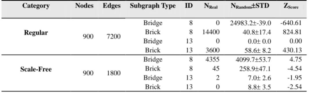
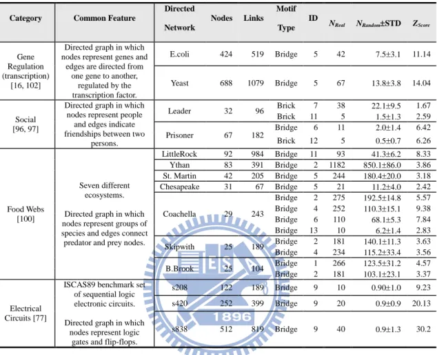
TABLE 2.BRIDGE AND BRICK SUBGRAPH FREQUENCIES IN FOUR COMPLEX NETWORK CATEGORIES (FOR VALIDATION PURPOSES). ... 51

TABLE 3.BRICK AND BRIDGE MOTIFS IN FOURTEEN REAL WORLD NETWORKS, INCLUDING EDGE AND NODE DEFINITIONS, NETWORK SIZES, AND REFERENCES. ... 60

TABLE 4.DESCRIPTIONS OF FIVE GENE REGULATION NETWORKS: EDGE AND NODE DEFINITIONS, NETWORK SIZES, AND REFERENCES. ... 70

TABLE 5.BRICK AND BRIDGE MOTIFS IN FIVE GENE REGULATION NETWORKS... 72

TABLE 6.TERMS AND ABBREVIATIONS FOR INITIALIZED PARAMETERS ... 84

TABLE 7.TERMS AND ABBREVIATIONS FOR STATISTICS ... 85

TABLE 8.EFFECTIVE DIRECTIONS OF THE PARAMETERS ON <K>,C,L ... 92

TABLE 9.CORRELATIONS BETWEEN <K>,C,L FROM EXPERIMENTS ... 92

TABLE 10.SUMMARY OF BIOLOGICAL SIGNIFICANCE OF MODULES BASED ON GO BIOLOGICAL PROCESS ANNOTATIONS ... 131

TABLE 11.SUMMARY OF WITHIN-MODULE CONSISTENCY OF METABOLIC PATHWAY CLASSIFICATION BASED ON KEGG. ... 137

xi

List of Figures

FIG.1.A PYRAMID OF THE COMPLEX NETWORK WITH VERTICAL AND HORIZONTAL RELATIONSHIPS. ... 3

FIG.2.THE COMPARISON BETWEEN THE RANDOM NETWORK AND THE SCALE-FREE NETWORK. ... 8

FIG.3.13 POSSIBLE OF TRIAD MOTIFS DEFINED BY ALON. ... 9

FIG.4.COMMUNITIES CAN BE DEFINED AS GROUPS OF NODES SUCH THAT THERE IS A HIGHER DENSITY OF EDGES WITHIN GROUPS THAN BETWEEN THEM. ... 11

FIG.5.THE HIERARCHICAL NETWORK AND ITS DEGREE DISTRIBUTION. ... 13

FIG.6.NETWORK MOTIFS EXAMPLE. ... 20

FIG.7.LINK-WEIGHTED VALUE CALCULATING EXAMPLE.THE LINK-WEIGHTED VALUE WEIGHT (A, B) OF EDGE (A, B) IS 0 WHILE WEIGHT (B, C) ... 21

FIG.8. THE SMALL-WORLD MODEL.BLACK SIGNIFIES STRONG LINKS AND RED WEAK LINKS. ... 27

FIG.9.THREE-RULE MODEL FLOW DIAGRAM. ... 29

FIG.10FLOWCHART FOR A SIS EPIDEMIOLOGICAL SIMULATION MODEL. ... 33

FIG 11.FOUR SIMPLE NETWORKS TO ILLUSTRATE PROXIMITY MEASURES. ... 39

FIG 12. A SIMPLE UNDIRECTED WEIGHTED NETWORK. ... 41

FIG.13.PERCENTAGES OF BRIDGE AND BRICK MOTIFS IN SMALL-WORLD NETWORKS ACCORDING TO DIFFERENT REWIRING RATIOS. ... 52

xii

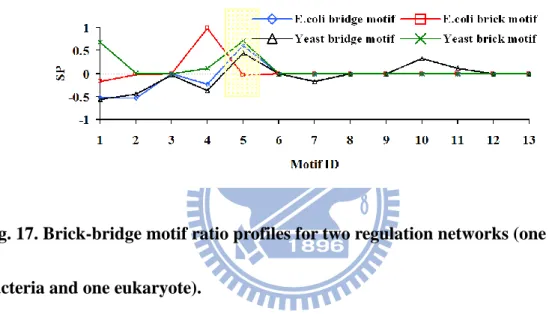
FIG.15.BRIDGE MOTIF RATIO PROFILES FOR TWO SOCIAL NETWORKS. ... 56 FIG.16.BRICK MOTIF RATIO PROFILES FOR TWO SOCIAL NETWORKS. ... 56 FIG.17.BRICK-BRIDGE MOTIF RATIO PROFILES FOR TWO REGULATION NETWORKS (ONE BACTERIA AND

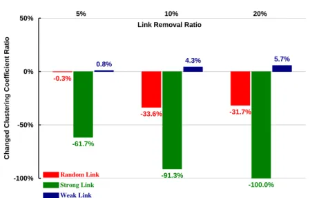
ONE EUKARYOTE). ... 57 FIG.18.BRIDGE MOTIF RATIO PROFILES FOR SEVEN FOOD WEBS... 58 FIG.19. RELATIONSHIPS BETWEEN CLUSTERING COEFFICIENTS AND DIFFERENT REMOVAL RATIOS FOR

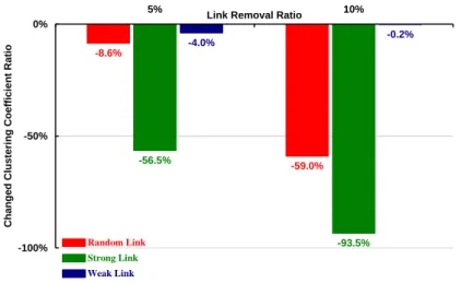
THREE E. COLI LINK TYPES.RED, RANDOM; GREEN, STRONG; BLUE, WEAK. ... 65 FIG.20. RELATIONSHIPS BETWEEN CLUSTERING COEFFICIENTS AND DIFFERENT REMOVAL RATIOS FOR

THREE S. CEREVISIAE (YEAST) LINK TYPES.RED, RANDOM; GREEN, STRONG; BLUE, WEAK. ... 66 FIG.21. COMPARISON OF ORIGINAL (BLUE CURVE) AND ALTERED (RED CURVE) BRICK MOTIF RATIO

PROFILES FOR E. COLI AFTER RANDOMLY REMOVING 40% OF ITS LINKS.ALTERED RESULTS

REPRESENT AVERAGE VALUES FOR 30 RUNS. ... 66 FIG.22.COMPARISON BETWEEN ORIGINAL BRICK MOTIF RATIO PROFILES AND ALTERED BRICK MOTIF

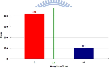
RATIO PROFILES FOR S. CEREVISIAE (YEAST) AFTER RANDOMLY REMOVING 40% OF ITS LINKS. ... 67 FIG.23.DISTRIBUTION OF LINK WEIGHTS IN E.COLI.AVERAGE MEAN AND STANDARD DEVIATION OF LINK

WEIGHTS FOR RANDOMIZED NETWORKS WERE CALCULATED AS 0.900.04. ... 67 FIG.24. COMPARISONS OF TRIAD SIGNIFICANCE PROFILES (TSPS) FOR OUR BRIDGE AND BRICK MOTIFS

xiii

FIG.25. COMPARISONS OF TRIAD SIGNIFICANCE PROFILES (TSPS) FOR OUR BRIDGE AND BRICK MOTIFS

AND MILO ET AL.‘S [7],[28]S. CEREVISIAE (YEAST) MOTIFS. ... 75

FIG.26. BRICK MOTIF RATIO PROFILES FOR TWO GENE REGULATION NETWORKS:E. COLI AND S. CEREVISIAE (YEAST). ... 75

FIG.27. BRIDGE MOTIF RATIO PROFILES FOR THREE GENE REGULATION NETWORKS:C. ELEGANS, SEA URCHIN, AND DROSOPHILA. ... 75

FIG.28.BETA14 PDF CURVES AT DIFFERENT AVERAGES OF 0.1,0.5, AND 0.9. ... 83

FIG.29.COMPARISON OF BETA AND NORMAL DISTRIBUTIONS. ... 83

FIG.30.EXAMPLE OF A STATISTICALLY STATIONARY STATE USING THE PROPOSED MODEL. ... 85

FIG.31.<K>,C AND L VARYING IN BREAKUP THRESHOLD Θ WITH DIFFERENT LEAVING AND ARRIVING PROBABILITY P. ... 87

FIG.32.<K>,C AND L VARYING IN FRIEND-REMEMBERING Q VALUE WITH DIFFERENT DISTRIBUTIONS OF FRIEND-MAKING RESOURCES. ... 88

FIG.33.<K>,C AND L VARYING IN FRIEND-REMEMBERING Q VALUE WITH DIFFERENT DISTRIBUTIONS OF INITIAL FRIENDSHIP F0. ... 89

FIG.34.TWO-RULE MODEL DEGREE DISTRIBUTION P(K). ... 90

FIG.35.<K>,C AND L VARYING IN LEAVING AND ARRIVING PROBABILITY P. ... 92

xiv

FIG.37PREVALENCE Ρ IN STEADY STATE AS A FUNCTION OF EFFECTIVE SPREADING RATE Λ. ... 101 FIG.38.RELATIONSHIP BETWEEN EFFECTIVE SPREADING RATE AND STEADY DENSITY OF THE SIS

EPIDEMIOLOGICAL MODEL ON THREE TYPES OF COMPLEX NETWORK PLATFORMS. ... 104 FIG.39.HOW THE AMOUNT OF AN INDIVIDUAL‘S ECONOMIC RESOURCES AFFECT STEADY DENSITY CURVES.

... 106

FIG.40.RELATIONSHIP BETWEEN RATIO OF TRANSMISSION COSTS TO AN INDIVIDUAL‘S ECONOMIC RESOURCES AND CRITICAL THRESHOLD... 106 FIG.41.HOW DIFFERENT DISTRIBUTION TYPES OF INDIVIDUAL ECONOMIC RESOURCES (DELTA, UNIFORM,

NORMAL, POWER-LAW) AFFECT STEADY DENSITY CURVES AND CRITICAL THRESHOLDS OF

INFECTIOUS DISEASE DIFFUSION IN A SCALE-FREE NETWORK. ... 108 FIG.42.A UNIFORM (N =5, R =2) AND NORMAL DISTRIBUTION (STANDARD DEVIATION =2) OF

INDIVIDUAL ECONOMIC RESOURCES WITH AVERAGE VALUE <R> OF 16. ... 109 FIG.43.INDIVIDUAL ECONOMIC RESOURCES IN A POWER-LAW DISTRIBUTION. ... 109 FIG.44.HOW DIFFERENT TYPES OF INDIVIDUAL ECONOMIC RESOURCE DISTRIBUTIONS (DELTA, UNIFORM,

NORMAL, AND POWER-LAW) AFFECT STEADY DENSITY CURVES AND CRITICAL THRESHOLDS OF INFECTIOUS DISEASE DIFFUSION IN A SCALE-FREE NETWORK. ... 110 FIG.45.A UNIFORM (N =5, R =3) AND NORMAL DISTRIBUTION (STANDARD DEVIATION =3) OF

xv

FIG.46.INDIVIDUAL ECONOMIC RESOURCES IN A POWER-LAW DISTRIBUTION. ... 111

FIG 47.EXAMPLE OF A DENDROGRAM FROM CONVENTIONAL HIERARCHICAL CLUSTERING. ... 118

FIG 48.VALIDATION OF TWO-WAY MODULE-FINDING-HIERARCHY-BUILDING STRATEGY. ... 120

FIG 49.ABSTRACT NETWORK CORRESPONDING TO HIERARCHICAL LEVEL THREE AND TWO. ... 121

FIG.50.CLUSTERING RESULTS OF ZACHARY‘S KARATE CLUB NETWORK. ... 124

FIG.51.THE ANALYSIS OF THE FOOTBALL NETWORK ... 127

FIG.52THE P-VALUE OF THE CORRESPONDING NODES AT DIFFERENT LEVELS. ... 132

FIG.53.THE MST OF PPI AT LEVEL FOUR AND FIVE, AND HAVE BLUE AND RED COLORS, RESPECTIVELY. ... 133

FIG.54.THE MAPPING BETWEEN THE MODULES WE FOUND AND THE REAL GO ID. ... 134

FIG.55.THE PYRAMID OF ABSTRACTION DISCLOSED FROM A METABOLIC NETWORK. ... 138

FIG.56.EXAMPLE OF THE VERTICAL RELATIONSHIPS IN AN ABSTRACTION PYRAMID DISCLOSED FROM A METABOLIC NETWORK. ... 138

FIG.57.EXAMPLE OF THE HORIZONTAL RELATIONSHIP AT THE THIRD LEVEL OF AN ABSTRACTION PYRAMID. ... 139

1

Chapter 1 Introduction

Complex networks consist of sets of items called vertices or nodes and connections

between them called edges. There are many examples of systems in the form of

networks (also called ―graphs‖ in mathematics): the World Wide Web, the Internet, social networks (acquaintances or other connections), distribution networks (e.g.,

blood vessels, postal delivery routes), organizations and business relations, neural

networks, metabolic networks, food webs, and research paper citations, among many

others.

The network concept is proving to be a very useful tool for studying complex systems

[1-3]. While no general theory of complexity exists [2, 4, 5], there is a growing

collection of related theories, paradigms, and tools, many of them associated with

physics and mathematics [5, 6]. They support explanations of complex phenomena

such as collective behavior observed in ferromagnetic phase transitions, herding

behavior, disease epidemics, and opinion formation—all examples of local

interactions that create global order [5, 7]. We also know that even very simple

systems such as discrete logistic growth models (logistic maps) can display rich and

2

systems manage to operate near criticality in the absence of fine-tuning [5, 8]. Fractal

geometry helps explain how and why certain forms and structures in nature arise—for

instance, vascular systems. As a new tool for studying complex phenomena, network

theory uses a mix of statistical mechanics, graph theory, and dynamical systems

theory [9-11].

The majority of network-related problems can be placed in one of two categories: for

static networks, relationships between network structure and function, and for

dynamic networks, global rules tied to network evolution [12-15]. In the following

3

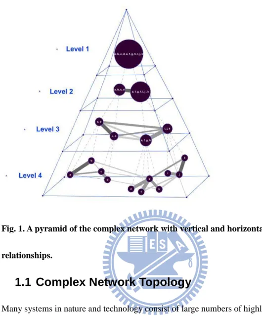
Fig. 1. A pyramid of the complex network with vertical and horizontal relationships.

1.1 Complex Network Topology

Many systems in nature and technology consist of large numbers of highly

interconnected dynamical units [2, 16]. Examples include coupled biological and

chemical systems, neural networks, social interaction, and the Internet. An initial

approach to capturing the global properties of such systems is to model them as

graphs whose nodes represent dynamical units (e.g., neurons in the brain or

individuals in a social system) and whose links represent interactions between units.

4

between dynamical units (generally dependent on temporal, spatial, and many other

details) into simple binary numbers designating the existence or lack of links between

two corresponding nodes. Such approximations provide simple yet informative

representations of whole systems. The development of powerful and reliable data

analysis tools represent better mechanisms for exploring the topological properties of

multiple networked systems, thus supporting topological analyses of interactions in a

diverse range of systems (e.g., communication, social, and biological). These efforts

reveal that despite inherent differences, most real networks have the same topological

properties [1, 5]. The most significant are the small-world effect, degree scale-free

distributions, correlations, and clustering.

1.1.1 Randomness

The first non-regular network model [17, 18] was introduced by Paul Erdös and

Alfred Rényi in the late 1950s [19]. In this dissertation I will variously refer to this as

the random model, the Erdös-Rényi model, or the ER model. The ER model of a

random network starts with N nodes and connections between pairs of nodes at a p

probability, resulting in graphs with approximately N(N–1)/2 randomly placed links

5

indicating that most nodes have approximately the same number of links (close to the

average degree <k>). The tail (high k region) of the P(k) degree distribution decreases

exponentially, indicating the rarity of nodes that significantly deviate from the

average.

1.1.2 Small-world property

This property was first investigated in the 1960s in a social context, as part of a series

of experiments designed by Milgram [20, 21] to estimate the number of steps in

acquaintance chains. In his first experiment, Milgram asked randomly selected people in Nebraska to send letters that would eventually arrive at the home of an individual

living in Boston, identified only by his name, occupation, and city of residence. The step-by-step letters could only be sent to individuals that the current sender knew by

first name, and who were presumably closer to the final recipient. Milgram kept track

of the paths followed by the letters and of the demographic characteristics of their

handlers. At the time of these experiments, the commonly held belief was that it

would take hundreds of steps for letters to reach their final destination, but Milgram

found that the number of links needed to reach the targeted individual was six. Dodds

6

enough connecting chains so as to allow for a thorough statistical characterization.

The small-world property has been observed in a variety of real networks (including

biological and technological [2, 4, 23]), and is now an accepted mathematical

property in some network models (e.g., random graphs).

In 1998, Watts and Strogatz [21] proposed a new model for explaining small path

lengths and large clustering coefficients that are independent of network size—two

properties shared by many real networks. According to their model, the first step is to

construct a network with a one-dimensional ring lattice of N nodes (or d-dimensional

regular lattice) in which each node is wired to its neighbors up to kth nearest neighbor.

Such regular lattices have high average path lengths. Decreasing those lengths

requires the rewiring of each link with a p probability to another randomly picked

node—a process that establishes long-range connections. A small-world network

displays characteristics of a regular lattice for very small p values and an ER network

for very large p values, meaning that small-world networks lie somewhere between

order and randomness. Average path length in a small-world network is expressed as

) , (N p ∝ f( pKN) K N (1.1) u u u u u u f 4 tanh 4 4 ) ( 2 1 2     for u >> 1 or u << 1. (1.2)

7

the clustering coefficient for small-world networks is CSW ∝ (1 − p)3.

Small-world networks share some properties with a number of real networks.

However, their degree distribution has a pronounced peak at <k> = K and

exponentially decaying wings for large k, thereby distinguishing them from the power

law degree distributions of networks such as the WWW, the Internet, and many social

networks.

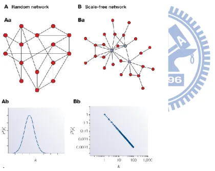
1.1.3 Scale-free distributions

Many scale-free networks are characterized by a power-law degree distribution [24] in

which the probability that a node has k links follows P(k) ~ k–γ, where γ is the degree

exponent. The probability that a node is highly connected is statistically more

significant than in a random graph(see Fig. 2, part Ba), with network properties often

determined by a relatively small number of highly connected nodes known as hubs. In

the Barabási–Albert scale-free model network model [24], a node with M links is

added to the network at each time point and connects to an already existing node I

with probability





, where k is the degree of node I and J the index

denoting the sum over network nodes. The network generated by this growth process

8

distribution represented by a straight line on a log–log plot (see Fig. 2, part Bb). The

network created using the Barabási–Albert model [24, 25] does not have an inherent

modularity, meaning that C(k) is independent of k. Scale-free networks with degree

exponents 2<γ<3(a range that is observed in most biological and non-biological networks) are ultra-small, with average path lengths that follow l ~ log log N. This is

significantly shorter than log N, which is characteristic of random small-world

networks [21].

Fig. 2. The comparison between the random network and the scale-free network.

1.2 Complex Network Structure

1.2.1 Motifs

9

graphs (G) at a number that is significantly higher than in randomized versions (i.e. in

graphs with the same number of nodes, links and degree distribution as the original

one, but where the links are randomly distributed) [16, 26]. As a pattern of

interconnections, M is usually expressed as a connected (undirected or directed)

n-node graph that is a subgraph of G. All the possible three-node connected directed

graphs are illustrated in Fig. 3.

ID 1 2 3 4 5 6 7 8 9 10 11 12 13

Motif

Fig. 3. 13 possible of triad motifs defined by Alon.

The concept of motifs was originally introduced by Alon et al.[16] who studied small

n-node motifs in biological and other networks. Significant motif research in a G

graph consists of matching algorithms – that is, counting the total number of

occurrences of each n-node subgraph M in the original graph and in the randomized

graphs. The statistical significance of M is then described in terms of Z-score, defined

as rand n rand M M M M

n

n

Z











Where nM is the number of times subgraph M appears in G, and  

rand M

n and _nrand

M



10

11

1.2.2 Communities

Community and the first network formalizations of the concept were proposed by

social scientists. Given a graph G(N, L), a community (or cluster, or cohesive

subgroup) can be expressed as subgraph G (N‘, L‘), whose nodes are tightly

connected, i.e. cohesive. Since the structural cohesion of the nodes of G quantified in

several different ways, there are different formal definitions of community

structures(Fig. 4)[27-29].

Fig. 4. Communities can be defined as groups of nodes such that there is a higher density of edges within groups than between them.

1.2.3 Hierarchical modularity

12

in many real systems, one must assume that clusters combine in an iterative manner to

generate hierarchical networks (Fig. 5, part A). The starting point for such

construction is a small cluster of four densely linked nodes (e.g., the four central

nodes in Fig. 5, part A). Next, three module replicas are generated and three external

nodes of the replicated clusters are connected to the central node of the old cluster,

thereby producing a large 16-node module. After generating three replicas of this

16-node module, the 16 peripheral nodes are also connected to the central node of the

old module, producing a new 64-node module. The hierarchical network model

seamlessly integrates a scale-free topology with an inherent modular structure by

generating a network that has a power-law degree distribution with degree exponent γ

= 1 + n4/n3 = 2.26(see Fig.5, part B) and a large, system-size independent average

clustering coefficient <C> ~ 0.6. A hierarchical architecture implies that sparsely

connected nodes are part of highly clustered areas, with communication between the

different highly clustered neighborhoods being maintained by a few hubs (see Fig. 5,

13

Fig. 5. The hierarchical network and its degree distribution.

1.3 Network Dynamics

Since actual complex networks are not necessarily static, simulating and/or studying

the dynamics of the complex networks is a difficult task. The following methods can

be used to address this problem in different domains.

1.3.1 Cellular automata

Cellular Automata (CA) [31]are simple examples of discrete dynamical systems. A

cellular automaton consists of a regular cell grid consisting a finite number of states.

Each ell state during time step t+1 is determined by states of cells in time step t. In the

14

bit-string CA) can be defined using the update rule defined in Table 1. In this example,

the state of a cell is determined by its own state and the states of its nearest neighbors.

This type of automaton can easily be schematized as a directed network in which each

cell takes inputs from two neighboring cells.

The time evolution of the cell states occur in discrete time steps with synchronous

update. Cellular automata are used to model several phenomena (e.g. pattern

formation) and to study various complexity theory concepts. Many types of cellular

automaton have been proposed, including random Boolean network and random

threshold networks. Three-cell block (t) 000 001 010 011 100 101 110 111 Center-cell (t+1) 0 1 0 0 1 1 1 0

Table. 1. An update rule for a one-dimensional, two-state cellular automaton.

1.3.2 Preferential attachment

15

connected nodes. Hubs are generated via ‗a rich-gets-richer‘ mechanism consisting of

growth and preferential attachment: the more connected a node is, the more likely

new nodes will link to it, meaning that highly connected nodes acquire new links

faster than their less connected peers. This mechanism ensures simultaneous the

16

Chapter 2 Static Networks and Dynamic

Process Characterization and analysis

No network in nature or technology is totally random—in other words, other

non-random mechanisms shape their evolution. The universality of various

topological characteristics, from degree distributions [25] to degree correlations [5,

22], motifs [16], and communities [2, 32], can be used as a springboard for studying

diverse phenomena and making predictions. Network theory has therefore

fundamentally reshaped our understanding of complexity. Even though researchers

still lack a universally accepted definition of complexity[32], the role of networks in

this area is obvious: all complex systems, from cells to the Internet and from social to

economic, consist of an extra-ordinarily large number of components that interact via

complex networks. We have long been aware of these networks, but only recently

have we acquired the data and tools to probe their topologies, thus giving us a clear

understanding of the strong impact of underlying connectivity on a system‘s behavior.

As a result, no single approach to complex systems can succeed unless it exploits

network topology.

17

behavior of systems that we perceive as being complex. We must be capable of

predicting how the Internet will respond to attacks and traffic jams, and how cells

react to environment changes. Progress in this direction demands an understanding the

dynamics of processes, a task made more difficult by the large number of dynamical

phenomena-almost as many as complex systems. Examples include the biological

study of reaction kinetics using metabolic networks, monitoring the flow of

information on computer networks; and exploring the spread of viruses and ideas via

social networks.

A major challenge is determining common characteristics among these diverse

dynamical processes. In this dissertation I will describe two approaches for

responding to this challenge:

For static networks, find relationships between network structure and function. I will

describe such relationships for two types of motifs in Chapter 3, and for network

hierarchy in Chapter 6

For dynamic networks, find global rules during network evolution. I will discuss

friendship evolution using three-rule model in Chapter 4 and epidemic dynamics with

18

2.1 Network Motif Detection

Commonalties have been found by complex network researchers in fields ranging

from biology to social and computer sciences. Three global features in complex

networks have been identified and investigated: highly clustered connections [1, 5],

small-world properties [1, 21], and the scale-free phenomenon [5, 7]. Approaches

based on quantitative and qualitative analyses of the topological properties of

complex networks are serving as the basis for studying how the global features of

network topological structures affect the dynamic behavior of networks [16, 33, 34].

This is currently considered one of the field‘s most important and challenging research topics [35, 36].

Some local structural motifs (also referred to as building blocks) reveal unique and

statistically significant patterns when compared with random [16], biological [1], and

food web [16, 26] motifs; all are perceived as containing important information.

However, the simple motifs of complex networks that are statistically significant but

functionally unimportant are inadequate for investigating network functions and

dynamic behaviors [16, 26]. In this dissertation, I will describe an algorithm that

19

and (b) identifies functionally and statistically significant network building blocks

from complex networks [37].

When considering the global features and local structural motifs of biological

networks, it is worth noting that link properties (weights) exert strong impacts on

network functions and dynamic behaviors [38-42]. Examples include the role of weak

links associated with the six degrees of separation (i.e., small-world) effect of

interpersonal networks [40, 41], and the strength of predator-prey interactions that

determine the stability of ecological communities [38]. Network researchers have

reported that weighted values representing interaction strength can be assigned to all

links (edges) in a real network [39, 43, 44]. I therefore considered network motif link

strength in terms of bridge motifs (consisting of weak links only or a minimum of one

weak link) and brick motifs (consisting of strong links only) (Fig. 6). Network motifs

can be separated into two categories: bridge and brick. Using the three-point

feed-forward motif as an example, it can be divided into two categories: a three-point

feed-forward brick motif (left box) composed of three strong (red) links, and a

three-point feed-forward bridge motif (right box) composed of at least one weak (blue)

link and a maximum of two strong (red) links as Fig. 6 shows. Bridge motifs connect

20

phenomenon of local clustering in biological networks.

21

2.1.1 General: Bridge and Brick Network Motif-Detecting

Algorithm

As shown in Figure 7, a link-weighted value that is dependent on the number of all

possible paths between two linked nodes equals the summation of the reciprocal

values of all possible path lengths except for the link itself. This is expressed as



where pathI(a, b) indicates the i th path from node a to node b; pathi(a, b) ≠ edge(a, b);

and length(pathi (a, b)) ≤ average network diameter. The length of one path represents

its total number of nodes.

Average network diameter =

2 ) 1 | (| | | ) , ( ,  



ShortestPath(a, b) = Min(length(pathi (a, b)))

22

(a, b) of edge (a, b) is 0 while weight (b, c)

This definition implies clustering, with any increase in the number of possible paths

resulting in an increase in the clustering degree between two linked nodes.

Furthermore, the concepts and algorithms discussed in this dissertation are

generalizable to non-directed networks. To ensure that the proposed method can be

applied to any complex network, the link-weighted values calculated by the network

motif detection method are derived from the number of all possible paths between two

linked nodes within all network topological and local connection structures (no preset

link quantity). This definition is similar to that of betweenness [43, 45]—effects

resulting from the removal of network links. Accordingly, the proposed link-weighted

value calculation method is assumed to represent the importance of each link in a real

network [46, 47].

Also considered were the interactive strengths of individual links in a quantitative real

network. To validate the proposal for weighted links, they were compared with

quantitative links. However, interactive quantitative links are defined by

category-specific functions such as proteins, genes, species, and so on. It is difficult to

specify the overall impacts of these links on protein-protein interaction networks [48]

23

not reflect the significance of their connection within an overall food web.

Furthermore, each complex network type has its own measure for interactive strength.

A switching algorithm (i.e., AB, CD becomes AD, CB if AD and CB do not exist) was used to create random networks according to any given degree

sequence [16, 26]. Results from previous studies indicate that these random networks

have the same number of nodes and edges, as well as node in-degrees (incoming

edges) and out-degrees (outgoing edges) that are identical to those of real networks.

Furthermore, randomized networks preserve the same number of appearances of all

(n-1) node subgraphs as in real (original) networks [16]. The threshold that

determines the strength of an edge (link) is the mean weighted value of all edges in a

random network ensemble. Accordingly, 1,000 random networks were generated to

serve as a control. Edges were labeled ―weak‖ when their weighted values in these or real networks were smaller than the threshold minus a double standard deviation (p =

0.01); all other edges were labeled ―strong.‖ Researchers can define criteria for strong and weak links according to their own needs. Finally, all possible motifs were located,

and their distributions in real and random networks were compared.

Milo et al.‘s method [16] for identifying bridge and brick motifs in complex networks was expanded to include the following steps:

24

1. Calculate the weighted value of each link in a network of interest and an ensemble

of random networks to calculate the significance of n-node subgraphs. The goal is to

maintain the same number of appearances for all (n – 1) node subgraphs as in the

original network.

2. Label all weighted links in the network of interest and random network ensemble as

―strong‖ or ―weak‖ according to a benchmark of two standard deviations from the mean weighted value of all links in the ensemble. Links with weighted values below

the benchmark are considered weak.

3. Identify all n-node bridge/brick subgraph types in the network of interest and

random network ensemble.

4. Mark all n-node bridge/brick subgraph types by calculating their numbers in the

network of interest and random network ensemble. Each n-node bridge/brick

subgraph type is selected as a representative motif only if its frequency in the network

of interest far exceeds its frequency in the ensemble.

These steps can assist research efforts to understand the functions and roles of

identified motifs in a real network and to analyze the dynamic behaviors of complex

networks. Regarding method robustness, the proposed approach emphasizes the

25

functions of different network types.

Motif frequency can be used to measure levels of similarity between two networks of

interest. In addition, it is possible to calculate the Z-scores for all bridge/brick motifs

and significance profiles (SPs) in a network by expanding Milo et al.‘s [26, 49, 50] methods. As shown in the following formula, ZScore(Bridgei) represents the statistical

significance of the ith kind of bridge motif in a network:

( ) ( ) ( ) ( ( )) real i random i Score i random i N Bridge N Bridge Z Bridge STD N Bridge     (2.3)

where Nreal(Bridgei) represents the time of appearance of the ith type of bridge motif in

a network, and <Nrandom(Bridgei)> and STD(Nrandom(Bridgei)) respectively represent

the mean and standard deviation of the time of appearance of the ith type of bridge motif in a randomized network ensemble. In the next equation, SP(Bridgei) is the

vector of ZScore(Bridgei) normalized to a length of 1. This normalization emphasizes

the relative significance of the ith type of bridge motif rather than the absolute significance. ZScore(Bricki) and SP(Bricki) can be derived in the same manner:







(

)

(

)

(

)

(

(

))

N

Brick

N

Brick

Z

Brick

STD N

Brick

 





26





(

)

(

)

(

)

Z

Brick

SP Brick

Z

Brick





2.1.2 Specific: Bridge and Brick Network Motif-Detecting

Algorithm

The previous method we proposed has solved some problems in different domains

successfully. However, since the concept of ―neighborhood‖ is very useful for

identifying the motifs or modules in biology. Another version of bridge and brick

network motifs is proposed for this specific domain. To ensure that the concepts and

methods described in this paper can be applied to any complex biological network, the

link-weighted value Link(v, w) for any edge between nodes v and w is expressed as its

hypergeometric coefficient Cv,w [51]. This value, which is frequently used to measure

cluster enrichment and co-occurrence significance, is expressed as:

min( ( ) , ( ) ) , ( ) ( )

( )

( )

( )

( , )

log

( )

T

N v

N v

N w

i

i

Link v w

C

T

N w











 





_{ }

_

_



 





 















where |N(x)| is the neighborhood size of node x and T the total number of nodes in the

27

can be represented as the probability of obtaining a number of mutual neighbors

between nodes v and w at or above the observed number when the neighborhoods are

independent. The hypergeometric coefficient Cv,w is consequently defined as the

negative log of this summation. Given the neighborhood sizes of the v and w nodes

and the T total number of nodes in the biological network, the higher the value of Cv,w,

the higher the number of overlapping neighbors between v and w—an indication that

Link(v, w) has a higher clustering coefficient. Otherwise, it does not belong to any

specific cluster (Fig. 8). Different link definition differs between the general algorithm

and the specific algorithm for detecting bridge and brick motifs, other parts are all the

same.

Fig. 8. The small-world model. Black signifies strong links and red weak links.

2.2 Social Network Simulation

28

The first rule addresses how people make new friends (via introductions or

meetings-by-chance), and the second rule addresses how friendships are broken when

one party dies. The model entails a fixed number of N nodes and undirected links

between pairs of nodes representing individuals who know each other [53]. To reflect

friendship weakening and strengthening, I added a ―friend remembering‖ rule (Fig. 9). The model repeats the following three rules until the acquaintance network in

question reaches a statistically stationary state:

Rule 1 (friend making). Randomly chosen individuals introduce two friends to each

other. If this is their first meeting, a new link is formed between them. Randomly

chosen persons with less than two friends introduce themselves to one other person at

random. Note that the term ―introduce‖ is used to describe meetings by chance as well as meetings via a common friend.

Rule 2 (leaving and arriving). At a p probability, a randomly chosen individual and all

associated links are removed from a network and replaced by another person.

Accordingly, acquaintances can be viewed as circles of friends whose members can

leave for reasons other than death and enter the circle for reasons other than birth.

Rule 3 (friend remembering). A certain number of friendships are updated, with the

29

explained in detail in the following two sections.

Fig. 9. Three-rule model flow diagram.

2.3 Epidemic Dynamics Analysis

The state transfer concept of SIS models adopted by Pastor-Satorras [54, 55] was

applied as the core simulation model architecture. Parameters were incorporated to

simulate behavioral and transformative results arising from agent interactions [56-60].

Each agent (node) in a complex network owns a set of properties and behavioral rules

that are used to demonstrate the features and statuses of persons in social networks or

computers connected to the Internet. A link between two nodes means that the

30

interaction/communication channel. An infectious disease or computer virus can be

transmitted via this link. At each discrete time step, the epidemiological state of each

node is determined by its behavioral rules, original epidemiological state, neighbors‘

epidemiological states, infection rate, and recovery rate. As stated above, ρ(t) is

defined as the density of infected nodes present during time step t. When time step t

becomes infinitely large, ρ can be represented as a steady density of infected nodes. A

computational flowchart for the proposed simulation model is shown in Figure 10. A

complex network G(N, M) with N nodes and M links was constructed using the

algorithm described previously prior to setting relevant parameters and attributes for

the nodes involved in the simulation; discrete time t was set at 0. During simulations,

nodes take turns interacting with neighboring agents for specified time intervals. Note

that individual agent interactions do not result in immediate influences, and that

simultaneous state changes only occur when all agents in a complex network

complete their interactions. Accordingly, interaction sequences do not influence

interaction processes or results.

At the beginning of each discrete time step, the usable economic resources of each

agent vi are reset to R(vi), meaning that all agents renew and/or receive supplemental

31

of sleep. In our later experiments, the statistical distribution of individual economic

resources could be delta (rConstant), uniform, normal, or power-law, as long as the mean

value <r> satisfied: t Cons N i i r N v R r 1 _tan ) (   



At each discrete time step, each vj agent interacts with one agent selected from all of

its Neighbors(vi). After the interaction process is completed, agents vi and vj must

have transmission costs c(vi) and c(vj) (0 ≤ c(vi) ≤ R(vi) and 0 ≤ c(vj) ≤ R(vj)) deducted

from their respective economic resources, regardless of the interaction result. If R(vi)

< c(vi) after the interaction, agent vi cannot interact with other neighbors because all

of its resources have been used up. Otherwise, it repeats the interaction process by

choosing another neighboring agent until its resources are exhausted.

Assume that infected and contagious agent vi is adjacent to susceptible and

infection-prone agent vj. When the two agents come into contact, a combination of

infection rate RateInfect, agent vj‘s resistance level, and a random number r

determines whether or not vj is infected by vi. If the random number r is lower than

the infection rate RateInfect, agent vj‘s epidemiological state becomes I (Infected).

32

recovery rate. Without a lack of generality, recovery rate RateReset can be assigned as

1, meaning if agent vj is infected by other agents at discrete time step t – 1, it will

recover and once again become susceptible at discrete time step t, since it only takes

affect according to the definition of the infection disease propagation time scale. At

the beginning of an infectious disease simulation, only ten individuals were given I

status; all others were given S(Susceptible). During each time step, agents randomly

interacted with several neighbors. All epidemic experiments discussed in this paper

33

Fig. 10 Flowchart for a SIS epidemiological simulation model.

2.4 Abstraction Hierarchy

The proposed two-way method is considered novel because it emerges from top-down

and bottom-up clustering algorithm synergy [61, 62]. Not only does it identify

modules in a top-down fashion and construct a hierarchy implied in a complex

34

at different levels in the hierarchy. The method consists of three steps: (i) computing

between-node proximity, (ii) extracting the backbone(represented by a spanning tree)

from the network and using it to partition the network [28, 63], and (iii) generating an

abstract network. Iteratively applying the same steps to a newly generated abstract

network supports the discovery of an abstraction hierarchy within a complex network

[2, 64].

2.4.1 Proximity Measure

Proximity between two nodes can be defined in many ways; since it affects resulting

module formation, selecting an appropriate proximity function is very important.

Commonly used measures include Euclidean distance, correlation coefficient and

cosine similarity [65, 66]. Module analysis is problem-dependent as stated earlier, in

this dissertation I investigate clustering based on network topology. Conventional

proximity measures are not applicable to clustering problems if network topology

represents the only available information-that is, Euclidean distance cannot be

calculated without node coordinates. Other proximity measures( e.g. edge

betweenness [45] and topological overlap[65, 67, 68]) have recently been proposed

35

While some successful applications have been reported, they have at least two

limitations: (a) edge betweenness of node pairs reflects the global characteristics in a

network, but they suffer from high computational costs [64] and are affected by the

network incompleteness and noise [32, 64]; and (b) sine topological overlap is a local

measure, it poses a challenge to identifying any module beyond a locally dense

connectivity pattern [69].

Most proximity measures in current use do not take link direction or weight into

account. Therefore, any directed weighted network is processed as an undirected

unweighted one. To expand its applicability, I propose using a new proximity function

for dealing with directions and weights. For the sake of simplicity, I will describe a

directed weighted network of n nodes by an nn adjacency matrix A, in which each element Aij is the weight of the link from node i to j. A zero-valued weight (Aij=0)

indicates the absence of a link between those nodes. The proximity function prox(i,j)

from node i to j, i  j is defined as:





36

function considers not only the effects of common neighbors (i.e. node k), but also

link direction and weight. It treats the direct link from node i to j differently than

indirect paths between the same nodes through a common neighbor k. The weight of

the direct link contributes to prox(i, j), as indicated by the first term in the above

equation. To calculate i-to-j proximity based on an indirect path from i to j by way of

k, I divided the path into two sub-paths, from i to k and from k to j. Assuming on an

indirect path one node does not always affect all its neighbors, but instead acts

probabilistically. Thus, the probability that one node affects another(e.g. i affects k) is

defined as the ratio of the link weight between them to the sum of the weights of all

outgoing links from node i, not including the direct link from i to j. The probability of

an indirect path from i to j by way of k is therefore the product of the probability of

paths from i to k and the path from k to j. The proximity between i and j contributed

by the indirect path ikj is assigned to the probability times the minimum of Aik and

Akj. In cases where there is more than one common neighbor of i and j, the sum of the

proximity of each indirect path is used.

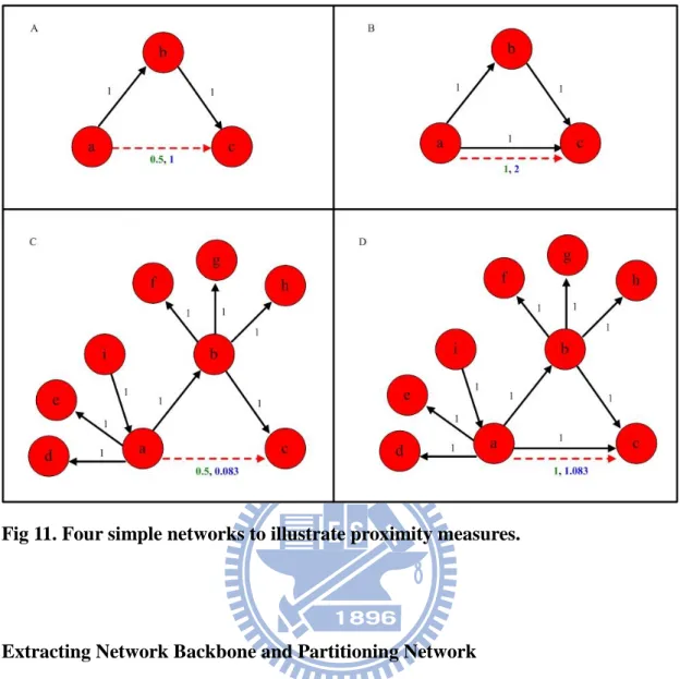
The examples shown in Fig. 11 illustrate our proximity function and compare it with a

related measure, topological overlap [67, 68, 70]; both take common neighbors into

37 defined as follows:  T_ij  lijaij min( d_i,d_j)1a_ij , (2.10)

where lij is the number of common neighbors shared by node i and j, di is the degree

of node i, and aij=1 if a direct link exists between i and j (otherwise, aij=0). The 1- aij

quantity in the denominator prevents the denominator from becoming zero in case

where min(di,dj)=0. The inclusion of aij in the numerator is to make Tij explicitly

dependent on the direct link between i and j.

Given the network in Fig. 11A, Tac=0.5 and prox(a,c)=1. To evaluate the effects of

direct links, one direct link was added between nodes a and c (Fig. 11B). If we

compare the network to a gene regulation model, a can be interpreted as a regulator, b

as an intermediate gene, and c as a target. Since gene a can regulate gene c either

directly, or through the intermediate gene b, the proximity between a and c in Fig.

11B should be higher than that in Fig. 11A. Increase in proximity were found in both

measures-that is, Tac=1 and prox(a,c)=2 vs. Tac=0.5 and prox(a,c)=1. The network

shown in Fig. 11C is different from the one in Fig. 11A in that node a and b both have

more neighbors. Considering the network as a model of gene regulation, it means that

38

of gene a on gene c may be diminished. For node a and node c in Fig. 11C, prox(a,c)

decreases to 1/12, which corresponds reasonably to the gene network model. In

contrast, according to the topological overlap measure, the proximity between nodes a

and c is 0.5, which is the same as that in Fig. 11A. Topological overlap measure fails

to distinguish between Fig. 11A and 11C. To complete the illustration, we added one

direct link between a and c, and created the network shown in Fig. 11D. An increase

in proximity results from either measure.

Even though the proposed proximity function is a local measure(similar to topological

overlap), it shows better discrimination in network topology and requires less in

computational costs than global measures such as edge betweenness. Incorporating

the proximity function into a two-way module-finding and hierarchy-building strategy,

it is possible to gather global characteristics and to detect the hierarchical structure of

a network. We validated our approach using hierarchically nested random networks as

39

Fig 11. Four simple networks to illustrate proximity measures.

Extracting Network Backbone and Partitioning Network

An optimal solution for network partitioning (based on a criterion function) emerges

after enumerating all possibilities, but it is computationally prohibitive for large

networks. In response to this problem, a graph-theoretic approach to partitioning was

adopted [71]. After computing the proximity between all node pairs, it is possible to

build a maximum spanning tree that includes all network nodes, which are all

40

proximities are discarded, the maximum spanning tree acts as the network backbone.

To reduce computational costs, partitioning is performed based on the maximum

spanning tree instead of the original network.

Two subtrees can be obtained by removing one link from a tree, with each subtree

representing one module. One tree can be partitioned into many subtrees (i.e.

modules/clusters) by repeating the same process on each subtree. Given the maximum

spanning tree, resulting modules can be examined by removing one link from a

(sub)tree. A link is selected for removal if the M={M1,M2,M3,…,Mn} set of modules

meets the following criteria after removal:





M

,M



M, a



b S



S



S



S



S



is the sum of the proximity of each intralink within Mk, and



S



is the sum of the proximity of each interlink between Ma and Mb.

These criteria for modules are similar to those described in [64] and [72], except that

link weight (i.e., proximity) is considered instead of node degree. The simple example

network shown in Fig. 12 demonstrates the advantage of using the link weight criteria.

Without taking the weight into account, intuitively the most appropriate partition of

the network is to cut the link between node C and node F, and obtain two modules.

41

nodes only, the simple network will be partitioned in the way above. However, in

practice, if the weight represents the significance of connectedness, the network

should be considered as a whole. Our criteria for modules take weights into account;

therefore, the network cannot be divided based on our criteria. In the case of an

unweighted network, by treating each link as one with a constant weight, e.g. one, this

simple network will be partitioned into two modules as expected according to our

criteria. Without losing generality, this simple network demonstrates that our criteria

for modules are more realistic, and can subsume the previous definitions of modules

[72]. Note that the proximity sum is calculated for the network rather than the tree,

thus preventing information loss. In the proposed model, the tree is only used for

evaluating which nodes may form clusters, thus reducing the search space of the

original network.

42

Pseudocode for the partitioning procedure is shown below, starting with a single

module represented by a maximum spanning tree. The input includes the network Net

in question; M1 is its maximum spanning tree. The output consists of partitioning

result in clusters.

Procedure Network_Partition (Net, M1)

M={M1} //M keeps the modules for further analysis

Repeat

{

Select a cluster Mi M, and remove Mi from M.

Put Mi into D. //D stores the final clusters

Put all the links of Mi in Li.

While (Li is not empty)

{

Set the link in Li with min proximity as lmin.

Remove lmin from Li.

43

Add Ma and Mb to M.

If M does not satisfy criteria [4]

{

Remove Ma and Mb from M.

Restore lmin to Mi. //put the link lmin back to the tree Mi

}

Else

{

Remove Mi from D. // because Mi is legally split into Ma and Mb

Break; //break out of While loop

}

} until M is empty.

Output D.

2.4.2 Network Abstraction

After the partition of the network, each module is treated as a supernode [7, 73] and a

network of the supernodes is viewed as an abstraction of the original network. An

abstract network reveals the general framework of the original network without any

44

module Ma and Ma) is defined as





M

M

prox

m

n

prox

(

,

)

(

,

)

where |Ma| is the number of nodes in module Ma. Proximity between all possible

supernode pairs are computed and normalized to a z-score. Links that have z-scores

below a pre-set threshold are considered insignificant and therefore discarded. The

resulting supernode network (an abstraction of the original network) is placed one

level higher than the original network in the hierarchy. By repeating the same process

with other networks in the hierarchy, it is possible to generate additional abstract

networks and to consistently and systematically build a pyramid of abstraction from

45

Chapter 3 Network motif Experiments

Researchers are making progress toward defining organizing principles that govern

the formation and evolution of complex biological networks. Considered a major

challenge in computational system biology, predicting network behaviors [74] and

functions requires the identification of functionally and statistically important motifs.

To understand their structural organizing principles and evolutionary mechanisms,

bridge motifs can be defined as consisting of weak links only or at least one weak link

and multiple strong links; brick motifs can be defined as consisting of strong links

only. Next, an algorithm is proposed for performing two simultaneous tasks: detecting

global statistical features and local connection structures in biological networks, and

locating functionally and statistically significant network motifs.

3.1 General: Bridge and Brick Network

Motif-Detecting Algorithms

Commonalties have emerged from studies of complex networks in fields ranging from

biology to social and computer sciences. Three global features in complex networks

46

75], small-world properties [21, 75-78], and the scale-free phenomenon [1, 24, 39, 79].

Approaches based on quantitative and qualitative analyses of the topological

properties of complex networks are being utilized to study how the global features of

network topological structures affect the dynamic behavior of networks [1, 39, 80-84]

39-40]. This is currently considered one of the field‘s most important and challenging

research topics [1, 39].

Some local structural motifs (building blocks) reveal unique and statistically

significant patterns when compared with random [16, 80, 85-90], biological [16, 87],

and food web [16, 38] motifs; all are thought to contain important information.

However, simple motifs of complex networks that are statistically significant but

functionally unimportant are clearly inadequate for investigating network functions

and dynamic behaviors [16, 82, 88, 90-93]. An algorithm is therefore proposed to

perform two tasks: simultaneously detect global features and local structures in

complex networks, and identify functionally and statistically significant network

building blocks from complex networks.

When considering the global features and local structural motifs of biological

networks, it is worth noting that link properties (weights) exert strong impacts on