Image Segmentation to Inspect 3-D Object Sizes

Jui-Pin Hsu Abstract. Object size inspection is an important task and has various Chiou-Shann Fuh

National Taiwan University

applications in computer vision. For example, the automatic control of stone-breaking machines, which perform better if the sizes of the stones Department of Computer Science and to be broken can be predicted. An algorithm is proposed for image

seg-Information Engineering Taipei, Taiwan

mentation in size inspection for almost round stones with high or low texture. Although our experiments are focused on stones, the algorithm E-mail: fuh@robot.csie. ntu.edu.tw can be applied to other 3-D objects, We use one fixed camera and four

light sources at four different positions one at a time, to take four images. Then we compute the image differences and binarize them to extract edges. We explain, step by step, the photographing, the edge extraction, the noise removal, and the edge gap filling. Experimental results are presented.

Subject terms: visual commurrictiions and image processing; image segmenta-tion; image difference; edge extraction; edge detection; gap filling.

Optical Engineering 35(l), 262-271 (January 1996).

1 Introduction 1.1 Motivation

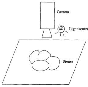
A typical stone-breaking machine has two rollers to squeeze and break stones, as shown in Fig. 1. To use the machine, we should adjust the space between the two rollers properly, according to the sizes of the stones. On one hand, if large stones come, we should adjust the space wider, or the lifetime of the rollers will be shortened; on the other hand, if small stones come, we should adjust the space narrower, or the stones will slip through, and electricity will be wasted. Hence, segmentation on stone images for size inspection isimportant if we want automatic control of the machine.

1.2

Sun?fmry

If the stones have some high-contrast texture, a traditional gradient edge detector will find many false edges. If the stones have almost no texture, it will be hard for a stereo image technique to match corresponding points.’ Similarly, a tra-ditional gradient edge detector will fail to find the edges between two stones with almost the same brightness. Thus we use four light sources to the north, south, west, and east of the camera, one at a time, to photograph images and then use image differences to detect the shadows, which occur at the edges, for edge extraction. The image differences are computed for each pair of images with light sources at op-posite sides, to extract edges in both north-south (N-S) and east-west (E-W) directions.

Some related works on edge detection are Refs. 2,3. They extract edges from a source image rather than from image differences.

PtIp~rVIS-115rccciwl M:IY N. 1995;~cvisc~IIl:lnuscrlp[recei,cclAug. 18,1995: 73 199.i.

JLUT@d tor puhlwm Au:, . . .

0 1996 Socie[y o! Pho[wOp[ic:d Insmnlmtil(ion Engimm. 009 I -3286/96/S6.00.

Treating image differences as edge responses, we binarize them to get binary edge images in both N-S and E-W direc-tions. Usually, a single-threshold scheme cannot acquire good edge images. We propose an original binarization scheme using local and global thresholds.

After the binarization comes the edge imaging, imple-mented as the binary OR of binary edge images in the N-S and E-W directions. After the edges are extracted, we remove the noise by connected-component analysis, to get a clearer edge image.

Due to some inevitable problems explained later, the ex-trdcted edges will not all be linked. General edge-linking techniques seem unable to solve the problem. A snake algorithrn5 or front propagation algorithm may fill the gaps but will fall into local minima, as shown in Fig. 2. We detect the terminals of edge pieces by a corner detector using a K-cosine algorithm,7’8 and we propose a terminal extension algorithm to fill the edge gaps. Some related proposals for corner detection are in Refs. 9 to 12. They may be chosen to improve performance in certain cases of segmentation, but we choose the original K-cosine algorithm for simplicity, and it suffices.

2 Setup for Photographing

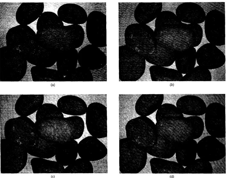
We are to take four images with four light sources to the north, south, east, and west of the camera, one at a time. Figure 3 shows the setup with the light source to the east (E) of the camera. The other light source positions are similar, and to the north (N), south (S), and west (W), respectively. The four source images are shown in Fig. 4, which was taken with a CCD camera with lens of focal length 25 mm. The resolution is 479H X 632W, and the distance between lens and the stones is about 62 cm. Each light source is about 7 to 8 cm away from the center of the lens. In our experiments, the sizes of the stones are about 5 X 5 X 2 to 8 X 6 X 5 cm. The light source is a frosted 40-W light bu]b, which provides

IMAGE SEGMENTATION TO INSPECT 3-D OBJECT SIZES

Stonesto bebroken.

o~o

Left roller. Righ roller.

Adjustab~ space between thetwo rollers,

Fig. 1 Side view of the rollers of a stone-breaking machine

--- Possible snake contour: bad shortcut at bottom-left comer.

Fig. 2 Snake algorithm will fall into local minima in some cases.

equal illuminance in all directions. Light bulbs of clear glass will generate uncontrollable patterned light and degrade the subsequent processing of image differences.

3 Algorithm and Experimental Results 3.1 Absolute Image Difference

Let the four source images be N, S, E, and W, corresponding to the images with light sources to the north, south, east, and west of the camera, respectively. We can see that the major differences between the four images are in the positions of the shadows. We compute the absolute image differences, IIN– Sl[ and /1.E– W]/, where 11.]1stands for absolute value, to extract edges from the shadows.

As we can expect, the absolute image difference IIN– Sll will have larger values at the horizontal edges of the stones, but smaller values at edges in other directions and non-edge pixels, since the shadows will differ at horizontal edges. Sim-ilarly, IIE – W1/has the same effect at vertical edges. Figure 5 shows the histogram equalized absolute image differences for viewing.

3.2 Local and Global Thresholding

To get binary edge images in both N-S and E-W directions, we binarize the absolute image differences. Using a single global threshold will result in edge images with large gaps between broken edge segments. Thus we combine local thresholding and global thresholding to extract edges and get edge images with small gaps.

For local thresholding, we define a local thresholding con-dition, to test if a pixel has its intensity a% higher than the average intensity of its local 13 X 13 window area or not. Those that pass the local thresholding condition will be

n

~t!!)

\ ‘l\

Fig. 3 Global view of the camera setup.

marked as white; the others as black. Applying local thresh-olding to IIN– S]1and IIE– W1/, we get two images, LTHRn, and LTHRCW, as shown in Fig. 6. The percentage @ is set to 20 in our experiments.

For global thresholding, we binarize images, with thresh-old at a little higher percentage (~%) than the expected per-centage (y70) of edge pixels. The percentage y is typically about 15, and ~ is set to 22 in our experiment. That is, the brightest 22% of pixels will pass the global threshold con-dition and be marked as white, and the others as black. Ap-plying global thresholding to IIN – Sll and (IE – Wll, we get two images, GTHRnS and GTHRCW, as shown in Fig. 7.

To combine local thresholding and globa[ thresholding, we compute THRns and THR.W, as shown in Fig. 8, by the following equations:

THRI,, = LTHRn, AND GTHRns , THRCW= LTHR=WAND GTHR,W

Here AND denotes the binary AND operator.

To gather edge information on both the N-S and E-W di-rections, we compute the combined edge image, THRCo~billed, as shown in Fig. 9, by the following equations:

THRCo~bined= THRn, ORTHRC,V . Here OR denotes the binary OR operator.

We do not set the global threshold value at the exact percentage of edge pixels, not only because it is hard to know the exact percentage, but aIso because we rely highly on local thresholding, which extracts edges more effectively. Global thresholding only helps us to eliminate the false edges ex-tracted by local thresholding at pixels of small intensities. Thus a somewhat loose condition for globaI thresholding will allow more edge pixels, and aIso noise pixels, to pass the threshold, and leave them to be distinguished by local thresh-olding. Local thresholding is unstable at pixels of small in-tensities, since when the intensity is small, a little change in intensity will make a large change in percentage, and our local thresholding is based on relative intensity. In the local-thresholding results (Fig. 6), we can see many false edge

(b)

(d)

Fig. 4 Source images with light sources to four directions (a) N, (b) S, (c)E,and (d)Wto the camera The resolution is 479H x 632W

pixels at the locations with low intensities in image dif’fer-~nces (Fig. 5). However, the false edge pixels cannot paSS

the global threshold (Fig. 7) in either the N-S or the E-W direction.

Stones generally are very Lambertian. but not perfectly Lambertian. IIiurninating an object that is not Lambertian will result in bright spots in the image, caused by direct reflection of the light source. The positions of the bright spots change as the positions of the light sources change. Thus we will get significant image differences at the bright spot areas, and obtain false edges, if only a single global threshold is adopted. Because stones are very Lambertian, the intensity of pixels in bright spot areas will change smoothly. Thus pixels in bright spot areas cannot pass the local thresholding condition, and will be marked as non-edge pixels. We can see many false edge pixels in globa[ threshokling results (Fig. 7) in bright spot areas of the source images (Fig. 4). However, the false edge pixels cannot pass local threshold (Fig. 6) in either the N-S or the E-W direction.

For choosing the parameter CX,the stronger the contrast between shadows and stones in the source image is, the better

the edge image will be, and the higher the value at which u can be set. Specifically, what we want to distinguish in the thresholding is the edge pixels and the non-edge pixels. In the absolute image differences, edge pixels come from dif-ferences in brightness between shadows and stones, while non-edge pixels come from differences in brightness between stones illuminated by light sources at different positions. Thus the parameter CLdepends on the contrast of the two differ-ences, while the two differences themselves depend only on the illumination, including the gray levels of the stones and the brightness of the light source. Thus the darker the stones are, the smaller the difference of the two differences will be, the worse the edge image will be, and ~he lower the value at which a can be set.

The parameter @can be set to a percentage a little higher than the expected percentage of edge pixels, and /3 has little effect, because global thresholding only helps local thresh-olding at the pixels of low intensity in image difference.

The window size for local thresholding depends on the thickness of the shadows, which depends on the thickness of the stones and the distance between the light source and the

IMAGE SEGMENTATION TO INSPECT 3-D OBJECT SIZES

(a)

(b)

Fig. 5 Histogram-equalized absolute image differences for viewing: (a) Hist (IIN- S11). (b) Hist(llE- Wll). Hist (.) stands for histogram equalization.

stones. The thicker the stones are and the shorter the distance between the light source and stones, the thicker the shadows will be, and the larger the window size should be set. In our experimental results, a window size of 7X7 is good, and can filter out much of the noise. For demonstrating possible noise spots, and some typical bad cases, we use a window size of 13X13.

3.3 Noise Removal for the Edge Image

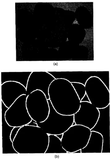
After the thresholding, the edge image has small spots of noise. For noise removal, we use the connected component algorithm on THRCon,bi,,.d to filter out small white compo-nents less than 40 pixels and small black compocompo-nents less than 400 pixels. The result image, EDGE, is shown in Fig. 10. We assumed that stones whose areas are smaller than 400 pixels do not exist. In practice, stones of such small sizes are unimportant and thus ignorable. Some noise components ex-ceeding 40 pixels may exist. This problem can be solved by a convex hull algorithm after the segmentation. We discuss it in Section 4.2.

Fig. 6 Local thresholding: Pixels 20% brighter than average bright-ness in the local 13x 13 area will pass the threshold and be marked as white. (a) LTHRns = LThr20.,d(IN– SI ), and (b) LTHR,W = LThr20.,o(IE– WI), where LThr20.,o () stands for our local thresh-olding with a =20.

3.4 Smoothing the Edge Boundaries and Using a K-Cosine Algorithm to Extract Edge Terminals The edge image has many gaps. Figure I I shows one of the reasons why edge gaps form. We trace the edge boundaries and find the edge terminals to fill the edge gaps.

For smoothness, we dilate each edge pixel in EDGE to all its eight neighbors, called EDGEtl,,C~, as shown in Fig. 12. This results in a little less accurate edge image; however, it provides more accurate K-cosine values for later processing.

Figure 13 shows the boundaries of edges. For each pixel along the boundaries, we compute the K-cosine values by tracing the boundary counterclockwise. Each edge pixel is classified as a left turn or right turn, according to the angle used to compute the K-cosine value. By thresholding

K-cosine values we can find corners, at which we select the right-turn pieces to be the terminal pieces of the edges, as shown in Fig. 14.

3.5 Terminal Extension to Fill Gaps

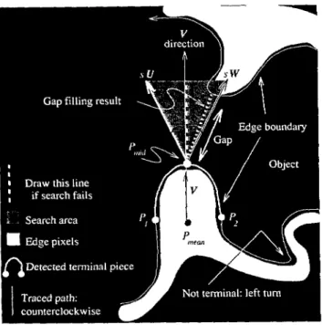
Let the two end points of the terminal pieces be PI and P2, the midpoint of the piece be Pmid, the midpoint of PI and P2 be P,,,,,,,,, and the vector V be Prnca,,P,,,i~ Let the two unit vectors U and W have angle + between each of them and V. We search the triangle spanned by SU and sW, where s is a scalar, to fill the gaps, as explained in Fig. 15. If a white pixel that is not locally connected to P,,,id is found in the triangle, we decide the space between the white pixel and

P,,,i,i is the gap, and directly link the white pixel to Prnid by

a straight line segment. Contrarily, if no white pixels are found in the triangle, we draw a white line segment from

P,,,id to the midpoint of the other side of the triangle, that is,

the altitude of the triangle from Pn,id. The result is shown in Fig. 16. The parameter + is set to 35 deg, ands is set so that the altitude of the triangle described above is 30, that is, s = 30 see+ =30 sec (35 deg)=36.6. Note that if a gap of length 50 is encountered, and the gap has two terminal pieces detected

IMAGE SEGMENTATION TO INSPECT 3-D OBJECT SIZES

Fig.10 EDGE, noise-removed edge image: White connected com-ponents less than 40 pixels and black connected components less than 400 Pixels inTHR.omtxned are filtered out.

Light sourcel Light source2

“’;$$ .?. _,.”

-...

,..

Tan~ent line Tangent line

Fig. 11 No shadow exists under each of the two light sources at the same sides of both tangent lines, so no significant difference is on the pointed edge. Thus some edge pixels will not be detected, and edge gaps form,

by our aIgorithm, then the terlminal extension algorithm will extend the first terminal piece by 30, since the search for edge pixels fails. On the second terminal piece, the algorithm will search for and find the extension part of the first terminal, and then link them by a line segment, since the gap will be reduced to about 20 after the first extension. Thus the two line segments fill the gaps.

We can expect that the best chosen @ is independent of stone size, and a little dependent on gap size. In experiments, we find that @ is not sensitive to noise, stone size, or gap size, and can be set to a constant. The parameters depends on gap size. The larger the gaps are, the higher the value at which s should be set.

3.6 Removal of Un wanted Filling Line Segments

Fig. 12 Dilation of edge image to smooth edge boundaries

Some line segments for gap filling may be false. The un-wanted line segments are all thin, and the pixels on the thin line will have less white pixels in their neighborhood than

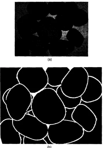
Fig. 17 The complete segmentation result unwanted line segments removed from the gap filling result.

normal thick boundary pixels, as illustrated in Fig. 16. Thus we can detect the pixels on the thin lines, and eliminate the ones that are not separators of any two or more regions. Figure 17 shows the result, and we complete the whole seg-mentation.

3.7 Biased Estimation

It should be noted that this method is a biased estimation, as shown in Fig. 18. Ordinarily, stones will not be perfectly round, so our object model consists of two arcs and two straight lines. The object model will shrink to a ball when L equals zero. The part of the object to the right of the tangent line L, will be in shadow under light source 1 but will be bright under light source 2. This part will be detected as edges. Similarly, the part to the left of Lz will be detected as edges.

C3mT!a

\’pf&~:?~:.!..Y

\\

“

Exact obtec: size = 2L + 2R _\ L~

L, Fig. 18 Geometrical and radiometric model.

Thus the size of the part of the object between the two tangent lines L] and Lz will be the measured object size (MOS). Since only the part of object between the tangent lines L3 and L4 can be viewed by a perspective camera, the size of this part will be the best measurable object size (BMOS). The exact object size (EOS) is 2L + 2R, The relations are as follows:

[(d, +L)2+Zfz-Rz][’1 sin+l=lt cos$l+L+dl , (1)

[(d2 + L)2 +H2 –R*]’” sin@2 =R cosr$2 + L+ d2 , (2)

MOS=R COS$, +R COS4Z+2L , (3)

[(d– L)z+H2– Rz]”z sinal =R Cosa.l +L–d , (4)

IMAGE SEGMENTATION TO INSPECT 3-D OBJECT SIZES

[(d+ L)2+H2– R2]1n sina2=R Cosaz +L+d , (5)

BMOS=R COSCJ., +R COS(12 -t-2L , ₍₆₎

d] – d2 d=—

2“ (7)

In some cases other than that in the figure, when the related positions of the camera, the light, and the object differ, the formulas may differ in certain signs (plus or minus) for some certain terms. The relations are a little complex. Some typical parameters for the bias are listed in Table 1.

3.8 Performance

The algorithm above is implemented on a Sun SPARCstation 10 machine. Although the program is not optimized, it can still complete the work in 50 s. In fact, it should be done in 7 s, including the computation of the stone size, which is not included in this paper. The time can be shortened still further by better hardware, an optimized program, or perhaps a par-allel program on a parallel computer. More experimental results are shown in Figs. 19 to 23.

4 Conclusion and Future Work 4.1 Conclusion

We have proposed an algorithm, including picture photo-graphing, edge extraction, noise removal, and edge gap fill-ing, for stone image segmentation. Our key idea is to use image differences to be able to process typical stones with both high and low texture. For edge gap filling, we make use of a K-cosine algorithm to find edge terminal pieces.

Black stones whose brightness is very similar to that of the shadows cannot be processed successfully by this algo-rithm, since we use the image difference between brightness of stones and shadows to detect edges. Similarly, it is also hard to detect edges of black stones with human eyes. The stones to be broken are usually brown or gray in the real world. Another application is to break stone-shaped concrete pieces, which are not black either.

Table 1 Typical parameters versus error rates: the B rate stands for (MOS – BMOS)/BMOS, and the E rate stands for (MOS – EMOS)/EMOS.

Free Variable Constrained Variable Error Rate

H L R dl dz d rjl ~~ al ct~

Mos

62 1.5 1 8 8 0 0.168 0.168 0.040 0.040 4.972 4.998 5.000 -0.5% -0.5%

62 1.5 1 9 7 1 0.184 0.152 0.024 0.056 4.971 4.998 5.000 -0.5% -0.6%

62 0.5 2.5 8 8 0 0.151 0.151 0.024 0.024 5.941 5.999 6.000 -0.9% -1.0% 62 0.5 2.5 10 6 2 0.182 0.119 -0.008 0.056 5.941 5.996 6.000 -0.99?0 -1.0% 62 0.5 2.5 18 -2 10 0.301 -0.008 -0.137 0.182 5.887 5.935 6.000 -0.8’?ZO -1.9’%0

(a)

(b)

the results only slightly, and is less critical. For estimating a automatically, the discussion of the principles for its choice in Section 3.2 may be helpful.

To estimate sizes of stones, which is one direction for future work, we should first estimate the missing edges and occluding edges. Although the line segments for gap filling cannot represent the true edges of the stones, we can retrace the edges of the stones after the segmentation, and use the resulting edge information, except the line segments, to es-timate the missing edges, including the improper line seg-ments and the occluded edges. The analysis of these edges

will help to eliminate the small noise spots of size exceeding 40 pixels mentioned in Sec. 3.3. After all this, sizes of the stones can easily be estimated.

Acknow/edgmerfts

This research work was supported by National Science Coun-cil of Taiwan, ROC, under NSC grants NSC 83-0422-E-O02-010 and NSC 84-2212-E-002-046, and by Cho-Chang Tsung Foundation of Education under grant 84-S-26.

References

1. R. M. Hamiick and L. G. Shapiro, CompI/fer md Robof Vision, Vol.

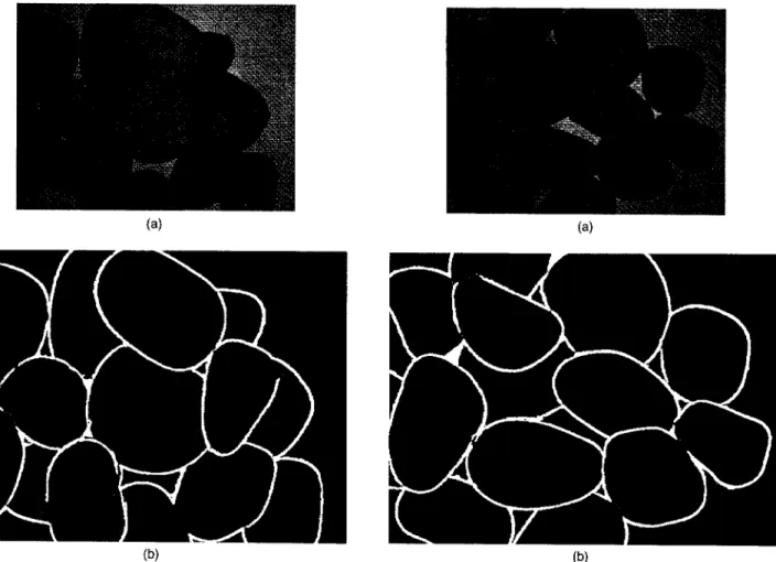
Fig. 21 Experiment 3: (a) one of the four source images; (b) the segmentation result.

2, pp. 357-362, Addison-Wesley, Reading,MA, 1993.

2. K. R. Rao andJ. Ben-Arie, “Optimal edge detection using expansion matching and restoration,” IEEE Tram. Pattern Anal. and Muchine

lnre//. 16(12), 1169-1 [82 (Dec. 1994).

3. F. van der Heijden, “Edge and line feature extraction based on co-variance models, ” IEEE Trans. Pattenz Anal. md Machine lnteli. 17( 1), 16-33 (Jan. 1995).

4. R. C. Gonzalez and R. E. Woods, Digifa/ Inqe F’rrx’e.wing, pp. 429-443, Addison-Wesley, Reading, MA, 1992.

5, F. Leymarie and M. D. Levine, “Simulating the grassfire transform using an active contour model, ” IEEE Trans. Puttern Anal. mrd MLI-chine he//. 14( I), pp. 56–75 (Jan. 1992).

6. R. Malladi, J. A. Sethian, and B. C. Vemuri, “Shape modeling with front propagation: a level set approach,” IEEE Tram. Parrern Anal. wrd Machine Intel/. 17(2), 158–175 (Feb. 1995).

7. A. Rosenfeld and E. Johnston, “Angte detection on digital curves,”

IEEE Trm.s, Conynrt. C-22, 875-878 (Sep. 1973).

8. A. Rosenfeld and J. S. Weszka, “An improved method of angle detec-tion on digital curves,” /EEE Tmrr.s.Compur.24,940-941 ( 1975). 9. X. Li and N. S, Hall, “Corner detection and shape classification of

on-line hand-printed kanii strokes,” PnrrcrnRecognition 26(9), 1315-1334

(1993).

-10. W. Y. Wu and M. J. Wang, ‘‘Detecting tbe dominant points by the curvature-based polygonal approximation,” CVGIP: Graphical Models and hnagc Process,55(2), 79-88 ( 1993).

1I. A. Rattarangsi and R. T. Chin, ‘‘.%ale-bdSed detection of corners of planar curves,” IEEE Trans. Pmrern Anal. and Machine Inteli. 14(4), 430zt49 (Apr. t 992).

12. S. J. Wang and C. S.Frrb, “Adaptive dominant point detection via the rated composite vectors,” Master’s Thesis, Dept. of Computer Science and Information Engineering, National Taiwan Univ., Taipei, Taiwan (June 1994).

IMAGE SEGMENTATIONTO INSPECT 3-D OBJECT SIZES

(a) (a)

(b) _(b)

Fig. 22 Experiment 4: (a) one of the four source images; (b) the segmentation result.

Jui-Pin Hsu received the BS degree in mathematics from National Taiwan Univer-sity, Taipei, Taiwan, in 1992, and the MS degree in computer science and informa-tion engineering from the same university in 1995. He is now a lecturer in Foo-Yin Ju-nior College of Nursing and Medical Tech-nology, Kaohsiung, Taiwan. His current research interests include image segmen-tation, image reconstruction, and computer vision.

Fig. 23 Experiment 5: (a) one of the four source images; (b) the segmentation result.

Chiou-Shann Fuh received the BS de-gree in computer science and information engineering from National Taiwan Univer-sity, Taipei, Taiwan, in 1983, the MS de-gree in computer science from the Penn-sylvania State University, University Park, in 1987, and the PhD degree in computer science from Harvard University, Cam-bridge, MA, in 1992. He was with AT&T Bell Laboratories and engaged in perfor-mance monitoring of switching networks from 1992 to 1993. Since 1993, he has been an associate professor in the Computer Science and Information Engineering Department at National Taiwan University, Taipei, Taiwan. His current research interests include digital image processing, computer vision, pattern recognition, and mathematical morphology.