A COMPARISON OF STATISTICAL REGRESSION AND NEURAL-NETWORK METHODS IN MODELING MEASUREMENT ERRORS FOR COMPUTER VISION INSPECTION SYSTEMS

(1)

Pergmnon

A C O M P A R I S O N O F S T A T I S T I C A L R E G R E S S I O N A N D N E U R A L N E T W O R K M E T H O D S I N M O D E L I N G M E A S U R E M E N T E R R O R S F O R C O M P U T E R V I S I O N

I N S P E C T I O N S Y S T E M S C. ALEC CHANG ~ and CHAO-TON SU:

SDepartment of Industrial Engineering, 113 EBW, University of Missouri-Columbia, Columbia, MO 65211, U.S.A. and 2Department of Industrial Engineering and Management, National Chiao

Tung University, Hsinchu 30050, Taiwan, Republic of China.

Al~r~'t--This paper compares measurement error models for computer vision inspection systems based on the statistical regression method and a neural network-based method. Experimental results demonstrate that both of the models can effectively correct the dimensional measurements of geometric features on a part profile. It also shows that the statistical regression method can perform excellent tasks when the functions for models are carefully selected through statistical testing procedures. On the other hand, varieties of neural network architectures all have good performance when training data are collected carefully. The explicit nonlinear relationship in neural network architectures is very effective in building a general mapping model without specifying the functional forms in advance. While statistical regression methods will continue to play important roles in model building tasks, the neural network-based method will be a very powerful alternative for precision measurement using computer vision systems.

INTRODUCTION

Computer vision systems are ideal non-contact measurement and inspection systems for parts with a compound geometric profile. However, when a part is carried to such inspection systems by a plain conveyor belt, a different part position will cause a different effect of measurement distortion. This significant impact on the automated inspection system will lead to serious measurement errors. Also, the errors which are inherent in the boundary representation method affect its measurement accuracy. In order to get an accurate measurement of each geometric dimension on the part profile, the results of the initial measurements must be corrected.

There is some research concerning the calibration of camera distortion [i-6]. In 1983, Wagner [7] suggested that any resultant measurement value must contain an uncertainty of at least + 1 pixel resolution value for each edge transition. Ho [8] found that the digitizing error of various geometric features can be expressed in terms of the dimensionless perimeter of the object. Etesami and Uicker [9] proposed a scheme using trigonometric functions based on Fourier series to model the machine part boundary contour. Chang et al. [10] developed a method to find more precise break points for boundary segmentation. They also explored the representation errors for the measurement of straight line edges, circular arcs and angles. Later, Chang et al. [I i] developed an effective procedure to correct the error due to part orientation using the statistical regression method.

The artificial neural network is also a technology which has been successfully applied to the industry. Udo [! 2] surveyed potential applications of neural networks in manufacturing processes. Sasaki et al. [13] applied a neural network fed with optically generated features for the inspection of integrated circuit boards. Javed and Sanders [14] used a multi-layer neural network to devise a weld quality control monitor for zinc coated steel products. By using a back propagation neural network, Neubauer [15] developed an optical inspection system to detect and classify the defects on treated metal surfaces. Kroh et al. [16] developed a new neural network architecture for circular features recognition from binary images. Masory [17] proposed a neural network model to find the relationship between multi-sensor readings and actual tool wear measurements. Hou et ai. [18] proposed an automated inspection system using a Hough Transform and a back propagation network for surface mount devices. Ker et al. [19] developed a neural network approach to check radii of circular parts and differentiate between good and defective products. Hwarng and Hubele

(2)

594 c. Al~c Chang and Chao-Ton Su

[20] presented a pattern recognition methodology for quality control charts based on the back propagation algorithm. This algorithm can be used to identify six types of unnatural patterns on control charts, namely trends, cycles, stratification, systematic, mixtures and sudden shift. There were also works studying the connection of statistical regression models and neural networks. Wu [21] and Ball and Jurs [22] utilized a neural network method to estimate parameters of regression models. Holcomb and Morari [23] adopted partial least squares and a principle component analysis to improve performances in feedforward networks. By applying regression and artificial neural network methods to the autoclave curing process of composites, Joseph et al. [24] discussed the relative strengths and weakness for these two approaches.

When an industrial part is brought to the computer vision system, the profile of the part can be scanned by a camera. After the image has been digitized, boundary extraction methods can be applied to detect the edge points representing the part profile so that measurements can be made. The process to decompose the digital boundary into linear lines or non-linear curves at certain joints is boundary segmentation (also called break point detection). The break point detection method used in this paper is the K-curvature thresholding method. By calculating the change of the K-curvature of all edge points of the part profile, the break points of the profile can be detected with a proper threshold. After the break points are identified, the profile can be decomposed into several subsets of edge points. Then, each subset of edge points can be fitted by a proper geometric function. When the circular curves are fitted by a circle-fitting method, the radius size and the center of the circular arc can be found from function parameters directly. The length of a straight line edge can be measured by the distance between two intersection points. When the slopes of two intersecting straight lines are calculated by the line-fitting method, the angle between two intersecting lines can be derived.

The premise of this research is that a part is delivered by a conveyor to the field of view of a camera but without a fixed part location and orientation. The purpose of this paper is to compare the statistical regression method and the neural network-based method in modeling dimensional measurement errors in computer vision inspection systems. Other boundary representation methods such as Hough Transform which tends to use tremendous amount of processing time for every operational cycle and Fourier Transform which is dealing with transformed domains are not included in the scope of this study [25, 26].

The basic profiles of an industrial part mainly consist of straight lines and circular arcs. The geometric features to be measured generally include the radius of a circular arc, the length of a straight line edge, and the angle formed by two straight lines. Two error correction procedures which utilize the statistical regression method and the neural network-based method for dimensional measurements are developed. These procedures are implemented in laboratory settings. Finally, their performances on error correction and characteristics of the statistical regression method and neural network-based method are compared.

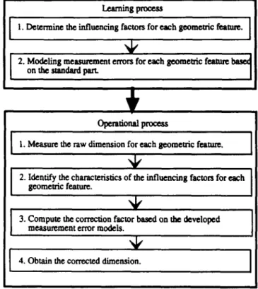
ERROR CORRECTION PROCEDURES FOR DIMENSIONAL MEASUREMENTS BY COMPUTER VISIONS Chang et al. [11] demonstrated that orientation is the major influencing factor on the measurement of the circular arc, length and angle after the image coordinate system is properly calibrated. Moreover, errors estimated from analytical models are mostly underestimated for the measurement of the radius, length and angle in laboratory experiments. There are errors due to minute shadow of parts, lighting variation and other unknown causes that cannot be easily approached analytically. In order to include all errors in the use of vision systems for error correction purposes, the empirical approach is proposed to formulate measurement correction models. This proposed framework is shown in Fig. I. The stage of determining error correction models is the "learning process," while the stage in implementing the developed models in a computer vision system is the "operational process".

For measurement correction, the following relationship should be established in the learning process:

(3)

Computer vision inspection systems 595

where ~o. is the ratio of the measured dimension to that o f its corresponding true dimension o f a geometric feature, and 0, is the orientation o f the part scanned. Then, the corrected estimate of true dimension, ~ , can be obtained in the operational process by:

/t

fr, = - - (2)

where n is the initial dimension of a geometric feature measured by a curve-fitting method.

The statistical regression method and the neural network-based method are then used to find the relationship between the geometric orientation and correction ratio. When these methods are applied, a set of input/output patterns should be obtained before the learning process. T o collect an effective set o f input/output data, one can position the rotary table within the field of view and place the part to be measured close to the center o f the rotary table. By rotating the rotary table 0 degrees in a counterclockwise (or clockwise) direction, where 0 is a predetermined increment for the part orientation, one can scan the profile of the part at different orientations. When the coordinates o f the edge points for each scanned image are obtained, the dimensions of the part can be computed. Thus, the observed dimension ratio can be obtained by

where n t is the true dimension and ~0~, 0~.

~0,, = -- (3)

/t t

is the dimension ratio of ith observation with orientation

(1) Modeling measurement errors by statistical regression

When the statistical regression method is applied to develop the required error correction models, orientation is used as an independent variable. The developed regression model will generate the

l.eaming process

1. Determine the influencing factors for catch geometric featme. [

2. Modeling measurement errors for e~h geomeCic feature base¢[

on the mmdard pan.

/

ii

Operational process

I 1. Measure the raw dimension for each geometric feature.

2. Identify the characteristics of the influencing factors for each geometric feature.

I!

3. Compute the correction factor based on the developed measurement error models.

P,

4. Obtain the corrected dimension.

Fig. I. The proposed error correction framework for the measurement of the part profile in computer vision inspection systems.

(4)

596 C. AlecChang and Chao-Ton Su

required correction ratio which is used as tp, in equation (2). The proposed error correction procedure for dimension measurement of a part can be described as follows:

Procedure 1: Error correction by Statistical Regression Models

Learning process:

Step 1. Obtain a set of observed data, (~p,,, 0~,), i = !, 2 . . . n, where tp~, is the dimension ratio of the geometric feature with the orientation of 0~, degrees;

Step 2. Determine the specific functional form to be fitted based on the observed data; Step 3. Find the regression models for observed dimension ratios and orientations for each

geometric feature by using the least squares method.

Operational process:

Step I. Measure the raw dimension, n, for each geometric feature; Step 2. Estimate the orientations of each geometric feature;

Step 3. Present the orientations of each geometric feature to the regression models and compute the estimated correction ratio, tp~;

Step 4. Obtain the corrected dimension, ~t = n/tp~, for each geometric feature.

Once the limits of the correction ratio are predicted, the prediction interval of the corrected dimension can be estimated.

(2) Modeling measurement errors by neural network

The back propagation network is used to find the relationship between tp~ and 0~, where tp, is the dimension ratio and 0~ is the orientation of the scanned feature n. In back propagation neural network, the value of the target pattern should be between 0 and 1. In addition, if the value of the input pattern is > 3, the value of the sigrnoid function will be close to I, and if the value of the input pattern is < - 3 , the value of the sigmoid function will be close to 0. Too many input patterns which have values > 3 or < - 3 will block the weight changing of the back propagation algorithm. In this study, when an architecture of neural network is defined, the orientations of each geometric feature are fed to the input layer. The output layer has several nodes, each corresponding to the dimension ratio of each geometric feature. However, the observation of the target pattern is very close to 1 (approx. 0.950--!. 120) and the observation of the input pattern is between 0 and 360. Therefore, based on the above guidelines, data sets should be scaled and shifted. In order to obtain a set of suitable training patterns to speed network learning, the observed dimension ratio is subtracted by 0.5 and its corresponding orientation is divided by 100 which would maintain the input values around 0 to 3. Once a set of training patterns are obtained and the learning rate and momentum coefficient are determined for a selected architecture, the required mapping function can be estimated. The value of the total sum of squared error for all patterns (SSE) is used as an index for the performance of the trained network. If SSE reaches a stable condition or is less than some criterion, the network training can be terminated.

Based on the discussion above, the modeling procedure by the back propagation network can be summarized as follows:

Procedure 2: Error correction by Neural Network Models

Learning process:

Step 1. Obtain a set of observed data, (tp~,, 0~, ), i = 1, 2 . . . s, where tp~, is the dimension ratio of the geometric feature with the orientation of 0~, degrees;

Step 2. Transform the observed data sets into a set of training patterns (x~, t~), i = I, 2 . . . s, where (xi, t~) = (tp~,/100, 0~, - 0.5);

Step 3. Determine the learning rate and the momentum coefficient based on the training patterns (x~, t~), i = 1, 2 . . . s;

Step 4. Choose a set of network architectures. Train each network until the difference of the SSE of two successive iterations is less than a predetermined tolerance;

(5)

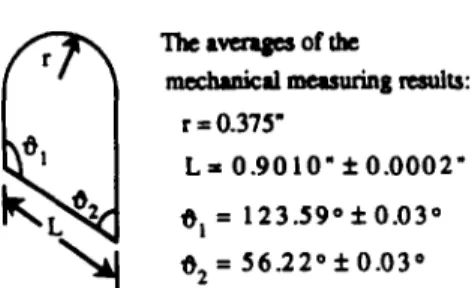
Computer vision inspection systems The avenqles of the

mechaaical m e u u t i a l l tesalts: r = 0.375"

L = 0 . 9 0 1 0 " + 0 . 0 0 0 2 " O i = 1 2 3 . 5 9 o + 0 . 0 3 ° 0 2 = 5 6 . 2 2 ° + 0 . 0 3 °

Fig. 2. A test part (material: aluminum, thickness: 0.0260" _+ 0.0005").

597

Operational process:

Step 1. Measure the raw dimension, ~, for each geometric feature; Step 2. Estimate the orientations o f each geometric feature, 0,; Step 3. Set 0" = 0~ / 100;

Step 4. Present 0~, to the trained network which is selected from Step 5 in the learning process and compute the output tp~,;

Step 5. Obtain the corrected dimension, ~t=lt/~o,, for each geometric feature, where ~o,, = ~o~, + 0.5.

IMPLEMENTATION AND VALIDATION

These two proposed procedures were implemented on the ITEX 100 Image Processing System with a personal computer connected to a camera. These experiments were carried out in a laboratory where the temperature is maintained at 20°C. T o reduce the distortion in the ITEX 100 System, the image coordinates are calibrated first. F o u r features o f a precision test part as shown in Fig. 2 are measured. Because the error correction models are part-dependent, they are fitted in the learning stage. Forty sets o f observed data for the test part in different orientations are collected. Using the proposed Procedures I and 2, the error correction models o f the test part are presented as follows:

(1) Statistical regression models

After several pilot studies, it is determined that cos 0 and sin 0 are to be used as the independent variables, where 0 is the orientation o f a geometric feature. By applying the least squares method, error correction models for the test part are built as follows:

~or = 0.963856 + 0.017924 cos 2 0r (4)

~o L = 0.9690754 + 0.005576 sin 0 L + 0.024086 cos 2 0L + 0.009085 sin 0L COS 0 L (5) ~Oa~ = 0.997877 + 0.00161 ! COS 0 L + 0.006872 COS 2 0L + 0.015025 sin 0L COS 0 L (6) tOa2 = 1.002895 -- 0.005887 sin 0L -- 0.014004 COS: 0L -- 0.023232 sin 0L COS 0L (7) where ~0,, ~0L, ~Oal, and ~oa~ are the ratios o f radius, length, angle l and angle 2, respectively. 0, is the orientation of the circular arc and 0L is the orientation o f the straight line edge, angle ! and angle 2. Note that a same orientation can be specified for all adjoining geometric features.

(2) Neural network-based models

These four geometric features on the sample part associate with one of the two orientation angles. Therefore a neural network can be structured with two input patterns and four target patterns. Thus ( 0 r / 1 0 0 , 0 L / 1 0 0 ) t is used for the input layer and (tp, - 0.5, tOE -- 0.5, ~OS, -- 0.5, tO.9: -- 0.5) t is used for the output layer. The Parallel Distributed Processing Software (PDP) with a back propagation learning algorithm is used for the network training [27].

Through several pilot runs, the learning rate and the momentum coefficient are set at 0.20 and 0.90 from a pilot study. Several different network's architectures have been tried. Results of network 2 - 3 - 3 - 4 as shown in Fig. 3 demonstrates the best performance. Accordingly, the model

(6)

5 9 8 C . A l e c Chang and Chao-Ton S u

input output

layer hidden layer layer

q~- 0.5

100 q~t.- 0.5

01'

100 q~o t - 0.5

% -

0.5

F i g . 3. The architecture of network 2 - 3 - 3 - 4 .

of network 2 - 3 - 3 - 4 is chosen to estimate the required correction ratios when a new input pattern (0,/100, 0L/100)' of an incoming part is given.

The neural network-based correction models for the ratios of radius, length, angle 1 and angle 2 of the test part are summarized as follows:

~Pr = 0.5 + [I + exp( -net~,)l-~ (8)

~PL = 0.5 + [1 + exp( -- netp9)]-a (9)

~Po, = 0.5 + [I + exp(-- netp~0)] -~ (10)

~Pa2 = 0.5 + [1 + exp(--netp. )]-~ (11)

where netp,=

Zjw~japj+ b~.j

belongs to previous layer based on network 2 - 3 - 3 - 4 (Fig. 3), apo = 0,/100 and ap~ = 0L/100 for

api=

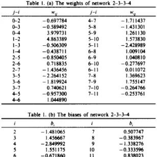
(1 + exp(--netp,)) -~ (i = 2, 3 . . . 11). 0, is the orientation of the circular arc and 0L is the orientation of the straight line edge, angle I and angle 2. The weights and biases of this network model, w~j and b,, are listed in Table 1.

(3) A

comparison

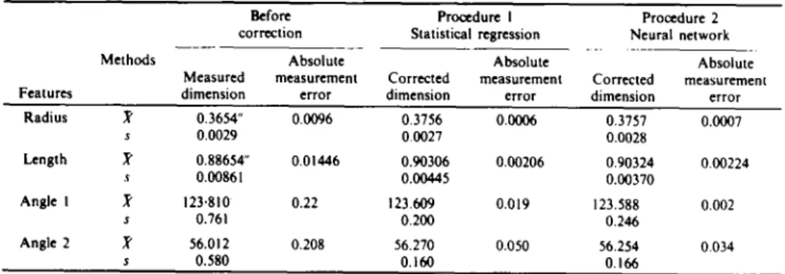
To compare performances of these two error correction procedures, the test part is scanned another 20 times so that an additional 20 sets of edge points are obtained in different orientations. The orientations of these 20 scans are listed in Table 2. A statistical summary of the implementation results from the error correction by using procedure 1 and procedure 2 is shown in Table 3. Compared to their true dimensions, the absolute measurement errors are also listed correspondingly.

Table I. ( a) The weights of network 2 - 3 - 3 - 4

j - i W',l j - i w,i 0 - 2 - 0 . 6 9 7 7 8 4 4 - 7 - 1 . 7 1 1 4 3 7 0 - 3 - 0 . 5 8 9 4 9 2 5 - 8 - 1.431301 0 - 4 3 . 9 7 9 7 3 1 5 - 9 1 . 2 6 1 1 3 0 I - 2 4 . 8 6 3 3 8 9 5 - 1 0 1 . 5 7 3 8 3 0 I -3 - 0. 5 0 6 3 0 9 5 - I 1 - 2 . 4 2 8 9 8 9 I - 4 - 0 . 4 3 8 7 1 1 6 - 8 1 . 0 0 9 1 0 4 2 - 5 - 0 . 8 5 0 4 0 5 6 - 9 1 . 0 4 0 8 1 0 2~b 0 . 7 1 8 8 3 5 6 - 1 0 - 0 . 2 7 7 6 9 7 2 - 7 - 1 . 4 3 6 4 5 6 6--11 0 . 0 1 1 0 7 2 3 - 5 - 2 . 2 6 4 1 5 2 7 - 8 1 . 3 6 9 6 2 3 3~b - 1 . 8 1 9 9 2 4 7 - 9 1 . 7 5 5 1 4 7 3 - 7 0 . 7 4 0 6 2 1 7 - 1 0 - 0 . 2 6 4 7 6 6 4 - 5 - 0 . 9 5 7 3 0 0 7 - 1 1 - 0 . 2 5 3 7 6 I 4 - 6 1 . 0 4 4 8 9 0

Table 1. (b) The biases of network 2 - 3 - 3 - 4

i b, i b, 2 - 1 . 4 8 1 0 6 5 7 0 . 5 0 7 7 4 7 3 1 . 4 5 6 6 6 7 8 - 0 . 3 8 3 9 6 7 4 - 2 . 8 4 9 9 9 2 9 - 1 . 3 3 8 2 7 6 5 1 . 5 5 1 1 7 5 10 - 0 . 3 3 3 5 9 6 6 - 0 . 6 7 1 8 6 0 I I 0 . 8 3 8 0 2 3

(7)

C o m p u t e r vision inspection systems

Table 2. Twenty different orientations of the test part

No. 0, 0 t No. 0, 0t I 16.7499 162.7700 II 186.4145 332.8866 2 46.7057 192.1600 12 211.9046 357.6542 3 51.7330 197.1156 13 226.9896 12.2848 4 56.6248 202.1813 14 236.9372 22.3381 5 66.3256 212.0437 15 256.6371 41.9351 6 86.1563 232.1433 16 261.8560 46.9985 7 121.0246 267.5440 17 316.1019 102.5291 8 136.0842 282.9632 18 326.1614 112.6399 9 141.0935 287.9212 19 336.2495 122.7072 10 145.9828 292.6986 20 346.1750 132.6138

Note: 0, is the orientation of the circular arc and 0 t is the orientation of the straight line edge, angle I and angle 2.

599

A statistical test is conducted to decide whether the absolute measurement errors from the neural network-based method are different from those using the statistical regression method. This is to test the hypothesis

H0: #N =#R.,

ne{r,L,~l,~2}

against the alternative

Ha : /~, #: #R,

where N, and R~ denote the absolute measurement error using the neural network-based method and the statistical regression method for each geometric feature, respectively./~N, and/zR, are the means of N~ and R,, respectively. Since the distribution of absolute measurement errors passed a normality test, the following t distribution is applied

t* ~,~, -- ~'n, (s 2, + s 2, )2 (n - 1) (12)

2 ~ ' sN, + s~,

n

where ~'N., ~'s,, and s~,,2 s 2 are simple means and variances, n is the sample size and v is the degree of freedom for which a round-off integer is used.

For the radius measurement,

0.0007 - 0.0006

t * = =0.115, v = 3 8 .

k/0.00272 + 0.00282 20

Although the error correction model for the radius measurement based on the statistical regression method performs better, this result is not statistically significant with ct = 0 . 0 5 level [t(0.975, 3 8 ) = 2.025]. Thus, the hypothesis of Ha is injected, i.e. #s, is not different from #R, statistically. Therefore, we conclude that the error correction results of radius for procedure 1 (statistical regression models) and procedure 2 (neural network-based models) are not significantly

Table 3. The statistical summary of corrected dimensional measurements

Features

Methods

Before Procedure I

correction Statistical regression

Absolute Absolute

Measured measurement Corrected measurement

dimension error dimension error

Procedure 2 Neural network Absolute Corrected measurement dimension error Radius ~" 0.3654" 0.0096 0.3756 0.0006 0.3757 0.0007 s 0.0029 0.0027 0.0028 Length ~" 0.88654" 0.01446 0.90306 0.00206 0.90324 0.00224 s 0.00861 0.00445 0.00370 Angle I ~" 123.810 0.22 123.609 0.019 123.588 0.002 s 0.761 0.200 0.246 Angle 2 ~" 56.012 0.208 56.270 0.050 56.254 0.034 s 0.580 0.160 0.166

(8)

600 C. Alec Chang and Chao-Ton Su

Table 4. t* values between absolute errors from the neural network-bued method and the statistical regression method

Feature Radius Length Angle ! Angle 2

t* 0.115 -0.139 - 0.240 -0.362

t,*,,,~ t(0.975, 38) = 2.025 t(0.025, 34) = -2.034 t (0.975, 37) = 2.027 t (0.975, 38) = 2.025 Note: t* values are used to test whether the absolute measurement errors of the neural network-based method are different

from those of the statistical regression method.

different. Calculated t* values to test the absolute measurement errors of the neural network based models and the statistical regression based models for error correction are listed in Table 4. It is also concluded that the measurement results of length and angle for procedures 1 and 2 are not significantly different.

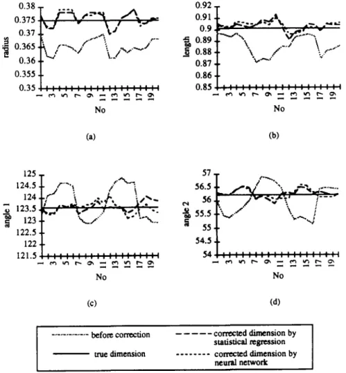
Dimensional measurements with respect to part orientation before and after error correction by these two methods are shown in Fig. 4. Both error correction results using regression models and neural network models demonstrate a very good performance for corrected dimensional measurements using computer visions.

D I S C U S S I O N

When the statistical regression method is used, the specific functional form must be specified in advance. In this study, the sine and cosine transformations on O (orientation) are used for regression relation between radius ratio, length ratio, angle ratio and orientations. In general, the form of the fitting function should be chosen carefully when the statistical regression method is applied. For

0.38 0.375 0.37 ~ 0.365 0.36 0.355 0.35 0.92 , j - : : - ~ # , . - . ~ , . , , A - - 0.91 ? j .,

..,.~,j

% . r 0.9 ; - "

-

~ 0.89.

L:-'-.I ,,/,.--"

o 0 . 8 7 , 0.86, J_ _t _~ ;,_ ,_ ,_ ,_ , , , , :: : ..: ,.,. 0 . 8 5 I I U g I g I I J V l I I I B I I I I ~ ~ r ~ ~ ~ ee~ ~'~ r'~ N o (a) ,.~---_.~-"4- t~, . - \ / " : : : : : : : : : : : : : ' : : : ! N o (b) 125, 124.5, 124, _~ 123.5, 123. 122.5, 122 121.5

/

--,~ / ' ~ " ~ , ~ . . j . . . .. I : : : : : : : : : : : : : , : : : : N o (c) 57 56.5 56 t'q 55.5 g 55 54.5 54 I 1 : : : : : : : : : : : : : : : : : : N o (d) ... before correction true dimension . . . corrected dimension by statistical regression . . . corrected dimension by neural network Fig. 4. Measurement results for the test part.

(9)

Computer vision inspection systems Table 5. Total sum of squared errors of six networks

Network epoch SSE

2-4-4 35,500 0.00165 2--6-4 24,000 0.00151 2-8--4 38,500 0.00145 2-2-2--4 30,000 0.00360 2-3-3-4 30,000 0.00140 2 ~ ~ A 31,500 0.00176

Note: the back propagation procedure is said to he operated one epoch when the forward and backward passes are swept through the whole training patterns one time.

601

example, if one of the following simple models is selected for the radius measurement instead of using equation (4):

~Pr = 0.973765 - 0.0001520r (13)

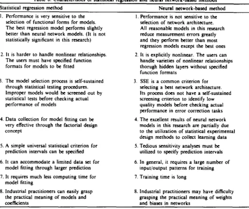
cpr = 0.973321 + 0.000556 COS 0r -- 0.000257 sin 0r (14) where 0r is the orientation (measured in radians) based on the center, its performance to reduce measurement errors is not satisfactory. Fortunately, a required testing process in the statistical regression method will reject both models by a common criterion of a = 0.05 for F values. The probability values of F (PROB > F) for equations (13) and (14) are 0.8207 and 0.9341, respectively. This statistical testing and screening process usually leads to acceptable models with satisfactory performances. As long as the form of the fitting function is determined properly, the statistical regression method can effectively find the mapping coefficients. From Table 4, one can see that the statistical regression models from equations (4) to (7) perform slightly better. This is due to a very careful selection of these equation formats by observing error patterns from initial measurements. A principal strength of the neural network approach over the statistical regression method is that the neural network is explicitly nonlinear through hidden layers. It is a more general mapping procedure that a specific function format is not required in model building. Moreover, the performance is not sensitive to different network's architectures in this study. The performances of six different networks are listed in Table 5. Among them, network 2-3-3-4 has the smallest SSE and network 2-2-2-4 has the largest SSE. In this study, each of the six trained networks gives improved measurement results. That is to say, the neural network-based method will give satisfactory results for the error correction of dimensional measurements in general. But SSE cannot be directly linked with performance of network models. There are no uniform screening processes for network models before they are actually implemented. A performance checking is required before a model can be adopted as the error correction model in inspection processes. A possible drawback of the neural network approach is that is usually requires many training data and tremendous numbers of iterations to complete learning. The building of the neural network-based models in this study takes advantage of the factorial design concept. These data are collected by rotating the sample part with a constant incremental angle. Although the use of a factorial design concept for data collection is not necessary, the amount of training data required for building good network models will be greatly reduced. Moreover, the influencing factors in this study have been selected by the statistical method (ANOVA) for model fitting. Thus, the input variables for neural network training have been reduced to one influencing factor [I 1]. Another major difference is that the confidence intervals of estimated coefficients and responses from models can be specified for the statistical regression method based on statistical variations. The neural network-based method has to utilize a tedious sensitivity analysis for this task. The different characteristics of the statistical regression method and the neural network-based method for modeling measurement errors are summarized in Table 6.

C O N C L U S I O N

With the advent of computer vision inspection, a proper error correction of dimensional measurements is essential. Two error correction procedures using the statistical regression and the neural network-based methods for dimensional measurements in computer vision systems are

(10)

602 C. Alec C h a n g and C h a o - T o n Su

Table 6. Characteristics of statistical regression and neural network-based methods

Statistical regression method Neural network-based method

l. Performance is very sensitive to the selection of functional forms for models. The best regression model performs slightly better than neural network models. (It is not statistically significant in this research) 2. It is harder to handle nonlinear relationships.

The users must have specified function formats for models to be fitted

3. The model selection process is self-sustained through statistical testing procedures. Improper models would be screened out by statistical tests before checking actual performance of models

4. Data collection for model fitting can be very effective through the factorial design concept

5. A simple universal statistical criterion for prediction intervals can be specified 6. It can accommodate a limited data set for

model fitting through larger prediction 7. It requires much less computing time for

model fitting

8. Industrial practitioners can easily grasp the practical meaning of models and coefficients

I. Performance is not sensitive to the selection of network architecture. All reasonable models in this research

reduce measurement errors greatly and they perform better than most regression models except the best ones 2. It is explicitly nonlinear. The users can

handle varieties of nonlinear relationships thorugh hidden layers without specified function formats

3. SSE is a common criterion for selecting a best network architecture. Its process does not have a self-sustained screening criterion to identify low quality models before checking actual performance in error correction tasks 4. The excellent results of neural network

models in this research are partially due to the utilization of statistical experimental design methods to collect learning data 5. Tedious sensitivity analyses must be

utilized to specify prediction intervals 6. In general, it requires a large number of

input/output patterns for training 7. Training time is long

8. Industrial practitioners may have difficulty grasping the practical meaning of weights and biases in networks

implemented and compared in this paper. Experimental results show that both of these two procedures can be used for the purpose of correcting measurement errors. These two proposed procedures for modeling measurement errors can assist quality control practitioners utilizing computer vision systems for measurement and inspection tasks. Both of these procedures are applicable to different geometric features, such as the correction of estimated vertex of the parabola, foci of ellipse, and loci and vertices of hyperbola. They should be also applicable to correct the estimation of coefficients for curves with higher degrees.

In order to adopt the regression method effectively, the form of the fitting function should be defined in advance, i.e. the specific form of a correction function must be chosen first and then a fitting is carried out according to the minimal sum of square errors. On the other hand, if the form of the fitting function cannot be specified, then the neural network-based method is suggested. When the learning rate, momentum coefficient and number of nodes in the hidden layers are carefully chosen, the back propagation network does not require any a priori information and can map the input patterns to the output patterns properly.

R E F E R E N C E S

I. A. A. Rodriguez, ,I. R. Mandeville and F. Y. Wu. System calibration and part alignment for inspection o f 2 D electronic circuit patterns. SPIE 1332, Optical Testing and Metrology lIi: Recent Advances in Industrial Optical Inspection, pp. 25-35 (1990).

2. A. W. Burner, W. L. Snow, M. R. Shortis and W. K. G o a d . L a b o r a t o r y calibration and characterization of video cameras. SPIE 1395, Close-Range Photogrammetry Meets Machine Vision, pp. 664-671 (1990).

3. Y. R. Shiau and B. C. Jiang. Determine a vision system's 3D coordinate m e a s u r e m e n t capability using taguchi methods. Int. J. Prod. Res. 29, 1101-1122 (1991).

4. L. L. W a n g and W. H. Tsai. C a m e r a calibration by vanishing lines for 3-D c o m p u t e r visions. IEEE Trans. Pattern Anal. Mach. lntell. 13, 370-376 (1991).

5. R. M o h r and E. Arbogast. It can be done w i t h o u t c a m e r a calibration. Pattern Recogn. Lett. 12, 39-43 (1991). 6. Z. C. Lai. The calibration of a stereo vision system with two camera. 1992 IPPR Conference on Computer Vision.

Graphics and Image Processing, Taiwan, pp. 41-48 (1992).

7. G. G. Wagner. Vision m e t h o d o l o g y as it applies to industrial inspection applications. Gauging: Practical Design and Application, pp. 410-418. Society o f M a n u f a c t u r i n g Engineers (SME) (1983).

(11)

Computer vision inspection systems 603

9. F. Etesami and J. J. Uicker. Automatic dimensional inspection of machine part cross sections using Fourier analysis.

Computer Vision Graph. Image Process. 29, 216-247 (1985).

10. C. A. Chang, L. H. Chen and J. 1. Ker. Et~cient measurement procedures for compound part profile by computer vision.

Computers Ind. Engng 21, 375-377 (1991).

11. C. A. Chang, L. G. David, L. H. Chen and C. T. Su. Error correction models for measurement and inspections in computer vision systems. 2nd Industrial Engineering Research Conference Proceedings, pp. 629-633 (1993).

12. G..I. Udo, Neural networks applications in manufacturing process. Computers Ind. Engng 23, 97-100 (1992).

13. K. Sasaki, D. Casasent and S. Natarajan. Neural net selection of features for defect inspection. Proc. SPIE Int. Soc. Opt. Engng. 1384, 228-233 (1991).

14. M. A. Javed and S. A. C. Sanders. Neural networks based learning and adaptive control for manufacturing systems.

Proceedings of the IEEE/RSJ International Workshop on Intelligent Robots and Systems-lROS '91, pp. 242-246. IEEE

Service Center, Piscataway, NJ (1992).

15. C. Neubauer. Fast detection and classification of defects on treated metal surfaces using a backpropagation neural network. 1991 IEEE International Joint Conference on Neural Networks, pp. 1148-1153. IEEE Service Center,

Piscataway, NJ (1991).

16. J. R. Kroh, T. S. Durrani and R. Chapman. Neural network architecture for circular features extraction in binary patterns. Electron. Lett. 27, 1879-1880 (1991).

17. O. Masory. Monitoring machining processes using multi-sensor readings fused by artificial neural network. J. Mater. Process. Technol. 28, 231-240 (1991).

18. T. H. Hou, L. Lin and P. D. Scott. A neural network based automated inspection system with an application to surface mount devices. Int. J. Prod. Res. 31, 1171-1187 (1993).

19. J. I. Ker, M. Lynch and A. Kalale. A neural network approach to machine vision based radius inspection, intell. Engng Syst. ,4rtif. Neural Networks 2, 541-546 (1992).

20. H. B. Hwarng and N. F. Hubele. Back-propagation pattern recognition for ~" control charts: methodology and performance. Computers ind. Engng 24, 219-235 (1993).

21. F. Y. Wu. Applications of neural network in regression analysis. Computers ind. Engng 23, 93-95 (1992).

22. J. W. Ball and P. C. Jurs. Automated selection of regression models using neural networks for ~3C NMR spectral predictions. Analyt. Chem. 64, 379-386 (1993).

23. T. R. Holcomb and M. Morari. PLS/neural networks. Computers chem. Engng 16, 393-411 (1992).

24. B. Joseph, F. H. Wang and D. S. Shieh. Exploratory data analysis: a comparison of statistical methods with artificial neural networks. Computers chem. Engng 16, 413-423 (1992).

25. C. A. Chang and K.-H. Hsieh. Object identification and profile inspection by computer vision systems in multiple objects scenario. Proceedings the Third Industrial Engineering Research Conference, Atlanta, pp. 503-508 (1994).

26. C. A. Chang. Precision measurement and automated inspection for part profile by computer vision and CMM.

Proceedings, 13th Modern Engineering and Technology Seminar, Taipei, Vol. 6, pp. 59-75 (1990).

27. J. L. McClelland and D. E. Rumelhart. Explorations in Parallel Distributed Processing. M1T Press, Cambridge, MA