有限元素生物力學分析:表面網格最佳化及納氏漏斗胸手術之力學分析

國 立 交 通 大 學

機 械 工 程 學 系

博 士 論 文

有限元素生物力學分析:表面網格最佳化及

納氏漏斗胸手術之力學分析

Finite element biomechanical analysis: surface mesh optimization

and analysis for Nuss pectus excavatum repair

研 究 生: 徐振予

指導教授: 陳大潘 教授

有限元素生物力學分析:表面網格最佳化及

納氏漏斗胸手術之力學分析

研究生:徐振予 指導教授:陳大潘 教授

摘 要

本論文之目的，在於研究有限元素法於生物力學分析上之應用，研究內容包括了表 面網格最佳化以及納氏漏斗胸手術之生物力學分析。對於生物力學分析研究而言，建立 一個合適之有限元素網格，是一個非常重要的步驟，其中又以表面網格的建立最為重 要，一般而言，表面網格乃建立於預先定義之模型表面上，但對於大部分之生物力學分 析研究而言，其分析模型通常經由量測或斷層掃描資料建立而成，因此無法利用數學模 式完整定義整個模型表面，例如脛骨、脊椎以及胸腔模型等研究，為了改善上述分析模 型之表面網格品質，我們提出了一套表面網格最佳化方法，其中包括了三角形網格與四 邊形網格之轉換、C1 連續之表面方程式建立，以及微基因演算法表面網格平滑化處理， 本方法可應用於模型表面網格之最佳化，而不需預先提供模型之表面方程式，因此可適 用於生物力學分析模型之應用。 漏斗胸是一項常見的先天性胸廓畸形，其病症為患者之胸骨，以及肋軟骨向患者體 內凹陷，而於患者前胸形成漏斗狀之變形。納氏手術為目前常用之漏斗胸微創手術，它 的手術方式為，將矯形金屬板植入於漏斗胸患者之胸骨凹陷處，將患者前胸之凹陷處頂 高，以達到矯正之目的。在手術過程當中，患者之胸廓會隨著胸骨之頂高而變形，然而， 經由該變形所引發之應力，也同時產生並作用於患者胸腔骨骼上。在本論文中，我們利 用半自動化方式，建立了五個漏斗胸患者之胸腔模型，並分析它們在經過納氏手術矯正 之後，患者胸腔骨架上之應力與應變之分佈情形。根據分析結果發現，患者於手術後， 其背部靠近脊椎附近，有大量的應力產生，其中大多集中在第三到第七對肋骨上，這個 現象可用來解釋，某些漏斗胸病患，於納氏手術後產生背痛之原因，並且可能與少部分 患者，於手術後發生脊柱側彎之原因有關。此外，我們利用有限元素分析結果，建立兩 套肺容積估測方法，藉由量測患者胸腔容積之變化，可用來估測肺容積之變化，根據量 測結果發現，這五位患者之胸腔容積，分別增加了 2.72%到 8.88%不等的容積。

Finite element biomechanical analysis: surface mesh optimization

and analysis for Nuss pectus excavatum repair

Student: Zhen-Yu Hsu Advisor: Da-Pan Chen

Abstract

The purposes of this thesis are focused on the finite element biomechanical analysis, which contains surface mesh optimization and biomechanical analysis of Nuss pectus excavatum repair. For a biomechanical research, one of the significant problems is to create an appropriate finite element volume mesh and the surface mesh generation plays a crucial role in finite element volume mesh generation. Usually surface meshing methods in three dimensions generate meshes relying on prescribed patch interpolation. For some biomechanical researches, the analyzed models, which were usually reconstructed based on measured data or computer tomography scan data, do not have well defined surface function, such as tibia, spine and rib cage models. In order to improve the surface mesh quality of the reconstructed geometrical models, an approach of surface meshing optimization procedure is developed, which consists of a conversion scheme for primary triangular and quadrilateral

surface meshes, a C1 continuous surface function reconstruction and a micro-genetic

algorithm (MGA) mesh smoothing procedure. This procedure performs surface mesh optimization without pre-defined surface function. The practical cases are given to demonstrate its successful performance and its versatility.

Pectus excavatum (PE) is one of the commonly found congenital chest wall deformity. It is characterized by depression of the sternum and the lower costal cartilages, producing a concave appearance to the anterior chest wall. The Nuss procedure is a minimal invasion technique that corrects pectus excavatum by inserting a pre-bent bar under the depressed sternum to elevate the sternum. After the Nuss procedure, the chest wall is deformed with the raised sternum and a reasonable amount of stress is induced on the chest wall. In this thesis, five patient-specific finite element models were generated to analyze the stress and the strain distributions induced on the chest wall after the Nuss procedure. The finite element models were reconstructed by applying a semiautomatic procedure based on patients’ computer tomography slices. The simulation results show that there are greater stresses occurred over the back and concentrated on the third through seventh ribs bilaterally, near the vertebral

column. These phenomena might explain back pain on some patients after insertion of pectus bar and sporadically reported thoracic scoliosis after Nuss procedure. Moreover, we

developed two thoracic volume measurement procedures to estimate the thoracic volume change of postoperative PE patients. The thoracic volume measurement procedure was performed based on the finite element analysis results and the increase of lung volume is estimated by measuring the increase of thoracic volume. The estimated results shown that the thoracic volume is increased about 2.72% to 8.88%.

致謝

在此首先要感謝我的指導老師陳大潘教授，在交大這段不算短的日子裡，承蒙老師 辛勤的指導，讓我得以順利完成博士學位；在這段求學期間當中，我所學習到的除了專 業知識上的進步之外，還有從事研究工作該有的態度與方法，這些成果對於我將來就業 以及為人處世上，都將會有莫大的助益，在此深深的感謝老師給我的一切幫助。此外要 特別感謝的人，就是高速電腦中心的林芳邦老師，在林老師的共同指導下，我完成了我 的第一篇論文，並且在老師的介紹下，認識了我的太太喬媜，真的是十分的感謝林老師。 另外要感謝工研院廖俊仁博士以及林口長庚兒童醫院的張北葉主任，有幸得與你們這些 先進們合作，讓我獲得了非常寶貴的跨領域合作經驗，這些經驗都是非常難得且重要 的，謝謝你們。 在交大就學的這段期間，感謝父母以及家人的支持，讓我得以持續我的求學之路； 此外，我的太太喬媜以及女兒千媃，謝謝你們這段時間對我的幫助與寬容，讓我得以專 心於課業上，你們的支持是我最大的幸福。感謝高速電腦中心吃飯班成員昀德、哲男等 人，謝謝你們陪我經歷這段不算短的求學階段。最後要感謝研究室的立傑學長、達人、 信賢、建弘以及歷屆的學弟們，能認識你們是緣分也是我的福氣，謝謝大家。

Table of contents 摘要………Ⅰ Abstract………Ⅱ 致謝………Ⅳ Table of contents………Ⅴ List of tables………Ⅶ List of figures………Ⅷ Chapter 1 Introduction………1 1.1 Overview………1

1.2 Surface mesh optimization………1

1.3 Pectus excavatum………3

Chapter 2 Genetic algorithm………8

2.1 Genetic algorithm………8 2.1.1 Cording………8 2.1.2 Initialization………9 2.1.3 Selection………9 2.1.4 Crossover………10 2.1.5 Mutation………10 2.2 Micro-genetic algorithm………11

Chapter 3 Surface function reconstruction………16

3.1 Gradient estimation………16

3.2 Interpolation method………17

3.3 Geometrical accuracy comparison………20

Chapter 4 Surface mesh smoothing………27

4.1 Mesh generation………27

4.1.1 Triangular mesh generation………27

4.1.2 Quadrilateral mesh generation………27

4.1.3 Mesh structure modification operators………28

4.2 Micro-genetic algorithm surface mesh smoothing………29

4.2.2 Fitness function………30

4.3 Surface mesh smoothing results………32

Chapter 5 Pectus excavatum repairs………49

5.1 Pectus excavatum repairs………49

5.2 Nuss procedure………49

Chapter 6 Finite element biomechanical analysis and thoracic volume measurement…54 6.1 Patient-specific finite element models………54

6.2 Finite element analysis………55

6.3 Thoracic volume measurement………56

6.3.1 Method 1: intersection method………56

6.3.2 Method 2: surface approximation method………57

6.4 Results………60

6.4.1 Finite element analysis results………60

6.4.2 Thoracic volume measurement results………62

Chapter 7 Conclusions………84

References………86

List of tables

Table 3-1 Surface errors of the test functions for C0 and C1 surface reconstruction…………26

Table 4-1 The comparison between conjugate gradient method and MGA method using the saddle geometry………38

Table 4-2 Mesh quality improvement for the triangular surface meshes………38

Table 4-3 Mesh quality improvement for the quadrilateral surface meshes………38

Table 6-1 Five pectus excavatum patients information………64

List of figures

Fig. 1-1 A 7-year-old boy with pectus excavatum………6

Fig. 1-2 Pectus index………7

Fig. 2-1 Flowchart of the traditional genetic algorithm………12

Fig. 2-2 Roulette wheel selection………13

Fig. 2-3 Tournament selection………13

Fig. 2-4 Crossover (a) one point crossover (b) two point crossover………14

Fig. 2-5 Mutation………14

Fig. 2-6 Flowchart of the micro-genetic algorithm………15

Fig. 3-1 Triangles in the triangulation………21

Fig. 3-2 Node V on the boundary………21

Fig. 3-3 Notation of a triangle………22

Fig. 3-4 Thirty-six points and triangulations………22

Fig. 3-5 (a) test function 1 (b) test function 2………23

Fig. 3-6 Surface errors of test function 1 (a) C0 surface (b) C1 surface………24

Fig. 3-7 Surface errors of test function 2 (a) C0 surface (b) C1 surface………25

Fig. 4-1 Edge swapping (a) triangular elements (b) quadrilateral elements………36

Fig. 4-2 Node eliminating (a) triangular elements (b) quadrilateral elements………36

Fig. 4-3 Edge dividing (a) triangular elements (b) quadrilateral elements………37

Fig. 4-4 Design parameters definition on a triangle………37

Fig. 4-5 Triangular surface mesh of saddle (a) Original surface mesh (b) Surface mesh after MGA smoothing (c) Surface mesh after conjugate gradient smoothing…39 Fig. 4-6 Quadrilateral surface mesh of saddle (a) Original surface mesh (b) Surface mesh after MGA smoothing (c) Surface mesh after conjugate gradient smoothing………40

Fig. 4-7 Triangular surface mesh of wing-fuselage (a) Original surface mesh (b) Surface Mesh after smoothing………41

Fig. 4-8 Quadrilateral surface mesh of wing-fuselage (a) Original surface mesh (b) Surface mesh after smoothing………42

Fig. 4-9 Triangular surface mesh of foot (a) Original surface mesh (b) Surface mesh after smoothing………43

Fig. 4-10 Quadrilateral surface mesh of foot (a) Original surface mesh (b) Surface mesh after

smoothing………44

Fig. 4-11 Triangular surface mesh of rat (a) Original surface mesh (b) Surface mesh after smoothing (c) Original surface mesh (enlarged) (d) Surface mesh after smoothing (enlarged)………46

Fig. 4-12 Quadrilateral surface mesh of rat (a) Original surface mesh (b) Surface mesh after smoothing (c) Original surface mesh (enlarged) (d) Surface mesh after smoothing (enlarged)………48

Fig. 5-1 A transverse inframammary incision with upward curvature was made midway between the nipples, and a short vertical extension in the midline was made to expose the superior sternum [65]………51

Fig. 5-2 A thin stainless-steel bar was placed under the sternum to elevate the sternum and attached to the appropriate rib on each side with fine wire [65]………52

Fig. 5-3 The pectus bar is pre-bent to match a desired shape [66]………52

Fig. 5-4 Nuss procedure [25] ………53

Fig. 5-5 Pectus bar is secured to ribs with a stabilizer plate [67]………53

Fig. 6-1 Segment on AMIRE (a) automatic segments (b) modified segments………65

Fig. 6-2 Convergence test………66

Fig. 6-3 Reaction forces applied to a pectus bar………67

Fig. 6-4 Boundary conditions of a FEA model………67

Fig. 6-5 Major internal structures of human [71] ………68

Fig. 6-6 Cutting plane………69

Fig. 6-7 Segment of intratoracic volume (a) original (b) deformed………70

Fig. 6-8 Original cyclinder………71

Fig. 6-9 Flow chart of surface approximation procedure………72

Fig. 6-10 Singular key-point identification………73

Fig. 6-11 (a) Skinny surface with 26×28 patches (b) 6×12 patches26×28 patches…………74

Fig. 6-12 Approximated surface consisted of 16×16 Ferguson’s bicubic patches (a) without smoothing (b) smoothing………75

Fig. 6-13 Volume calculation of a pyramid………76 Fig. 6-14 The relationship between elevating force and the displacement of the end of sternum

………76

Fig. 6-15 Deformation with different elevating force (patient one)………77

Fig. 6-16 Stress distribution of patient one with an elevating force 140N………77

Fig. 6-17 Strain distribution of patient one with an elevating force 140N………78

Fig. 6-18 Variation of strain of patient one along the right fifth costal cartilage and rib with an elevating force 140N………78

Fig. 6-19 Intrathoracic volume (a) original (b) after Nuss procedure………79

Fig. 6-20 The relationship between elevating force and the increasing volume of intrathoracic ………80

Fig. 6-21 (a) rib cage model of pre-operative PE patient (b) approximated surface (c) thoracic volume measurement(1885.809cm3) ………81

Fig. 6-22 (a) rib cage model of postoperative PE patient (b) approximated surface (c) thoracic volume measurement(2129.294cm3) ………83

Chapter 1.

Introduction

1.1 Overview

Finite element analysis (FEA) is a popular numerical method which is widely used in science and engineering. In a finite element biomechanical analysis, the structural system is first modeled by a set of appropriate subdivisions called elements and then calculated with assigned material properties and applied boundary conditions. The FEA provides a convenient way to investigate the biological phenomena of an object without practical experiment. In this thesis, we employ the finite element analysis to perform the biomechanical analysis of pectus excavatum (PE) patients after a Nuss procedure.

It is well known that a quality mesh is imperative to enhance the accuracy of a finite element simulation. In engineering practice, meshes can be generated on the boundary and/or in the interior of the object, which correspond to surface meshing and volume meshing, respectively. Usually, a well defined geometrical model is requested before the mesh generation. The geometrical model can be defined with algebraic form or defined by patches. However, for some biomechanical researches, the geometrical models were reconstructed from measuring data or computer tomography (CT) scan data [1,2], and it was difficult to provide a pre-defined surface function. In this thesis, we present a different approach that surface meshing is on a set of unorganized points in which the surface function is yet to be defined [3].

1.2 Surface mesh optimization

For surface meshing, most existing methods [4] generate the surface mesh based on pre-defined surface functions, either in parametric patches or in algebraic form, by using existing mesh generation schemes such as Delaunay Triangulation [5] or Advancing Front

Methods [6].However, in many real cases, the given data may just be a set of unorganized

points, in which its surface function cannot be devised in a usual fashion. It is often encountered in the applications of biomechanics, which require a geometrical reconstruction from a set of sampling points that is extracted from a sequence of scanned images, e.g. histological sections in tomography. An immediate way to generate a surface mesh for this application is to triangulate the given points [7-10]. However, some sets of such sampling

points can be scattered and irregular, and results in locally ill-posed meshes, which may not acceptable for finite element analysis. In this study, a posteriori approach is adopted to tackle this problem: The given points are first triangulated to generate a triangular mesh and/or convert to the quadrilateral mesh and then an additional procedure is introduced to enhance the quality of the mesh. For finite element meshes, the common used procedure for this enhancement is mesh smoothing.

The most popular mesh smoothing method is Laplacian smoothing [11], in which every internal grid node is repositioned at the geometrical center of the adjacent nodes. Generally, for surface mesh smoothing, Laplacian smoothing is first employed on a parametric plane and then maps the result onto the physical surface domain. It is well known that the mapping between a reconstructed surface and its parametric plane for Laplacian smoothing strongly affects the resultant mesh quality. A given unorganized point set is usually lack of geometrical regularity in distribution. It cannot guarantee to form a proper primary mesh for the mapping of the Laplacian smoothing.

Optimization-based mesh smoothing technique is another way to smooth the finite element mesh, in which the new location of node is found by using the optimization algorithms [12-15]. Freitag [12] presented several articles described about the finite element mesh smoothing techniques, which contained smart Laplacian smoothing, optimization-based smoothing and the combination of both, in two-dimensional plane mesh and three-dimensional tetrahedral mesh. For the combination method, the smart Laplacian smoothing is used to adjust every internal node and is followed by the optimization-based algorithm, the steepest decent method [16], in only the poorest-quality elements [12]. The steepest decent method searches an optimal solution by a given initial step along a search direction, which is calculated from the gradients of the object function, i.e. mesh quality measurement. However, the calculating of gradients according to the real coordinates is inconvenient for this application, in which the surface function is yet to be defined. Besides, the search direction may let the nodes to deviate from the original surface.

Garimella et al. [14] presented a surface mesh quality optimization procedure that the nodes are repositioned based on element-based local parametric spaces. They employ the conjugate gradient method [16], whose search direction is estimated by computing the gradients of the mesh quality measurement with respect to the local parametric spaces, to reposition the nodes to enhance the mesh quality. It is beneficial that mesh smoothing based on local parametric spaces can remain the nodes close to the original surface. The calculation of the gradients of object function, which is based on the local parametric spaces and without

the need of surface functions, is suitable for this application. However, two problems will be arisen: (1) the repositioned points are re-allocated on the planes of corresponding elements, that are not projected onto the original surface, and this will affect the geometrical accuracy of model. (2) The gradient search methods as a local search method may encounter local optimum problem.

In this study, we propose an innovation surface mesh smoothing procedures that mesh nodes were repositioned by using the micro-genetic algorithm (MGA) based on local reconstructed surface. The MGA [17-20] is similar to the genetic algorithms (GA) [21,22], which is a global search method that searches optimal solution by employing natural evolution without calculating search direction and step size. The MGA works with small population size and reaches new optimal regions much earlier than the conventional GA implementation [17]. It has been successfully applied to many fields [17-20]. Moreover, in order to ensure the geometrical accuracy of the analytical model, we projected the repositioned nodes onto the original surface based on an interpolation surface function [23], which is reconstructed from the primary triangular elements. The one drawback of our approaches is that the computational cost of MGA is larger than the gradient search methods [16] but it is feasible by applying parallel computation algorithms [24] to accelerate its computational efficiency.

1.3 Pectus excavatum

Pecuts excavatum (PE), also known as sunken or funnel chest, is one of the most commonly congenital chest wall deformity, occurring in approximately 8 per 1,000 live births, with males afflicted 5 times more often than females [25,26]. PE deformities are about 6 times more common than pectus carinatum. Figure 1-1 illustrates a typical appearance of PE deformity in a 7-year-old boy. The cause of this defect is thought to be the excessive growth of the costal cartilage, which produces a concave anterior chest wall [27]. Approximately 40% of PE patients are aware of one or more members of the family constellation who have pectus deformities.

Symptoms are infrequent during early childhood, but become increasingly severe during adolescent years with easy fatigability, dyspnea with mild exertion, decreased endurance, pain in the anterior chest and tachycardia [25]. Scoliosis is one of the coexistent malformations for pestus excavatum patients. The deformations of pectus excavatum not only affect the shape of front chest but also affect the pulmonary and cardiac function. The depressed sternums of PE

patients decrease in the intrathoracic volume and induce the effects on pulmonary and cardiac function. In some serious PE patients, the decreasing intrathoracic volume induces the pressure in the lung and heart, and results in the shortness of breath and increasing the heart rate. The severity of pectus excavatum can be calculated by a pectus index [28], which is calculated by dividing the transverse diameter of the chest by the anterior-posterior diameter (Fig. 1-2). The mean pectus index for normal persons is 2.52, and mean pectus index of patients who underwent PE repair in the large series reported by Haller et al was 4.4 [28].

In 1949, Ravitch presented a technique of pectus excavatum repairing [29]. It is a classic surgical repair of pecuts excavatum, which involves bilateral costal cartilage resection and sternal osteotomy technique. In 1998, a minimal invasive technique for repairing pectus excavatum without costal cartilage resection and sternal osteotomy was presented by Nuss et al. [30]. In this procedure, one pre-bent metal bar (pectus bar) is placed under the depressed sternum through bilateral thoracic incisions and then forcibly turned around to elevate the sternum. Since the bilateral costal cartilage is not resected, the chest wall of PE patients will deform with the raised sternum and suffer from stresses. The generated stresses on the chest wall may be the cause for some complications, such as pain [31] and scoliosis [32]. Until recently, most research focused on improving the Nuss procedure [33,34] and demonstrating the embedded complications [31,35,36]. The analysis of biomechanical effects of the chest wall of the PE patient after a Nuss procedure was rarely mentioned [37]. It is essential, for the cure of pectus excavatum, to understand the effects of the pectus bar implantation. In this study, we developed a finite element analysis (FEA) procedure to analyze the stress and the strain distributions induced on the chest wall after a Nuss procedure.

Force requirement to raise the sternum of pectus excavatum was presented by Fonkalsrud and Reemtsen [38] and Weber et al. [39]. According to their researches, the raising force was measured by a spring scale through an anterior incision during PE repair. However, the Nuss procedure performed PE repair through bilateral thoracic incisions, which were two small openings on the sides of the chest, the forces of pectus bar applied to the chest wall can not be measured directly. Awrejcewicz and Łuczak [37] presented a finite element model of the human rib cage, contains rib, costal cartilage, sternum and Nuss implant, to investigate stress distributions of the human thorax with Nuss implant for an impact load.

Finite element analysis is a versatile technique for engineering simulation. It had been extensively applied to many biomechanical analysis researches of biomedical researches, such as the tibia [40], the femur [41] and the rib cage [37,42]. In the previous works [37,42], the finite element analysis procedures were performed with simplified finite element models.

However, the finite element biomechanical analysis for PE patient is not presented before. In order to ensure the accuracy and to recognize the validity of the FEA results, five patient-specific finite element rib cage models were crested in this study based on individual computer tomography (CT) slices.

Geometrical model reconstruction based on CT slices was commonly used to obtain a biomechanical model [37,40]. However, since the grayscale value of costal cartilage is similar to some of other human tissues, the image of costal cartilage is difficult to be observed form CT slices. In this thesis, a semiautomatic procedure was developed to reconstruct a rib cage model, which was consisted of rib, costal cartilage and sternum. Moreover, according to clinical observation, the lung volumes of PE patients were indeed increased after the Nuss procedure. However, it is difficult to measure the increase of lung volume due to that the PE patients can not receive CT scan after the implant of Nuss procedure. To conquer this problem, we present two thoracic volume measurement procedures to estimate the increase of lung volume with the FEA models. The increase of lung volume is estimated by measuring the variation of intrathoracic volume.

Chapter 2. Genetic algorithm

2.1 Genetic algorithm

The genetic algorithm is one of the popular evolutionary algorithms. It is a programming technique that mimics natural evolution to solve optimization problem. The GA begins with a set of initial individuals called the population that represent the potential solutions of the given problem. The population is used to represent the chromosomes and the potential solutions are the individuals. During the evolutionary process, the potential solutions were encoded as a bit string to simulate the gene of nature. At the beginning, several strings are created randomly to form an initial population and a fitness function was defined to allow each candidate to be quantitatively evaluated. As Darwin's theory of evolution, the population is evolved generation after generation to search an optimal solution and historical information is then exploited to speculate on new search points with expected performance during the iteration [21]. Fig. 2-1 showed the flowchart of the traditional genetic algorithm.

GA searches an optimal solution based on the mechanics of natural selection and natural gene. Before the GA procedure, several design parameters were created to characterize the optimization problem and a fitness function was defined to evaluate the solution. The potential solutions were created with the design parameters and coded as binary string to form the initial population. Then the GA was performed to search a global optimal solution by using several genetic operators, which were described below.

2.1.1 Coding

In order to perform the GA evolution with computational calculation, the population was coded as binary string, suggested by Holland in his pioneering efforts [43], to simulate the gene of nature. The length of each substring can be determined according to the interval of each design parameter and the solution accuracy. Let a be a interval of design variable and the solution accuracy is 0.001, then the length of each substring can be calculated as fellows

nl nl _{a 1000 2}

where nl is the length of substring.

2.1.2 Initialization

At the beginning, several strings of individuals were created randomly to form an initial population. The population size is always problem dependent. The usual choice of population size is based on the conception that bigger population relates to better schema processing, lesser chance of premature convergence, and better optimal results [17]. However, the computational loading is increased in proportion to the population size. The general choice of population size for conventional GA can range from 100 to 1000.

2.1.3 Selection

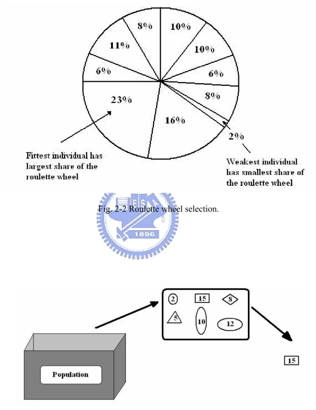
Selection operator is a process of deciding which chromosomes in the current population will pass their solution information to the next generation. For a genetic algorithms optimization process, the selection operator selects not only the currently best chromosomes but also some other chromosomes to avoid a local optimal solution. There are two popular selection strategies, roulette wheel selection and tournament selection [44].

The roulette wheel selection (Fig. 2-2) is the classical and simple selection scheme. As shown in Fig. 2-2, the roulette wheel selection selected chromosomes based on their probability. The probability was estimated as

∑

= = 1 i selection Fi Fj P (1-2)

where Fi is the fitness value of ith _{individual. For the roulette wheel selection, individuals}

with high fitness value will be selected more often than less fitness individuals, but it does not guarantee that the fittest member goes through to the next generation.

For tournament selection (Fig. 2-3), a subpopulation of N individuals is chosen randomly from the current population. Then the highest fitness of individual in the subpopulation wins the tournament and becomes the selected individual. The tournament size (N) can be changed to adjust the selection pressure. If the tournament size is larger, weak individuals have a smaller chance to be selected. The benefits of the tournament selection are (1) efficient to

code and (2) easy to adjust the selection pressure.

Moreover, a so called “elitism” process was commonly adopted to select the better individuals to pass to the next generation. The elitism process allows the better information to pass to next generation to get better solutions over times. It is essential, mainly for small population size.

2.1.4 Crossover

Crossover is a principal genetic operator for a genetic algorithm optimization procedure. The selection operator selects several individuals to be the parents and the crossover operator accepts a pair of parents’ solutions to generate two new individuals for the next generation population (Fig. 2-4). Many variations of crossover have been developed and the simplest one is one point crossover. As shown in Fig. 2-4(a), a cutting point was randomly selected in the parents’ chromosomes and the portion of the chromosomes of parents following the cutting point was changed to form two children. The cutting point can be one or more than one point (Fig. 2-4(b)). The selection of cutting point number is always depended on the optimization problem and population size.

2.1.5 Mutation

Mutation operator is analogous to biological mutation to avoid the loss of some important genes and increase the variation of the individuals. The individuals of new population were generated either directly copied or produced by crossover. In order to ensure that the individuals are not all exactly the same, a mutation operator is adopted to add new information into individuals occasionally. As shown in Fig. 2-5, one gene was selected randomly and flipped (0 becomes 1, 1 become 0).

A very small mutation rate may lead to a premature convergence of the genetic algorithm in a local optimum. A mutation rate that is too high may lead to loss of good solutions. In order to avoid the premature or the loss of good solutions, a fluctuated mutation rate was developed. A very small mutation rate was set in the beginning of optimization procedure to avoid the loss of good information and the mutation rate was increased when the candidate solution was convergenced to an optimal solution to avoid the premature.

2.2 Micro-genetic algorithm

The standard genetic algorithm is successfully applied to many different applications [21,22]. However, one major drawback is that the iterative global searching of the algorithm is time consuming. It will be deteriorating when additional iterations are needed in the smoothing procedure. There are many approaches to tackle this problem. For the genetic algorithm practice, reduction of the population size is an effective way. For conventional GA, the general choice of population size can range from 100 to 1000. This imposes a considerable loading on the computational time. To trade-off, the micro-genetic algorithm [17,20] is particularly adopted to accelerate the convergence of the conventional GA. The MGA is similar to the GA that proceeds with binary coded population and employs the selection and crossover operations to evolve population for generations, but with smaller population size than conventional GA. It had been reported that MGA reaches near optimal regions much earlier than the standard GA does [17]. Fig. 2-6 showed the flowchart of the micro-genetic algorithm.

The micro-genetic algorithm is a small population genetic algorithm. MGA uses a micro-population of five individuals [17]. It is well known that the GA works poorly with small population size due to insufficient information processing, which results in premature convergence to local optimal solutions. For the MGA, the best individual is passed to the new generation to ensure that the good individual is held, and it requires multiple convergences. The best individual of the old is remained and the others are randomly generated after each convergence. This operation is used to add new information and avoid premature convergence, and the mutation rate is set to zero.

Define coding and chromosome representation Population initialization Selection Crossover Mutation Converged? Optimal solution Probability calculation Evaluate fitness Evaluate fitness No Yes

Fig. 2-2 Roulette wheel selection.

(a)

(b)

Fig. 2-4 Crossover: (a) one point crossover and (b) two point crossover.

Define coding and chromosome representation Population initialization Selection Crossover Evaluate fitness Converged? Optimal solution Evaluate probability Evaluate fitness No Yes Create new population Evaluate fitness & probability State 1 State 2

Chapter 3 Surface function reconstruction

In order to generate a proper surface mesh and ensure the geometrical accuracy of the analytical model, the surface function is necessary during the surface mesh smoothing procedures. In some previous articles, the mesh smoothing procedures were applied to reposition the internal nodes on the plane (or tangent plane) of the primary elements, which is

C0-continuous [14,45]. It is based on an assumption that the primary surface elements were

well matched to the original surface. However, in this study, since the given data points may be chosen irregularly, the primary surface elements, which were triangulated directly from the

given data points, may not match the original surface well. Therefore, in this study, a C1

continuous surface function reconstruction algorithm was adopted to ensure the geometrical accuracy during the nodes repositioning.

There are many surface function reconstruction methods developed [23,46–51]. For a

finite element analytical model, a C1-continuous surface function is necessary for sufficient

numerical accuracy. Here, a C1 triangular patch interpolation method developed by Goodman

and Said [23] was adopted to reconstruct the surface function. It is a simpler and efficient method for the surface function reconstruction. In this method, surface function is reconstructed by local cubic Bezier triangular patches. The gradients of vertices are necessary for this surface function reconstruction procedure. We adopted a local derivative estimation method, which is also developed by Goodman et al. [52], to calculate the gradients of vertices.

3.1 Gradient estimation

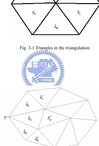
The gradients of surface nodes are calculated by the following approach: is a vertex

of a triangle and , are the triangles around (Fig. 3-1). We denote as the

gradient of the plane of . The gradient

V i t i=1,...k V g_i i t D_v of the node V is

∑

∑

= = = k i i k i i i v g D 1 1 λ λ (3-1)

where λ_i is the inverse of the area of the triangle . In (3-1) the node is assumed to be

in the interior of the domain. If the node is on the boundary of a domain, such as that in

Fig. 3-2, the gradient of the node is given by

i

t V

V

v

(

)

_∑

∑

= = ⎭⎬ ⎫ ⎩ ⎨ ⎧ ′ + ′ − ′ + = k i i i i i i i i i k i i v g g D 1 1 1 1 1 2 _λ λ λ λ λ λ λ (3-2)

which λ_i′ is the inverse of the area of the triangle t′, and _i t′ is the triangle which shares the _i

common edge of triangle t_i opposite to .

The value of can be estimated as the following: Let , be the

vertices of a triangle. Then the triangle can be written as V i g (xj,yj,zj) j=1,2,3 0 = + + +β γ δ αx y z (3-3)

where α, β and γ are the components of the normal vector of the triangle

) )( ( ) )( (y₂ −y₁ z₃ −z₂ − z₂ −z₁ y₃ −y₂ = α ) )( ( ) )( (z₂ −z₁ x₃ −x₂ − x₂ −x₁ z₃ −z₂ = β (3-4) ) )( ( ) )( (x₂ −x₁ y₃ −y₂ − y₂−y₁ x₃−x₂ = γ Then the gradient can be calculated as

⎟⎟ ⎠ ⎞ ⎜⎜ ⎝ ⎛_{− −} = ⎟⎟ ⎠ ⎞ ⎜⎜ ⎝ ⎛ ∂ ∂ ∂ ∂ = γ β γ α , , y z x z g_i (3-5)

3.2 Interpolation method

Consider a triangle with vertices , , in barycentric coordinates , ,

such that any point on the triangle can be expressed as

T V1 V2 V3 u v w 3 2 1 vV wV uV V = + + , u+v+w=1 (3-6)

We denote by the side opposite the vertex , from to (see Fig. 3-3). A cubic

Bezier triangular patch is then defined as

i

0 , 3 , 0 3 2 , 0 , 1 2 0 , 2 , 1 2 1 , 0 , 2 2 0 , 1 , 2 2 0 , 0 , 3 3 _{3 3 3 3} ) , , (u v w u b u vb u wb uv b uw b v b P = + + + + + 3 _{0,0,3 1,1,1} (3-7) 2 , 1 , 0 2 1 , 2 , 0 2 _{3 6} 3v wb + vw b +w b + uvwb +

where b_i,_j,_k are the triangular Bezier control points of P. The derivative of P with respect to the direction z=(z₁,z₂,z₃)= z₁V₁+z₂V₂ +z₃V₃, 0z₁ +z₂ +z₃ = is given by

3 2 1 z w P z v P z u P z P ∂ ∂ + ∂ ∂ + ∂ ∂ = ∂ ∂ (3-8)

We assume that function values are given and its first partial derivatives can be

calculated from Section 3.2.1. Then the derivative along the side can be calculated by

) (V_i F i e y F y y x F x x e F F _{i i i i} i ei _∂ ∂ − + ∂ ∂ − = ∂ ∂ = ( _{−1 +1}) ( _{−1 +1}) (3-9)

From the equation given above, we can determine the coordinates of all the control points

except . For example, following Equation (3-9) the three control points at vertex

can be decided as follows

k j i b, , b1,1,1 1 V ) ( 1 0 , 0 , 3 F V b = 3 ) ( ) ( ₁ 1 0 , 1 , 2 3 V F V F b = + e (3-10) 3 ) ( ) ( 1 1 1 , 0 , 2 2 V F V F b _{= −} e

Similarly we can obtain another six control points.

Let n_i be the inward normal direction to the edge e_i (see Fig. 3-3). Then

) , 1 , 1 ( _{1 1} 1 h h n = − − ) 1 , 1 , ( _{2 2 1} 2 = −h h − n (3-11) ) 1 , , 1 ( _{3 3} 3 h h n = − −

where 2 1 i i i i e e e h = − − ⋅ _{, i=1,2,3 (3-12)}

Hence, by using Equations (3-7) and (3-11) we can define the normal derivative on e_i as

2 0 , 3 , 0 1 , 2 , 0 1 0 , 3 , 0 0 , 2 , 1 1 )) ( ( 3b b h b b v n P − − − = ∂ ∂ +6(b1 b_0,2,1 h₁(b_0,1,2 b_0,2,1))vw (3-13) 1 , 1 , 1 − − − +3 2 2 , 1 , 0 3 , 0 , 0 1 2 , 1 , 0 2 , 0 , 1 ( )) (b −b −h b −b w

From (3-13), the linear normal derivative on e_i is

)) ( ( )) ( ( 2 1 _{0,2,1 1 0,1,2 0,2,1 1,2,0 0,3,0 1 0,2,1 0,3,0} 1 , 1 , 1 b h b b b b h b b b − − − = − − − +(1−h1)(2b0,2,1−b0,3,0 −b0,1,2)) (3-14) Then ) 2 ( ( 2 1 3 , 0 , 0 1 , 2 , 0 2 , 1 , 0 1 2 , 0 , 1 0 , 2 , 1 1 1 , 1 , 1 b b h b b b b = + + − − +(1−h1)(2b0,2,1−b0,3,0 −b0,1,2)) (3-15)

Similarly we can obtain 2 and . Finally, the interpolation function can be defined as

1 , 1 , 1 b 3 1 , 1 , 1 b 2 , 0 , 1 2 0 , 2 , 1 2 1 , 0 , 2 2 0 , 1 , 2 2 0 , 0 , 3 3 _{3 3 3 3} ) , , (u v w u b u vb u wb uv b uw b P = + + + + 3 , 0 , 0 3 2 , 1 , 0 2 1 , 2 , 0 2 0 , 3 , 0 3_{b 3v wb 3vw b w b} v + + + + (3-16) 2 2 2 2 2 2 3 1 , 1 , 1 2 2 2 1 , 1 , 1 2 2 1 1 , 1 , 1 2 2 6 v u u w w v b v u b u w b w v uvw + + + + +

3.3 Geometrical accuracy comparison

The comparison of geometrical accuracy for the original C0-continuous and our

enhanced C1-continuous surface can be shown as follows: thirty-six points and triangulation

in Whelan [46] were chosen (Fig. 3-4) and two test functions (Fig. 3-5) were employed: = ) , ( 1 x y F 0.75exp(₋((9_x−2)2 ₊(9_y−2)2)/4) ₊0.75exp(₋(9_x+1)2 /49₋(9_y+1)/10 ₊0.5exp(₋((9_x−7)2 ₊(9_y−3)2)/4) ₋0.2exp(₋(9_x−4)2₋(9_y−7)2) ) ) 1 3 ( 6 6 /( )) 4 . 5 cos( 25 . 1 ( ) , ( 2 2 x y = + y + x− F

The interpolated values of the test functions at a 25×25 uniform mesh points in a unit square

were computed and the maximum and mean errors. The computed surface errors were shown in Fig. 3-6 and Fig. 3-7 for test function 1 and test function 2 respectively. The surface errors,

shown in Table 3-1, indicate that the C1-continus surface is more accuracy than the

C0-continuous surface both on maximum and mean surface errors. Therefore, surface mesh

smoothing based on the reconstructed C1 surfaces is beneficial to enhance the geometrical

Fig. 3-1 Triangles in the triangulation.

Fig. 3-3 Notation of a triangle.

(a)

(b)

(a)

(b)

(a)

(b)

Table 3-1 Surface errors of the test functions for C0 and C1 surface reconstruction.

C0 surface C1 surface

Test function

Max. error Mean error Max. error Mean error

) , ( 1 x y F 0.215184 0.027594 0.120067 0.022945 ) , ( 2 x y F 0.059769 0.008789 0.035420 0.005101

Chapter 4. Surface mesh smoothing

4.1 Mesh generation

4.1.1 Triangular mesh generation

In general, finite element surface mesh is generated based on prescribed patch interpolation by adopting the Delaunay Triangulation [5] or Advancing Front Methods [6]. However, the generation of surface mesh based on unorganized points set is necessary in some science and engineering fields, where geometrical data is often measured or generated at isolated and unorganized positions, such as mentioned earlier of the biomedical research. In this application, the given data is just the points set and the surface function is yet to be defined. Therefore, the surface mesh can not be generated based on its surface function directly. For this application, a common way to reconstruct the surface model is to triangulate the given points [7-10]. The triangulation procedure aims at generating a primary triangular surface mesh as well as creating background triangular patches for the use in surface function reconstruction procedure. Furthermore, since the distribution of the given points may be irregular over the surface of the model, the primary triangular meshes always contain some ill-posed triangles. Therefore, some mesh cleanup operations [53] were introduced to improve the topological connectivity of the triangular meshes, and then MGA approach was applied to enhance the mesh quality further.

4.1.2 Quadrilateral mesh generation

Once the primary triangular surface mesh was created, the quadrilateral surface mesh can be generated based on the triangular one. The conversion scheme [4,45,54-56] was employed to serve this purpose. It is a common and convenient way to generate an unstructured quadrilateral mesh. The quadrilateral mesh was created by a careful process to merge two adjoining triangles to form a quadrilateral element. However, the conversion scheme usually introduces plenty of ill-posed quadrilaterals. To improve the mesh quality, a two-stage procedure is required. First, mesh structure modification (topological improvement) operations [57,58], such as edge swapping, node elimination and edge dividing, were employed to refine the mesh connectivity. Then the mesh quality was further enhanced by

applying the MGA approach.

4.1.3 Mesh structure modification operations

For the finite element mesh generation, the ideal numbers of elements connected to a node are six and four for triangular and quadrilateral mesh respectively. Generally, the bad nodes, which were connected with more than or less than the ideal number of elements, were treated before mesh smoothing procedure. In this section, we presented three basic mesh structure modification operations to tackle these bad nodes.

1. Edge swapping

This operator swaps an edge adjacent to two elements. It is used to adjust the number of surrounding elements of the connected nodes. As shown in Fig. 4-1(a), the number of

elements connected to node a (Na) and node b (Nb) are seven, which are more than the ideal

number of triangular elements. Therefore, the interior edge was swapped to improve this mesh

structure. In Fig. 4-1(b), Nb and Ne are five, which are more than the ideal number of

quadrilateral elements, and the interior edge (edge be ) was swapped (edge cf ) to modify

this mesh structure. 2. Node eliminating

This operator eliminates nodes whose number of surrounding elements is less than the

ideal number. As shown in Fig. 4-2(a), Nd is three and it is an improper node. For this

situation, the node d is eliminated to exclude the improper node. Figure 4-2(b) shows the improper node g with three surrounding quadrilateral elements and the mesh structure will be improved by eliminated the improper node g.

3. Edge dividing

This operator divides edge by inserting a new node on the center of a long edge. In Fig. 4-3(a), the edge bd is longer than others. Then a node f was inserted to the center of edge bd and the nearby edges were rearranged to improve the triangular mesh quality locally. Similarly, the longest edge be in Fig. 4-3(b) was divided by inserting a new node g on the

center and the elements connected to it were rearranged too.

There are many mesh structure modification operations presented in the previous articles [53,57,58]. These operations were based on the three basic operations, edge swapping, node elimination and edge dividing. Please refer to [53], [57] and [58] for the details of the mesh structure modification operations.

4.2 Micro-genetic algorithm surface mesh smoothing

In this thesis, the given surface mesh was triangular mesh and/or converted the triangular mesh into quadrilateral mesh. The surface mesh was first refined by the mesh structure modification operators [53,57,58], and then the MGA mesh smoothing procedures were applied to enhance the surface mesh quality further. The procedures of our surface mesh smoothing and the MGA adopted in our scheme were summarized as follows:

Step 1) Input data: Input the data of primary mesh, which includes surface function, node positions and element connectivity. If the surface function is not given, the gradients of nodes will estimated by the gradients estimation procedures [52].

Step 2) MGA mesh smoothing begins:

Step 3) Search the optimal solutions within each adjacent element by using Step 4 to Step 7 and then choose the best one to be the new position of the node.

Step 4) Initial population: The MGA requires multiple convergences. According to the reference [17], a population size of five is chosen in each convergence. The best individual of the previous generation will be held. The others are generated randomly.

Step 5) Decode the strings and calculate their node positions based on the reconstructed surface function (Section 3.2). Calculate their fitness values and then carry the best string to the next generation.

Step 6) Select four strings (contains the best string) for reproduction by employing the roulette wheel strategy [21]. Generate four individuals by employing the crossover operator with probability of one [17].

Step 7) Check the convergence criterion. If it is not convergence, go to step 5 or else go to step 3 or step 4.

Step 9) Check the convergence of the whole mesh smoothing procedures. If it is not convergence, go to step 2 or else end off the smoothing procedures.

4.2.1 Design parameters

In the MGA mesh smoothing procedures, the design parameters were chosen to represent the nodes position. In order to avoid degenerate elements, the search space was restricted within a triangular area for each adjacent element in both triangular and quadrilateral mesh smoothing. To represent a node lay on a triangle, we choose two parameters and , which relate to the barycentric coordinates as the following: Consider a triangle

1

r r₂

T (Fig. 4-4)

with vertices , and in barycentric coordinates , and , such that any point

on the triangle can be expressed as

1 V V₂ V₃ u v w 3 2 1 vV wV uV V = + + , u+v+w=1 (3-17) Now, with 0< <1, r_i i=1,2, the barycentric coordinates can be given as

2 2 1 2 1(1 r ) (1 r)(1 r ) 1 r r u= − + − − = − ) 1 ( ₁ 2 r r v= − (3-18) 2 1r r w=

Substituting (3-18) into (3-17), we get

3 2 1 2 1 2 1 2) (1 ) 1 ( r V r r V rrV V = − + − + (3-19)

As shown in Fig. 4-4, the vertices , and are collinear when =1. To avoid

that, we let 0< <0.5. After the position of point V is obtained, the exact position is calculated by mapping it to the original surface based on its corresponding triangular patch and the local reconstructed surface function (Section 3.2).

1

V V₂ V₃ r₂

2

r

In this study, the fitness function is a criterion to judge the mesh quality and defined with the mesh quality measurement index. For the triangular mesh quality measurement, the common used quality index is

2 2 2 _{|| || || ||} || || || || 3 2 AC BC AB AC AB + + × = α (3-20)

where A, B, are the vertices of a triangle. According to this mesh quality measurement,

the fitness function for the triangular mesh smoothing is defined as

C t F

∑

= = n i i t F 1 α (3-21)

where is the number of adjacent triangular elements. n

For the quadrilateral mesh quality measurement, Knupp [59] presented an algebraic mesh quality metrics from the Jacobian matrix. The definition of quadrilateral shape quality metric is as follows: for a plane quadrilateral element, let the coordinates of the four nodes be (x_k,y_k), =0,1,2,3. The Jacobian matrices, k A_k, one at each node of the quadrilateral:

⎟⎟ ⎠ ⎞ ⎜⎜ ⎝ ⎛ − − − − = + + + + k k k k k k k k k _{y y y y} x x x x A 3 1 3 1 (3-22)

where the indices k+1 and k+3 are taken modulo four, for example, if =1 then k k+3

becomes 0. Four metric tensors are obtained by the combinations T _k. Let , ,

kA

A λkij i j =1,2, be

the th component of the th metric tensor. Geometrically, at the th node, is the

square of the length of the side connecting nodes and

ij k k k

11

λ

k k+1, is the square of the

length of the side connecting nodes and

k

22

λ

k k+3. Let θ_k be the angle between the two

sides joined at the th node, the quadrilateral shape quality metric can be expressed as k

∑

= + = ₃ 0 2_{)/( sin )} 1 ( 8 k rk rk θk β (3-23)

where r = λ₂₂/λ₁₁ is the length ratio of kth _{node. This concept can be extended to}

measure quadrilateral surface mesh quality directly. Then the fitness function for the quadrilateral mesh smoothing Fq is defined as

∑

= = n i i q F 1 β (3-24)

where is the number of adjacent quadrilateral elements. n

4.3 Surface mesh smoothing results

The proposed approach is tested in several unorganized point datasets. A simple geometry of saddle shape with prescribed surface function is used to validate the procedure and to compare the performance of our MGA approach and the conjugate gradient method (Table 4-1). It is then applied to complicated geometries, such as wing-fuselage, which is often used in preliminary aircraft design, and biological dataset of shapes of a foot and a rat, which are constructed from contours by a three dimensional laser scanning and from a sequence of segmented bio-images respectively. The geometrical reconstruction of bio-images is a crucial pre-processing for physical modeling in biology and biomechanics. So, the applications are used to demonstrate not only the effectiveness but also the practical use of our approach. In order to show the capability of our MGA mesh smoothing approach, all of the smoothed results are obtained by smoothing the primary meshes directly without any additional mesh treatment. The mesh quality is measured according to the Section 4.2 that the

triangular mesh quality index is α and the quadrilateral mesh quality index is β. The results

are summarized in Table 4-2 and 4-3 for triangular and quadrilateral surface meshes respectively. Significant enhancement is found by our approach. Furthermore, in the Table 3-4, the worst quadrilateral mesh quality is set as 0.0001, which represents that one of theinterior

angle is greater than 1790 and the codes are run in Linux PC with a dual core AMD 2 GHz

CPU and 3 GHz RAM.

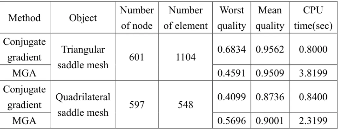
The first example is a basic mathematical function of saddle shape (Fig. 4-5), which allows us to scrutinize the performance of the approach. The surface function is denoted as the following:

4

10 2

2 _y

x

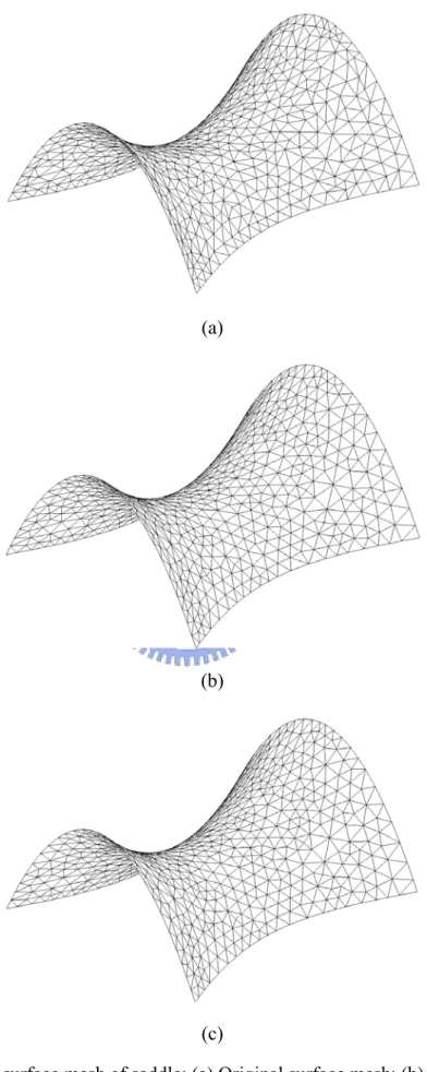
z = − (3-25) The saddle shape surface, unlike the usual well-behaved elliptic shape, has negative curvature, which is appealing to be used as a test case for the surface smoothing [60]. The triangular surface mesh is generated based on Delaunay triangulation and the quadrilateral surface mesh converted from the triangular mesh (Section 4.1). The performance of MGA can be observed by comparing with that of the conjugate gradient method in the saddle shape. The Table 4-2 shows that the improvement of the mean quality of triangular mesh reaches to 0.9562 and 0.9509 by both approaches, but the CPU time of our MGA approach is approximate five times of the conjugate gradient method. This is one drawback of GA, but can be easily tackled by parallelism and there are several parallel GA [24] developed with great success. The approach is similarly employed to the quadrilateral mesh. Our quadrilateral meshes are generated using a popular conversion scheme or fission scheme [4,45,54-56]. The conversion scheme essentially merges two neighboring triangles to form a new quadrilateral. This method may introduce ill-posed quadrilaterals, and needs further treatments [57,58] for practical use. The Table 4-3 shows that the improvement of mean quality of quadrilateral mesh reaches to 0.8736 and 0.9001 by employing the conjugate gradient method and our MGA approach respectively. It is clear that our performance as a global method achievement for mesh quality improvement is better than the conjugate gradient method. The enhancements of the mesh quality can be also visually observed from Fig. 4-5 and Fig. 4-6 for triangular and quadrilateral surface mesh respectively.

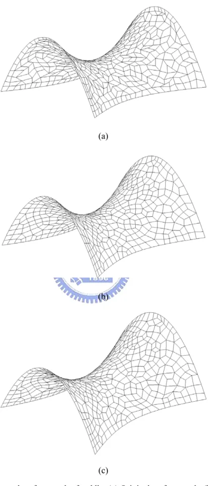
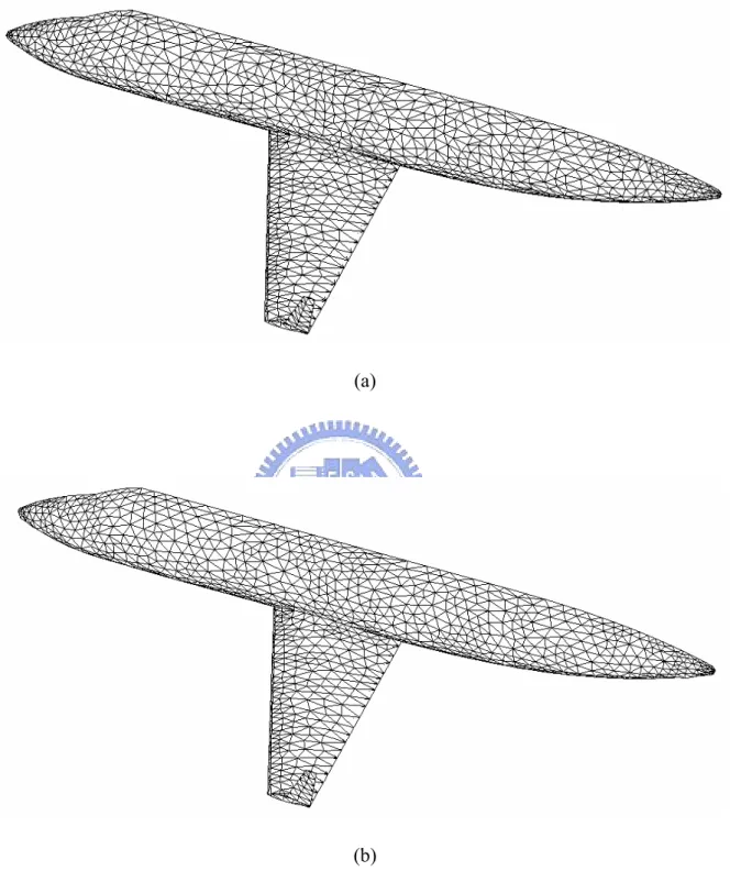
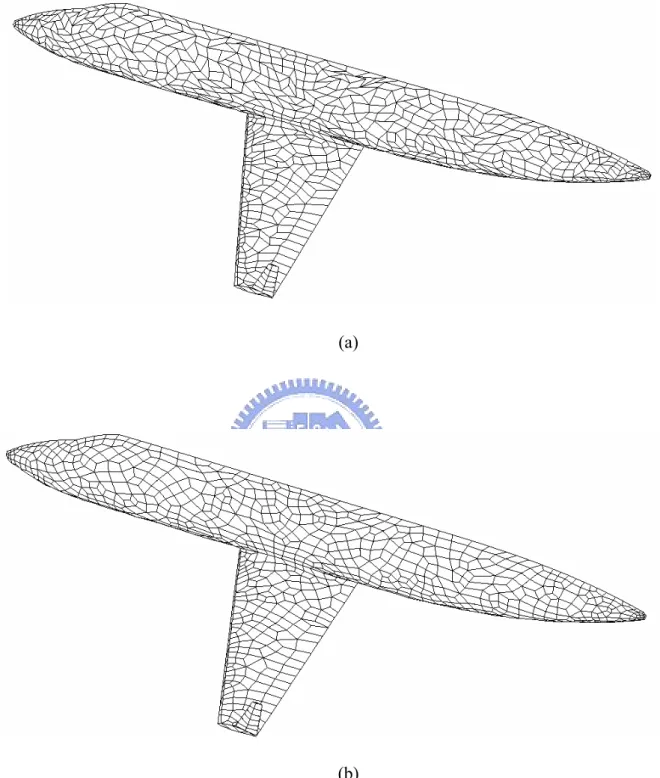
The following example is a complicated geometry of wing-fuselage configuration of NCKU-ILD-101 [61]. Such kind of geometrical model is often used in CFD simulation for aircraft preliminary design. The usual practice for generating a surface mesh for such a geometrical model is based on a pre-defined patch interpolation. The current data is prepared from a point datasets that is well generated by usual mesh generation methods of Delaunay triangulation. The point datasets are deliberately reduced from 9,962 points to 1,314 points, but the feature of the geometry is carefully preserved by using AMIRA [62]. The reduction makes mesh so coarse that it is difficult to maintain quality for simulation. However, it is well suited to test the performance of the current MGA procedure. The points at the edges and joints have to be marked and fixed to avoid singularity during the smoothing. The results are shown in Fig. 4-7 and Fig. 4-8 for triangular and quadrilateral meshes respectively. The improvement is significant, which can be seen from the quality indices measured in Table 4-2 and 4-3. The mean quality index of triangular mesh is enhanced from 0.8483 to 0.9046. It is

well known that quadrilateral mesh is less stiff than triangular mesh and allows more degrees of freedom to move the mesh to change the shape of elements. As a result, it needs more smoothing treatments after generating the surface mesh. Our results show significant improvement in terms of worst and average property measured within elements. The mean and worst qualities are enhanced from 0.6982 to 0.8580 and 0.0001 to 0.4215 respectively.

Due to the advance of image processing, geometry reconstruction and mesh generation, nowadays larger and more complicated geometry models can be reconstructed from a sequence of bio-medical images data set. The need for such reconstruction is immense and it has become a common practice for bio-medical and bioengineering study. By scrutinizing the reconstruction procedure for such geometry models, it can be found that the surface geometry is usually defined by a set of unorganized points, or at least by a sequence of un-associated contours, that is identified by pattern recognition methods on each image of interest. The surface triangulation is not straightforward. It is even more challenging for surface mesh quality enhancement in that the re-arrangement of the point distribution needs higher order interpolation methods for accuracy. Two test cases are given to demonstrate the capability of the proposed methods for tackling these challenging issues.

The first example is the foot shape model of Polhemus [63]. The original model was created by using FastSCAN with the FastRBF Extensions. The surface data points are measured by the laser scanner FastSCAN, and then the data points are reconstructed to form the geometrical model by the software FastRBF Extensions. It is a very convenient and efficient way to reconstruct a geometrical model, especially when the surface function is not pre-defined, by using a laser scanner system. In this study, the original foot model contains 25,845 nodes. Similarly the original data points are reduced to 4,039 and it contains 8,000 triangles on the surface. Our MGA approach constructs a high order interpolation and iteratively optimizes the point distribution in terms of local evolution. The triangular mesh quality was enhanced as expected from0.8275 to 0.9192 (Fig. 4-9). The original surface mesh obtained is actually well defined. However, the current approach can still give further enhancement of the mesh quality. For systematical comparison, the quadrilateral mesh is generated and smoothed in a similar fashion. The results of obvious improvement are as expected that the surface quadrilaterals are more regular after the MGA approach (Fig. 4-10). This also can be readily observed from the mean quality, which is improved from 0.7049 to 0.8632 (Table 4-3).

The last case is a rat shape that is reconstructed from a sequence of image slices of histological sections from Ryutaro Himeno of RIKEN [64]. The original reconstructed model

contains skin, bone, organs and so on, and it can help people to observe the whole model of rat virtually without dissect a real rat. This approach can be used to reconstruct more models of biology. In this study, we extract the skin model and reduce it by using AMIRA. As shown in Fig. 4-11, this model contains 25,670 nodes and 51,354 elements. The reconstructed shape is rough and irregular and the primary surface mesh contains many poor triangles elements. Some of the nodes connect to 3 elements and others connect to more than 9 elements. The poor connectivity is treated first by the mesh structure modification operators [53,57,58]. To avoid interpolation error, the singular points, which locate at the boundary or contain large curvature variation, need be identified and fixed before the surface mesh smoothing. The MGA procedure is then used to re-construct surface interpolation function and to smooth the mesh by optimizing the point distribution. The result is shown in Fig. 4-11(b) and the mean mesh quality improved from 0.8963 to 0.9453. The similar improvement for quadrilateral mesh can be found in Fig. 4-12 and Table 4-3.

(a) (b)

Fig. 4-1 Edge swapping: (a) triangular elements and (b) quadrilateral elements.

(a) (b)

(a) (b)

Fig. 4-3 Edge dividing: (a) triangular elements and (b) quadrilateral elements.

Table 4-1. The comparison between conjugate gradient method and MGA method using the saddle geometry.

Method Object Number

of node Number of element Worst quality Mean quality CPU time(sec) Conjugate gradient 0.6834 0.9562 0.8000 MGA Triangular saddle mesh 601 1104 0.4591 0.9509 3.8199 Conjugate gradient 0.4099 0.8736 0.8400 MGA Quadrilateral saddle mesh 597 548 0.5696 0.9001 2.3199

Table 4-2. Mesh quality improvement for the triangular surface meshes.

Object Number of node Number of element Worst quality Mean quality CPU time(sec) original 0.2535 0.8483 smoothed Wing- fuselage 1419 2432 0.2535 0.9046 3.0500 original 0.3803 0.8275 smoothed Foot 4039 8000 0.3469 0.9192 23.8200 original 0.2225 0.8963 smoothed Rat 25670 51354 0.2460 0.9453 150.0509

Table 4-3. Mesh quality improvement for the quadrilateral surface meshes.

Object Number of node Number of element Worst quality Mean quality CPU time(sec) original 0.0001 0.6982 smoothed Wing- fuselage 1405 1200 0.4215 0.8580 4.1000 original 0.0001 0.7049 smoothed Foot 4010 3971 0.4111 0.8632 19.6400 original 0.0001 0.7568 smoothed Rat 25374 25383 0.2553 0.8899 88.8099

(a)

(b)

(c)

Fig. 4-5 Triangular surface mesh of saddle: (a) Original surface mesh; (b) Surface mesh after MGA smoothing; and (c) Surface mesh after conjugate gradient smoothing.

(a)

(b)

(c)

Fig. 4-6 Quadrilateral surface mesh of saddle: (a) Original surface mesh; (b) Surface mesh after MGA smoothing; and (c) Surface mesh after conjugate gradient smoothing.

(a)

(b)

Fig. 4-7 Triangular surface mesh of wing-fuselage: (a) Original surface mesh and (b) Surface mesh after smoothing.

(a)

(b)

Fig. 4-8 Quadrilateral surface mesh of wing-fuselage: (a) Original surface mesh and (b) Surface mesh after smoothing.

(a) (b)

Fig. 4-9 Triangular surface mesh of foot: (a) Original surface mesh and (b) Surface mesh after smoothing.

(a) (b)

Fig. 4-10 Quadrilateral surface mesh of foot: (a) Original surface mesh and (b) Surface mesh after smoothing.

(a)

(c) (d)

Fig. 4-11 Triangular surface mesh of rat: (a) Original surface mesh; (b) Surface mesh after smoothing; (c) Original surface mesh (enlarged); and (d) Surface mesh after

(a)

(c) (d)

Fig. 4-12 Quadrilateral surface mesh of rat (a) Original surface mesh (b) Surface mesh after smoothing (c) Original surface mesh (enlarged) (d) Surface mesh after