減少IMS現狀資訊訊息流量之弱一致性方法

國

立

交

通

大

學

網路工程研究所

碩

士

論

文

減少 IMS 現狀資訊訊息流量之弱一致性方法

A Weakly Consistent Scheme for IMS Presence Service

研 究 生：劉仁煌

指導教授：林一平 教授

陳懷恩 教授

減少 IMS 現狀資訊訊息流量之弱一致性方法

A Weakly Consistent Scheme for IMS Presence Service

研 究 生：劉仁煌 Student：Ren-Huang Liou

指導教授：林一平博士 Advisor：Dr. Yi-Bing Lin

指導教授：

陳懷恩博士

Advisor：

Dr. Whai-En Chen

國 立 交 通 大 學

網 路 工 程 研 究 所

碩 士 論 文

A Thesis

Submitted to Institute of Network Engineering College of Computer Science

National Chiao Tung University in partial Fulfillment of the Requirements

for the Degree of Master

in

Computer Science

June 2009

Hsinchu, Taiwan, Republic of China

減少IMS現狀資訊訊息流量之弱一致性方法

學生：劉仁煌

指導教授： 林一平博士

陳懷恩博士

國立交通大學網路工程研究所碩士班

摘

要

在 第 三 代 行 動 通 訊 系 統 UMTS (Universal Mobile Telecommunications System)中， 現 狀 資訊服務(Presence Service)是由 IP多媒體子系統(IP Multimedia Core Network Subsys-tem; IMS)負 責 提 供。 在 IMS中， 現 狀 資 訊 伺 服 器 (Presence Server)負 責 將 更 新 後 的 現 狀 資 訊 (Presence Information) 通 知 給 已 授 權 的 觀 看 者 (Watcher)。 如 果 現 狀 資 訊 更 新 的頻率比觀看者瀏覽的頻率還要高，現狀資訊伺服器會產生許多不必要的通知訊息 (Notification)。本論文實作一完整即時訊息與現狀資訊服務系統。在此實作，本論文 使用一個弱一致性的方法，稱為延遲更新(Delayed Update)，來減少發送通知訊息造 成的流量。此方法使用一個計時器來控制傳送通知訊息的頻率。本論文針對延遲更新 進行效能分析。研究結果顯示，延遲更新可以有效減少發送通知訊息造成的流量，而 且不會嚴重降低觀看者看到錯誤資訊的機率。 關鍵字： 延遲更新, IP多媒體子系統, 現狀資訊服務

A Weakly Consistent Scheme for IMS Presence Service

Student: Ren-Huang Liou

Advisors: Prof. Yi-Bing Lin

Prof. Whai-En Chen

Institute of Network Engineering

National Chiao Tung University

ABSTRACT

IP Multimedia Core Network Subsystem (IMS) provides presence service for Universal Mobile Telecommunications System (UMTS). In IMS, the presence server is responsible for notify-ing an authorized watcher of the updated presence information. If the updates occur more frequently than the accesses of the watcher, the presence server will generate many unneces-sary notifications. In this thesis, we implemented an instant messaging and presence service system. In our implementation, we use a weakly consistent scheme (called delayed update) to reduce the notification traffic. In this scheme, a delayed timer is defined to control the notification rate. We propose an analytic model and simulation experiments to investigate the performance of delayed update. The study indicates that delayed update can effectively reduce the notification traffic without significantly degrading the valid access probability.

Keywords: Delayed Update, IP Multimedia Core Network Subsystem (IMS), Presence Service

誌

謝

Contents

1.1 Implementation of Instant Messaging and Presence Service System . . . 2

1.2 Organization . . . 3

2 Message Flows for IMS Presence Service 5 2.1 Subscription Procedure . . . 5

2.2 Publication Procedure . . . 6

2.3 Notification Procedure . . . 6

3 Input Parameters and Output Measures 9

4 Derivation for E[N ] and p 12

5 Simulation Validation 15 6 Numerical Examples 18 7 Conclusions 21 7.1 Contribution . . . 21 7.2 Future Work . . . 22 Bibliography 23

A An Alternative Derivation for p 25

A.1 Fixed Delayed Threshold . . . 26 A.2 Exponential Delayed Threshold . . . 26

B Simulation Model 28

List of Tables

5.1 Comparison of Analytic and Simulation Results under Different µ Values (λ = γ, Va = 1/µ2, and Vu = 1/λ2) . . . 16

5.2 Comparison of Analytic and Simulation Results under Different Vu Values

(λ = γ = µ and Va = 1/µ2) . . . 17

List of Figures

1.1 The UMTS Network Architecture for Presence Service . . . 2

1.2 Instant Messaging and Presence Service System . . . 3

1.3 The User Interface of Instant Messaging and Presence Service Client . . . 4

2.1 The Subscription Procedure . . . 6

2.2 The Publication Procedure . . . 7

2.3 The Notification Procedure . . . 7

3.1 Timing Diagram for Delayed Update . . . 10

6.1 Effects of γ/λ and Vu on p . . . . 19

6.2 Effects of γ/λ and Vu on E[N ] . . . . 20

Chapter 1

Introduction

Presence service allows an Internet user to access another user’s presence information includ-ing the user status, the activities (e.g., workinclud-ing, playinclud-ing, etc.), the email/phone addresses, and so on. This service is typically utilized together with the instant messaging applications such as Windows Live Messenger.

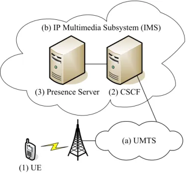
In Universal Mobile Telecommunication System (UMTS), presence service is provided through IP Multimedia Core Network Subsystem (IMS) [2, 8]. Figure 1.1 illustrates a simplified UMTS network architecture for presence service [1]. In this architecture, a user with a User Equip-ment (UE; Figure 1.1 (1)) accesses presence service in IMS (Figure 1.1 (b)) via the UMTS (Figure 1.1 (a)). The user plays the role as a presentity when he/she provides information to the presence server (Figure 1.1 (3)). On the other hand, the user is called a watcher if he/she accesses other users’ information from the presence server. In IMS, Call Session Control Function (CSCF; Figure 1.1 (2)) is responsible for carrying out the control signaling. As an IMS application server, the presence server stores the information of the presentities, and determines the authorized watchers who can access the presence information.

(a) UMTS (2) CSCF (3) Presence Server

(b) IP Multimedia Subsystem (IMS)

(1) UE

Figure 1.1: The UMTS Network Architecture for Presence Service

1.1

Implementation of Instant Messaging and Presence

Service System

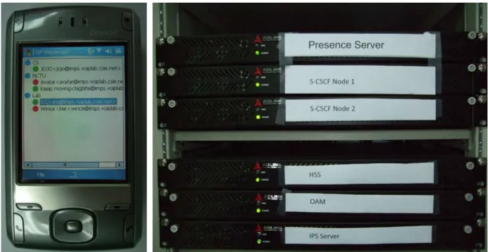
3rd Generation Partnership Project (3GPP) defines the presence service procedures for IMS. Based on 3GPP standards, we have implemented an instant messaging and presence service (IMPS) system including a presence server and an IMPS client (as illustrated in Figure 1.2). The presence server is implemented using the C language, which runs on the ADLINK In-dustrial Computer RK110SB-D3S2-852LV-3.0M4G with the Linux operating system. On the other hand, the IMPS client is written using the C++ language, which runs on the Dopod 838 with the Microsoft Windows Mobile platform.

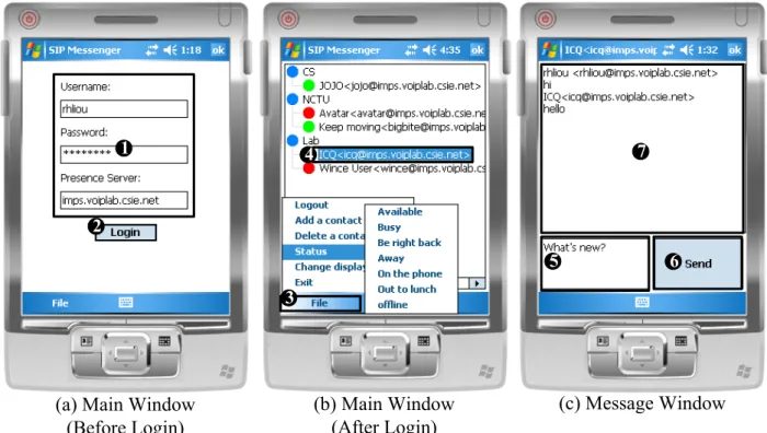
Figure 1.3 shows the user interface of the IMPS client, which consists of two windows. The Main window (Figure 1.3 (a)) is popped up after the IMPS client program is executed. It waits for the user to input the username, the password, and the address of the presence server (Figure 1.3 (1)). After the user clicks the Login buttom (Figure 1.3 (2)), the IMPS client ex-ecutes the presence service procedures to be described in Chapter 2. After the user logins the presence service, the Main window shows the user’s contact list (Figure 1.3 (b)). Each item in the contact list represents a user’s friend. The friend’s status is represented by a status icon

Figure 1.2: Instant Messaging and Presence Service System

(e.g., the green icon means that the status is available). The user can add/delete a contact through the File menu (Figure 1.3 (3)). The File menu also offers the following commands: logout the presence service, change status, change display name, and exit the program. When the user wants to contact his/her friend, the user clicks the corresponding item (Figure 1.3 (4)) in the contact list. Then, the Message window (Figure 1.3 (c)) is popped up. The user types a message in the Input Text area (Figure 1.3 (5)), and sends it by clicking the Send buttom (Figure 1.3 (6)). The Message Log area (Figure 1.3 (7)) displays the message history.

The above implementation won the 3rd place at Ministry of Education (MoE) Communi-cation Competition Contest 2006, and won the 2nd place at National Chiao Tung University (NCTU) Computer Science (CS) Senior Project Contest 2006.

1.2

Organization

The 3GPP presence service procedures may incur large traffic that significantly consumes the limited radio resources and UE power. To resolve this issue, many mechanisms have been proposed [9]. In this thesis, we consider a weakly consistent scheme called delayed update

(c) Message Window (a) Main Window

(Before Login) 1 2 5 6 7 4 (b) Main Window (After Login) 3

Figure 1.3: The User Interface of Instant Messaging and Presence Service Client exercised at the presence server to reduce the presence traffic between a watcher and the presence server. In this scheme, the UE needs not be modified.

This thesis addresses the issue of reducing the network traffic in the IMS presence service. This thesis is organized as follows. Chapter 2 describes the message flows for the 3GPP IMS presence service, and then introduces delayed update. Chapter 3 describes the input param-eters and output measures for modeling delayed update. Chapters 4-5 propose an analytic model to study the performance of delayed update. Chapter 6 investigates delayed update by numerical examples, and the conclusions are given in Chapter 7.

Chapter 2

Message Flows for IMS Presence

Service

This chapter describes the message flows for the 3GPP presence service procedures including the subscription, the publication, and the notification [1, 3]. These procedures are imple-mented by utilizing Session Initiation Protocol (SIP) [10, 11, 12, 16]. Then we introduce delayed update for reducing the notification traffic.

2.1

Subscription Procedure

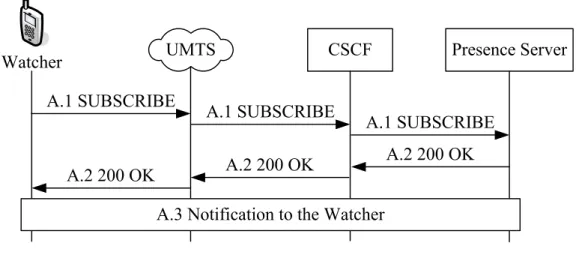
When a watcher attempts to access the presence information of other users (i.e., the pre-sentities), the subscription procedure is executed. In our implementation (see Section 1.1), the subscription procedure is triggered when the user logins the presence service. Figure 2.1 illustrates the subscription message flow between the watcher and the presence server. Detailed steps are described as follows:

Step A.1: The watcher (i.e., a UE) issues a SIP SUBSCRIBE message to the presence server

through the UMTS and the CSCF.

Step A.2: After verifying the identify of the watcher [4], the presence server sends a 200

OK message to the watcher. The message indicates that the watcher is authorized to subscribe to the presence information.

Presence Server CSCF

A.1 SUBSCRIBE A.2 200 OK

A.3 Notification to the Watcher UMTS A.1 SUBSCRIBE A.1 SUBSCRIBE A.2 200 OK A.2 200 OK Watcher

Figure 2.1: The Subscription Procedure

Step A.3: The presence server sends the presence information to the watcher through the

notification procedure to be described in Figure 2.3.

2.2

Publication Procedure

The publication procedure is executed when a presentity changes his/her presence informa-tion (e.g., the activity is changed from “playing” to “working”). Figure 2.2 illustrates the publication message flow with the following steps:

Step B.1: A SIP PUBLISH message is issued by the presentity to the presence server through

the UMTS and the CSCF. This message contains the updated presence information.

Step B.2: After the presence server received this SIP PUBLISH message, it stores the

pres-ence information in association with this presentity, and returns the 200 OK message. This message indicates that the publication is successful.

2.3

Notification Procedure

The presence server pushes the subscribed presence information to an authorized watcher through the notification procedure when the information is updated. Figure 2.3 illustrates

Presence Server CSCF B.1 PUBLISH B.2 200 OK UMTS B.2 200 OK B.1 PUBLISH B.1 PUBLISH B.2 200 OK Presentity

Figure 2.2: The Publication Procedure

C.1 NOTIFY CSCF C.2 200 OK UMTS C.1 NOTIFY C.1 NOTIFY C.2 200 OK C.2 200 OK Presence Server Watcher

Figure 2.3: The Notification Procedure the notification message flow with the following steps:

Step C.1: The presence server sends a SIP NOTIFY message to the watcher through the

CSCF and the UMTS. This message contains the modified presence information.

Step C.2: The watcher returns the 200 OK message to indicate that the presence

informa-tion is successfully received.

Note that the notification procedure is a “push” action. A watcher may access the presence information through “pull” action such as the poll-each-read mechanism. The details can be found in [7].

2.4

Delayed Update

The presence server immediately notifies a watcher of the presence information updates. If the updates occur more frequently than the accesses of the watcher, then the presence server will generate many notifications. A weakly consistent scheme called delayed update can be used to reduce the notification traffic between the presence server and the watcher (i.e., Steps C.1 and C.2 in Figure 2.3).

In delayed update, when the presence server receives the updated presence information (i.e., Step B.1 in Figure 2.2), the watcher is not notified of the updated information immediately. Instead, the presence server starts a delayed timer with a period T . This period is referred to as the delayed threshold. If the presence information is updated again within period T , the old information in the presence server is replaced by the new one. When the timer expires, the presence server notifies the watcher of the presence information (i.e., Step C.1 in Figure 2.3 is executed). Therefore, the notifications for the updates in T are saved. On the other hand, if an access occurs at any time in T , the watcher may access the obsolete information. RFC 3856 describes a mechanism similar to delayed update, where T = 5 seconds [13]. How-ever, this default delayed threshold value may not fit all user activities, and it is important to select an appropriate T value such that notification traffic is reduced while the watcher only occasionally accesses the obsolete presence information.

Chapter 3

Input Parameters and Output

Measures

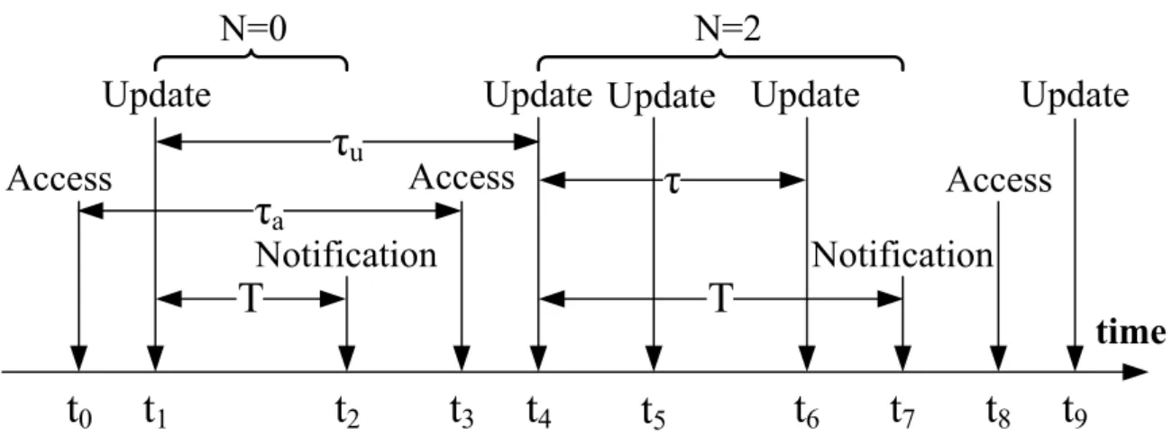
This chapter describes the input parameters and output measures for modeling delayed up-date. Figure 3.1 illustrates a timing diagram where the watcher accesses the presence infor-mation at t0, t3, and t8. The presence information is updated at t1, t4, t5, t6, and t9. At

t2 and t7, the presence server notifies the watcher of modified presence information. In this

figure, the delayed threshold T = t2 − t1 (also t7 − t4) is a random variable with the mean

1/γ. Let N be the number of update messages occurring during T . In this example, N = 0 in [t1, t2], and N = 2 in [t4, t7]. The inter-access interval τa = t3− t0 (also t8− t3) is a random

variable with the mean 1/µ and the variance Va. Let the inter-update interval τu = t4− t1

(also t5 − t4, t6 − t5, and t9− t6) be a random variable which has density function fu(τu),

the mean 1/λ, the variance Vu, and Laplace transform fu∗(s). Let τ = t6− t4 be the interval

between the first update message and the last update message occurring in T . We define an observation interval as a period between when the delayed threshold begins and when the first update message occurs after the end of the delayed threshold. In Figure 3.1, [t1, t4] and

[t4, t9] are the observation intervals.

Access

Access

Update

Update

Notification

T

Notification

time

Update

τ

N=0

Update

N=2

Update

t

t

t

t

t

t

t

t

t

t

τ

Access

τ

T

Figure 3.1: Timing Diagram for Delayed Update

• p: the probability that the watcher accesses the valid presence information. In Figure 3.1, an access is valid if it occurs in [t2, t4] and [t7, t9].

• E[N]: the expected number of update messages occurring in T .

It is clear that the update messages occurring in T are the saved notification messages. There-fore, the larger the p and the E[N ] values, the better the performance of delayed update.

The notation used in this thesis is summarized below. • T : the delayed threshold.

• p: the probability that the watcher accesses the valid presence information.

• N: the number of update messages occurring in T .

• τu: the inter-update interval of the presence information.

• τ: the interval between the first update message and the last update message occurring in T .

• τa: the inter-access interval of the watcher.

• 1/λ = E[τu]: mean inter-update interval.

• 1/µ = E[τa]: mean inter-access interval.

• Va: the variance for the τa distribution.

• Vu: the variance for the τu distribution.

• fu(·): density function for the τu distribution.

• f∗

Chapter 4

Derivation for E[N ] and p

This chapter describes an analytic model for deriving E[N ] and p. If the inter-update interval τu has the exponential distribution with the mean 1/λ, then due to the Poisson property of

the update arrivals, for a delayed threshold T with an arbitrary distribution with the mean 1/γ, the expected number E[N ] of update messages occurring in this period is

E[N ] = λE[T ] = λ

γ (4.1)

If τu is not exponentially distributed, (4.1) does not hold, and E[N ] is derived as follows.

Suppose that T is exponentially distributed, and τu has an arbitrary distribution. Assume

that the first update message in an observation interval occurs at t0, and the ith subsequent

update message occurs at ti. Let τu,i = ti − ti−1 for i ≥ 1. Define tu,n =

∑n

i=1τu,i. Let

Pr[N = n] be the probability that there are n update messages occurring in T (excluding the update at t0). Then

For exponential delayed threshold, Pr[N = n] = ∫ _∞ τu,1=0 fu(τu,1)· · · ∫ _∞ τu,n=0 fu(τu,n) ∫ _∞ τu,n+1=0 fu(τu,n+1) × ∫ tu,n+1 T =tu,n

γe−γTdT dτu,n+1dτu,n· · · dτu,1

= ∫ _∞ τu,1=0 fu(τu,1)e−γτu,1· · · ∫ _∞ τu,n=0 fu(τu,n)e−γτu,n × ∫ _∞ τu,n+1=0 fu(τu,n+1) ( 1− e−γτu,n+1)_dτ

u,n+1dτu,n· · · dτu,1

= [f_u∗(γ)]n[1− f_u∗(γ)] (4.3) From (4.3), E[N ] is derived as

E[N ] = ∞ ∑ n=0 {n Pr[N = n]} = ∞ ∑ n=1 {n [f∗ u(γ)] n [1− f_u∗(γ)]} = f ∗ u(γ) 1− f_u∗(γ) (4.4) If τu has the Gamma distribution with the mean 1/λ and the variance Vu, then its Laplace

transform is f_u∗(s) = ( 1 Vuλs + 1 ) 1 Vuλ2 (4.5) It has been shown that the distribution of any positive random variable can be approximated by a mixture of Gamma distributions [6], and is therefore selected in our study to represent the inter-update interval distribution. Substitute (4.5) into (4.4) to yield

E[N ] = 1 (Vuλγ + 1)

1

Vuλ2 − 1

(4.6) Following the past experience [5, 15, 17, 18], we can measure the inter-update intervals of the presence information in a real mobile network, and generate the Gamma distribution from the measured data. Then (4.6) can be used to compute E[N ].

Next, we derive p. Note that probability 1−p is proportional to the expected delayed thresh-old E[T ], and is inversely proportional to the expected observation interval (1 + E[N ])E[τu]

[14]. Therefore, p can be expressed as

p = 1− E[T ] (1 + E[N ])E[τu]

When τu is exponentially distributed, (4.7) is re-written as

p = γ

λ + γ (4.8) In Appendix A, we also derive p by actually using the exponential τudistribution for fixed and

exponential delayed thresholds. The results are the same as (4.8). When the inter-update interval τu is not exponentially distributed, (4.8) does not hold, and its variance Vu has

significant impact on p. Assume that T is exponentially distributed and τu has an arbitrary

distribution, then from (4.4) and (4.7)

p = γ− λ γ + ( λ γ ) f_u∗(γ) (4.9) If τu has the Gamma distribution with the mean 1/λ and the variance Vu, then (4.9) is

re-written as p = γ− λ γ + ( λ γ ) ( 1 Vuλγ + 1 ) 1 Vuλ2 (4.10)

Chapter 5

Simulation Validation

The purpose of the analytic model in Chapter 4 is two folds. First, it provides mean value analysis ((4.1) and (4.8)) to show the trends of the impacts of λ and γ on the output measures. Second, the analytic model is used to validate the discrete simulation experiments. The discrete event simulation model is described in Appendix B. We validate the E[N ] values of the simulation experiments for the exponential τu and arbitrary T distributions (by using

(4.1)), and the Gamma τu and exponential T distributions (by using (4.6)). We validate the

p values of the simulation experiments for the exponential τu and arbitrary T distributions

(by using (4.8)), and the Gamma τu and exponential T distributions (by using (4.10)). In

this chapter, we assume that τa is exponentially distributed with the mean 1/µ. In Chapter

6, we will investigate the relationship between p and the distribution of the inter-access interval τa. Tables 5.1 and 5.2 compare p and E[N ] values for the analytic and simulation

results under different µ and Vu values. Table 5.1 lists the errors between the analytic and

simulation results, where λ = γ, Va = 1/µ2, and Vu = 1/λ2 with various µ values. The

table indicates that the errors between the analytic and simulation results are within 0.5%. Table 5.2 lists the errors between the analytic and simulation results, where λ = γ = µ and Va= 1/µ2 with various Vu values. For fixed T , we can not derive analytic equation for E[N ].

We use the E[N ] values from simulation to compute (4.7), which is consistent with the p values directly obtained from the simulation experiments. The table shows that the errors between the analytic and simulation results are within 0.3%. Therefore, the analytic analysis is consistent with the simulation results.

Table 5.1: Comparison of Analytic and Simulation Results under Different µ Values (λ = γ, Va= 1/µ2, and Vu = 1/λ2)

Fixed delayed threshold

µ 0.1γ γ 10γ p (Analytic) 0.5 0.5 0.5 p (Simulation) 0.500146 0.499889 0.500036 Error 0.0292% 0.0222% 0.0071% E[N ] (Analytic) 1 1 1 E[N ] (Simulation) 0.999317 1.00076 1.00233 Error 0.0682% 0.0759% 0.2326%

Exponential delayed threshold

µ 0.1γ γ 10γ p (Analytic) 0.5 0.5 0.5 p (Simulation) 0.499937 0.499549 0.500286 Error 0.0126% 0.0902% 0.0571% E[N ] (Analytic) 1 1 1 E[N ] (Simulation) 0.999864 1.00187 0.994636 Error 0.0135% 0.1867% 0.5364%

Table 5.2: Comparison of Analytic and Simulation Results under Different Vu Values (λ =

γ = µ and Va = 1/µ2)

Fixed delayed threshold

Vu 0.001/λ2 0.1/λ2 10/λ2 1000/λ2

p (Analytic + Simulation) 0.335125 0.35292 0.798605 0.993404 p (Simulation) 0.334833 0.352609 0.799029 0.993215 Error 0.0871% 0.0882% 0.0531% 0.0189%

Exponential delayed threshold

Vu 0.001/λ2 0.1/λ2 10/λ2 1000/λ2 p (Analytic) 0.368063 0.385543 0.786793 0.993115 p (Simulation) 0.367212 0.385587 0.785982 0.993004 Error 0.2312% 0.0113% 0.1031% 0.0111% E[N ] (Analytic) 0.582437 0.627454 3.69029 144.244 E[N ] (Simulation) 0.58043 0.627413 3.69701 144.723 Error 0.3445% 0.0064% 0.1822% 0.3319%

Chapter 6

Numerical Examples

This chapter investigates the performance of delayed update.

Effects of γ/λ and Vu on probability p: Figure 6.1 plots p against γ = _{E[T ]}1 (normalized

by λ) and the variance Vu of the inter-update intervals. From the mean value

anal-ysis (4.8), it is clear that p increases as γ/λ increases (i.e., the delayed threshold T decreases). When Vu ≤ _λ12, p is not sensitive to the change of γ/λ. This figure also

indicates that p increases as Vu increases and large p is observed. This phenomenon is

explained as follows. When the inter-update interval τu becomes more irregular (i.e.,

Vu increases), more long and short inter-update intervals are observed. Since access

events are more likely to fall in long inter-update intervals and are not in T , larger p is observed. When Vu is very large, p is not sensitive to the γ/λ values, and large p is

always observed.

Effects of γ/λ and Vu on E[N ]: Figure 6.2 plots E[N ] against γ/λ and Vu. From the

mean value analysis (4.1), it is clear that E[N ] increases as γ/λ decreases. This figure also indicates that E[N ] increases as Vu increases. For a fixed E[τu] value, when Vu

increases, there are more short τu periods than long τu periods. Therefore, it is likely

to find many consecutive update messages occurring in T (i.e., larger E[N ]). When Vu

is very small, E[N ] is not sensitive to the Vu values.

Effect of the T distribution on p and E[N ]: Figure 6.1 indicates that the exponential

0.0 0.2 0.4 0.6 0.8 1.0 p 10−3 10−2 10−1 100 101 102 103 Vu (unit: 1/λ 2 ) •: γ = 10λ /: γ = λ ?: γ = 0.1λ Solid: fixed T = 1 γ Dashed: exponential T . ... / / / / / / / . ... • • • • • • • . ... ? ? ? ? ? ? ? . ... ... . ... . . ... . ... ... ... . . ... . ... . ... . ... ... . ... . . ... . ... . ... . ... ... ... ... / / / / / / / . ... . ... . ... . ... • • • • • • • . ... ... . ... ... ... . . ... . ... . ... ... . ... ... . . . ... . . ... . . ... . ... . ... . ... ... . . ... . . . ... . . ... . ... ... ... . ... ... ... ? ? ? ? ? ? ?

Figure 6.1: Effects of γ/λ and Vu on p

other hand, the fixed delayed threshold is slightly better than the exponential delayed threshold when Vu is large. For the E[N ] performance, Figure 6.2 indicates that the

fixed delayed threshold slightly outperforms the exponential delayed threshold when Vu

is large.

Effect of the τa distribution on p: Simulation experiments indicate that the distribution

of the inter-access interval τa does not affect p. Assume that τu has the Gamma

dis-tribution with the mean 1/λ and the variance Vu. We use the Gamma, Weibull, and

lognormal distributions for τa with the mean 1/µ and the variance Va. Table 6.1 shows

the effect of the τa distributions on p, where λ = γ and Vu = 100/λ2. From this table,

0 50 150 250 E[N ] 10−3 10−2 10−1 100 101 102 103 Vu(unit: 1/λ 2 ) •: γ = 10λ /: γ = λ ?: γ = 0.1λ Solid: fixed T = 1 γ Dashed: exponential T . ... / / / / / / / . ... • • • • • • • . ... ? ? ? ? ? ? ? . ... ... . ... . . ... . ... . . . ... ... . . ... . . . ... . . ... . . . . . . ... . . ... . . . ... . . . . / / / / / / / . ... ... ... ... ... ... . . . . ... . . . ... . . ... . . . ... • • • • • • • . ... ... ... . . ... . ... . ... . . . ... . ... . . . . ... . . ... . . ... . . . . . . ... . . . . ... . . . . . . ... . . . . . . . . . . ... . . . . . . ... . . . ... . ... . ... ? ? ? ? ? ? ?

Figure 6.2: Effects of γ/λ and Vu on E[N ]

Table 6.1: Effect of the τa distribution on p (λ = γ and Vu = 100/λ2)

Gamma distribution

Va 0.001/µ2 0.1/µ2 10/µ2 1000/µ2

p (fixed delayed threshold) 0.958406 0.957799 0.958335 0.957274 p (exponential delayed threshold) 0.955652 0.955313 0.953606 0.955345

Weibull distribution

Va 0.001/µ2 0.1/µ2 10/µ2 1000/µ2

p (fixed delayed threshold) 0.957609 0.957626 0.957932 0.957613 p (exponential delayed threshold) 0.954867 0.954526 0.954771 0.954768

Lognormal distribution

Va 0.001/µ2 0.1/µ2 10/µ2 1000/µ2

p (fixed delayed threshold) 0.957667 0.957586 0.957652 0.957407 p (exponential delayed threshold) 0.954767 0.954666 0.954458 0.954906

Chapter 7

Conclusions

This chapter describes our contribution and future work. This thesis investigated the per-formance of delayed update for IMS presence service. Both the fixed and the exponential delayed thresholds are considered in our study. The performance is measured by the valid access probability p and the expected number E[N ] of the update messages occurring in T .

7.1

Contribution

Our study indicated that delayed update can effectively improve p and E[N ] when the vari-ance Vu of the inter-update interval is large (when the update behavior is irregular).

Fur-thermore, it is appropriate to select the exponential delayed threshold when Vu is small, and

the fixed delayed threshold should be selected when Vu is large.

We also note that the amount of notification traffic to be reduced heavily depends on the operation status of the mobile networks, and is determined in network planning of mobile operators. On the other hand, the valid access probability p is determined by the Quality of Service (QoS) policy. By considering both network planning and the QoS policy, a Tai-wan’s mobile operator, for example, decides that it is acceptable if inaccuracy of the presence information caused by delayed update is less than 10%. For a VIP subscriber, T = 0 (de-layed update is not exercised). For a flat-rate subscriber, T is set such that p is around 90%-95%. Also, in a heterogeneous wireless network environment (e.g., in the Taipei city),

delayed update is triggered through tier-switch (from WiFi to 2.5G/3G). When a subscriber is connected to WiFi (where wireless resources are abundant), delayed update is not exercised (T = 0). When the subscriber is switched from WiFi to 2.5G/3G (with higher wireless cost), T is set such that p is around 90%-95%.

7.2

Future Work

In this thesis, we implemented an IMPS system based on 3GPP standards. Because the Global Positioning System (GPS)-enabled mobile phones become more popular in recent years, we can enhance the IMPS client with the GPS receiver to obtain the location information. Therefore the presence server can provide the location-based services (e.g., mobile advertising and traffic jam warning). However, due to the UE’s mobility, the IMPS client may update the location information too frequently, which wastes the limited radio resources. Therefore, we will investigate how to maintain the accuracy of the UE’s position with less bandwidth consumption.

Bibliography

[1] 3GPP. 3rd Generation Partnership Project; Technical Specification Group Services and System Aspects; Presence Service; Architecture and functional description. Technical Specification 3G TS 23.141 version 8.1.0 (2008-06), 2008.

[2] 3GPP. 3rd Generation Partnership Project; Technical Specification Group Services and System Aspects; IP Multimedia Subsystem (IMS); Stage 2. Technical Specification 3G TS 23.228 version 8.5.0 (2008-06), 2008.

[3] 3GPP. 3rd Generation Partnership Project; Technical Specification Group Core Network and Terminals; Presence service using the IP Multimedia (IM) Core Network (CN) subsystem; Stage 3. Technical Specification 3G TS 24.141 version 8.1.0 (2008-06), 2008. [4] 3GPP. 3rd Generation Partnership Project; Technical Specification Group Core Network and Terminals; IP multimedia call control protocol based on Session Initiation Protocol (SIP) and Session Description Protocol (SDP); Stage 3. Technical Specification 3G TS 24.229 version 8.4.1 (2008-06), 2008.

[5] Escalle, P.G., Giner, V.C., and Oltra, J.M. Reducing Location Update and Paging Costs in a PCS Network, IEEE Transactions on Wireless Communications, vol. 1, no. 1, pp. 200-209, January 2002.

[6] Kelly, F.P. Reversibility and Stochastic Networks. John Wiley & Sons, Inc., 1979. [7] Lin, Y.-B., Lai, W.-R., and Chen, J.-J. Effects of cache mechanism on wireless data

access, IEEE Transactions on Wireless Communications, vol. 2, no. 6, pp. 1247-1258, November 2003.

[8] Lin, Y.-B. and Pang, A.-C. Wireless and Mobile All-IP Networks. John Wiley & Sons, Inc., 2005.

[9] Liou, R.-H., and Chen, W.-E. Message Reducing Mechanisms for Presence Service in 3GPP IP Multimedia Subsystem (IMS), The 13th Mobile Computing Workshop, April 2007.

[10] Niemi, A. Session Initiation Protocol (SIP) Extension for Event State Publication. RFC 3903, IETF, October 2004.

[11] Pang, A.-C., Liu, C.-H., Liu, S.P., and Hung, H.-N. A Study on SIP Session Timer for Wireless VoIP, IEEE Wireless Communications and Networking Conference (WCNC), vol. 4, pp. 2306-2311, March 2005.

[12] Roach, A. B. Session Initiation Protocol (SIP)-Specific Event Notification. RFC 3265, IETF, June 2002.

[13] Rosenberg, J. A Presence Event Package for the Session Initiation Protocol (SIP). RFC 3856, IETF, August 2004.

[14] Ross, S.M. Stochastic Processes. John Wiley & Sons, Inc., 1996.

[15] Sou, S.-I. and Lin, Y.-B. Modeling Mobility Database Failure Restoration using Check-point Schemes. IEEE Transactions on Wireless Communications, Vol. 6, No. 1, pp. 313-319, January 2007.

[16] Wang, T.-P. and Chiu, K. An Efficient Scheme for Supporting Personal Mobility in SIP-based VoIP Services, IEICE Transactions on Communications (Special Section on Mobile Multimedia Communications), Vol. E89-B, No. 10, pp. 2706-2714, October 2006.

[17] Yang, S.-R. Dynamic Power Saving Mechanism for 3G UMTS System, ACM/Springer Mobile Networks and Applications (MONET), Vol. 12, No. 1, pp. 5-14, January 2007.

[18] Yang, S.-R., Lin, P., and Huang, P.-T. Modeling Power Saving for GAN and UMTS Interworking. Accepted for Publication in IEEE Transactions on Wireless Communica-tions.

Appendix A

An Alternative Derivation for p

This appendix shows an alternative for deriving p to double check that (4.8) is correct. To compute p, two cases are considered.

Case I. Under the condition that no update message occurs in T , the expected delayed

threshold and the expected observation interval are E[T|T < τu] and E[τu|T < τu],

respectively.

Case II. Under the condition that one or more update messages occur in T , the expected

delayed threshold and the expected observation interval are E[T|τ < T < τ + τu] and

E[τ + τu|τ < T < τ + τu], where τ is the interval between the first update message and

the last update message occurring in T .

We note that probability 1− p is proportional to the expected delayed threshold E[T ], and is inversely proportional to the expected observation interval. Therefore, p can be expressed as

p = 1− E[T|T < τu] Pr[T < τu] + E[T|τ < T < τ + τu] Pr[τ < T < τ + τu] E[τu|T < τu] Pr[T < τu] + E[τ + τu|τ < T < τ + τu] Pr[τ < T < τ + τu]

(A.1) Since E[X|Y ] = E[X & Y ]/ Pr[Y ], (A.1) is re-written as

p = 1− E[T & T < τu] + E[T & τ < T < τ + τu] E[τu & T < τu] + E[τ + τu & τ < T < τ + τu]

(A.2) Based on (A.2), we derive p for fixed and exponential T assuming that τu is exponentially

A.1

Fixed Delayed Threshold

When T is fixed, we have

E[T & T < τu] = ∫ _∞ τu=T T λe−λτu_dτ u = ( 1 γ ) e−λγ _(A.3) E[T & τ < T < τ + τu] = ∞ ∑ N =1 {∫ T τ =0 T [ (λτ )N−1 (N − 1)! ] λe−λτ ∫ _∞ τu=T−τ λe−λτu_dτ udτ } = T e−λT ∞ ∑ N =1 {∫ T τ =0 [ (λτ )N−1 (N− 1)! ] λdτ } = T e−λT ∫ T τ =0 eλτλdτ = ( 1 γ ) (1− e−λγ) (A.4) E[τu & T < τu] = ∫ _∞ τu=T τuλe−λτudτu = ( 1 γ + 1 λ ) e−λγ _(A.5) and E   τ + τu & τ < T < τ + τu   = ∑∞ N =1 {∫ T τ =0 [ (λτ )N−1 (N − 1)! ] λe−λτ ∫ _∞ τu=T−τ (τ + τu)λe−λτudτudτ } = ( T + 1 λ ) e−λT ∫ T τ =0 eλτλdτ = ( 1 γ + 1 λ ) (1− e−λγ) (A.6)

From (A.3), (A.4), (A.5), and (A.6), (A.2) is re-written as p = γ

λ + γ (A.7)

A.2

Exponential Delayed Threshold

If T has the exponential distribution with the mean 1/γ, then E[T & T < τu] = ∫ _∞ T =0 T γe−γT ∫ _∞ τu=T λe−λτu_dτ udT = γ (λ + γ)2 (A.8)

E   T & τ < T < τ + τu   = ∑∞ N =1 {∫ _∞ T =0 T γe−γT ∫ T τ =0 [ (λτ )N−1 (N − 1)! ] λe−λτ ∫ _∞ τu=T−τ λe−λτu_dτ udτ dT } = 1 γ − γ (λ + γ)2 (A.9) E[τu & T < τu] = ∫ _∞ T =0 γe−γT ∫ _∞ τu=T τuλe−λτudτudT = γ (λ + γ)2 + γ λ(λ + γ) (A.10) and E   τ + τu & τ < T < τ + τu   = ∑∞ N =1 {∫ _∞ T =0 γe−γT ∫ T τ =0 [ (λτ )N−1 (N − 1)! ] λe−λτ ∫ _∞ τu=T−τ (τ + τu)λe−λτudτudτ dT } = 1 γ + 1 λ − γ (λ + γ)2 − γ λ(λ + γ) (A.11) From (A.8), (A.9), (A.10), and (A.11), (A.2) is re-written as

p = γ

λ + γ (A.12) Both (A.7) and (A.12) indicate that p for fixed delayed threshold is the same as that for exponential delayed threshold.

Appendix B

Simulation Model

This appendix describes the discrete event simulation model for delayed update to validate against the proposed analytic model. The following attributes are defined for an event e in the simulation model:

• The type attribute indicates the event type. An Access event represents that the watcher accesses the presence information. A Notification event represents that the presence server notifies the watcher of the presence information update. An Update event represents that the presence information is updated.

• The ts attribute indicates the timestamp when the event occurs.

The inter-arrival period τa between two consecutive Access events e1 and e2 is a random

number drawn from a random number generator GA, where e2.ts = e1.ts + τa. The delayed

threshold T is a random number drawn from a random number generator GN. The

inter-arrival period τu between two consecutive Update events e1 and e2 is a random number

drawn from a random number generator GU, where e2.ts = e1.ts + τu. In this simulation

model, arbitrary distributions of the random number generators can be used to generate τa,

T , and τu. In our numerical example, GA is the Gamma, Weibull, or lognormal random

number generator with mean 1/µ and the variance Va, GN is a fixed or an exponential

random number generator with mean 1/γ, and GU is a Gamma random number generator

with mean 1/λ and variance Vu. A flag V alid is used in the simulation to indicate if the

• Na: the number of the presence information accesses.

• Ni: the number of the invalid presence information accesses.

• Nn: the number of the notifications.

• Nu: the number of the updates occurring in all T periods in the simulation run.

From the above output measures, we compute p = 1− Ni

Na

and E[N ] = Nu Nn

(B.1) In every simulation run, a simulation clock ck is maintained to indicate the simulation progress, which is the timestamp of the event being processed. All events are inserted into the event list, and are deleted/processed from the event list in the non-decreasing timestamp order. Figure B.1 illustrates the simulation flow chart for delayed update with the following steps:

Step 1: The simulation clock ck is set to 0, the output measures are initialized to 0, and

the flag V alid is set to T RU E.

Step 2: The first Access event e1 and Update event e2 are generated, where e1.ts = ck +τa

and e2.ts = ck + τu. These events are inserted into the event list.

Step 3: The first event e in the event list is deleted, and is processed based on its type at

Step 4. The clock ck is set to e.ts.

Step 4: If e.type is Access, then Step 5 is executed. If e.type is Notification, the simulation

flow proceeds to Step 11. Otherwise, e.type is Update, and the flow goes to Step 13.

Steps 5-7: Na is incremented by one at Step 5. If V alid = T RU E at Step 6, then Step 8 is

executed. Otherwise Ni is incremented by one at Step 7.

Step 8: If one millions of Access events have been processed, then Step 9 is executed.

Otherwise, the simulation proceeds to Step 10.

Step 9: Output measures are computed, and the simulation terminates.

Step 10: The next Access event e1 is generated, and is inserted into the event list, where

Start Na=Ni=Nu=Nn=ck=0; Valid=TRUE; e.type=? p=1-Ni/Na; E[N]=Nu/Nn; End

Process the next event e. ck=e.ts;

Access Generate the first Access

and Update events and insert them into the event

list.

Na++;

Ni++;

Generate the next Access event and insert it into the event

list.

Generate the next Notification and Update events and insert them into the

event list. Generate the next Update event and insert it into the

event list. Notification No 1 2 3 4 7 10 Na>10 6 ? Valid=FALSE; Yes 8 9 16 14 15 No No Yes Nn++; Nu++; Yes Valid=TRUE ? 13 Update 12 17 Valid=TRUE ? 5 Valid=TRUE; 11 6

Figure B.1: Simulation Flow Chart for Delayed Update

Steps 11-12: V alid is set to T RU E at Step 11, Nn is incremented by one at Step 12, and

the flow goes to Step 3.

Step 13: If V alid = T RU E, then Step 14 is executed. Otherwise Step 16 is processed. Steps 14-15: Step 14 generates the next Notification event e1 and Update event e2, and

inserts them into the event list, where e1.ts = ck + T and e2.ts = ck + τu. At Step 15,

the flag V alid is set to F ALSE, and the flow goes to Step 3.

Steps 16-17: The next Update event e1 is generated, and is inserted into the event list

at Step 16, where e1.ts = ck + τu. Then Nu is incremented by one at Step 17. The

Appendix C

The Simulation Program

The simulation codes for Figure B.1 is listed in this appendix. The library of random number generator is proprietary and is not listed.

1 #include <iostream> 2 #include <event.h> 3 #include <e_list.h> 4 #include <random_2.h> 5 #include <random_tsaimh.h> 6 using namespace std; 7 8 /*Event type*/ 9 enum 10 { 11 ACCESS, 12 NOTIFICATION, 13 UPDATE 14 }; 15 /**

16 * compute_p_and_expected_N: compute probability p and

17 * expected N value.

18 * 1/lambda: mean inter-update interval 19 * 1/gamma: mean mean delayed threshold 20 * 1/mu: mean inter-access interval

21 * Va: the variance for the tau_a distribution 22 * Vu: the variance for the tau_u distribution.

23 * if use_exp_T==true, then the delayed threshold T has the 24 * exponential distribution with the mean 1/gamma. Otherwise, 25 * T is fixed.

26 */

27 void compute_p_and_expected_N(double lambda, double gamma, 28 double mu, double Va, double Vu, bool use_exp_T); 29

30 int main(int argc, char* argv[]) 31 {

32 if(argc!=6) 33 {

34 cout<<"Usage: "<<argv[0]<<" <lambda> <gamma> <mu> 35 <Va> <Vu>"<<endl; 36 return 0; 37 } 38 compute_p_and_expected_N(atof(argv[1]),atof(argv[2]), 39 atof(argv[3]),atof(argv[4]),atof(argv[5]),false); 40 compute_p_and_expected_N(atof(argv[1]),atof(argv[2]), 41 atof(argv[3]),atof(argv[4]),atof(argv[5]),true); 42 return 0; 43 }

44 void compute_p_and_expected_N(double lambda, double gamma, 45 double mu, double Va, double Vu, bool use_exp_T) 46 {

47 /**

48 * Na: the number of the presence information accesses 49 * Ni: the number of the invalid presence information

50 * accesses

51 * Nn: the number of the notifications

52 * Nu: the number of the updates occurring in all T periods 53 * in the simulation run

54 * ck: a simulation clock 55 */

56 /*initialization*/

57 double interarrival_time;

58 double Na=0, Ni=0, Nn=0, Nu=0, ck=0; 59 bool Valid=true;

61 /**

62 * tau_a: the inter-access interval of the watcher 63 * tau_u: the inter-update interval of the presence

64 * information.

65 * T: the delayed threshold

66 */

67 Gamma tau_a(1/mu,Va); 68 Gamma tau_u(1/lambda,Vu); 69 Expon T(1/gamma);

70

71 E_List* E_List_ptr=new E_List; 72 Event *e,*e1,*e2;

73

74 /**

75 * The first Access event e1 and Update event e2 are 76 * generated, where e1.ts = ck+tau_a and

77 * e2.ts = ck + tau_u. These events are inserted into 78 * the event list.

79 */ 80 e1 = new Event(); 81 interarrival_time = tau_a++; 82 e1 -> setTimeStamp(ck + interarrival_time); 83 e1 -> setEventType(ACCESS); 84 *E_List_ptr << *e1 ; 85 86 e2 = new Event(); 87 interarrival_time = tau_u++; 88 e2 -> setTimeStamp(ck + interarrival_time); 89 e2 -> setEventType(UPDATE); 90 *E_List_ptr << *e2 ; 91 92 while(true) 93 { 94 /**

95 * The first event e in the event list is deleted, and is 96 * processed based on its type.

97 * The clock ck is set to e.ts.

99 *E_List_ptr >> e; 100 ck = e -> getTimeStamp() ; 101 102 switch(e->getEventType()) 103 { 104 case ACCESS: 105 /* Na is incremented by one */ 106 Na++;

107 /*if Valid==false, Ni is incremented by one*/ 108 if(Valid!=true)

109 {

110 Ni++;

111 }

112 /**

113 * If one millions of Access events have been processed, 114 * the simulation terminates

115 */ 116 if(Na>1000000) 117 { 118 break; 119 } 120 /**

121 * The next Access event e1 is generated, and is 122 * inserted into the event list, where

123 * e1.ts = ck + tau_a. 124 */ 125 e1 = new Event(); 126 interarrival_time = tau_a++; 127 e1 -> setTimeStamp(ck + interarrival_time); 128 e1 -> setEventType(ACCESS); 129 *E_List_ptr << *e1 ; 130 break; 131 case NOTIFICATION:

132 /* Valid is set to true, and Nn is incremented by one */ 133 Valid=true;

134 Nn++;

135 break;

137 if(Valid==true)

138 {

139 /**

140 * Generates the next Notification event e1 and Update 141 * event e2, and inserts them into the event list, 142 * where e1.ts = ck + T and e2.ts = ck + tau_u.

143 */ 144 e1 = new Event(); 145 if(use_exp_T==true) 146 { 147 interarrival_time = T++; 148 } 149 else 150 { 151 interarrival_time=1/gamma; 152 } 153 e1 -> setTimeStamp(ck + interarrival_time); 154 e1 -> setEventType(NOTIFICATION); 155 *E_List_ptr << *e1 ; 156 157 e2 = new Event(); 158 interarrival_time = tau_u++; 159 e2 -> setTimeStamp(ck + interarrival_time); 160 e2 -> setEventType(UPDATE); 161 *E_List_ptr << *e2 ;

162 /*the flag Valid is set to false*/

163 Valid=false;

164 }

165 else

166 {

167 /**

168 * The next Update event e1 is generated, and is 169 * inserted into the event list, where

170 * e1.ts = ck + tau_u.

171 */

172 e1 = new Event();

173 interarrival_time = tau_u++;

175 e1 -> setEventType(UPDATE); 176 *E_List_ptr << *e1 ;

177 /*Nu is incremented by one*/

178 Nu++; 179 } 180 break; 181 } 182 delete e; 183 /**

184 * If one millions of Access events have been processed, 185 * the simulation terminates

186 */ 187 if(Na>1000000) 188 { 189 break; 190 } 191 } 192 delete E_List_ptr; 193

194 /* Output measures are computed*/ 195 double p=1-Ni/Na;

196 double Expected_N=Nu/Nn; 197 if(use_exp_T==true) 198 {

199 cout<<"For exponential delayed threshold"<<endl; 200 }

201 else 202 {

203 cout<<"For fixed delayed threshold"<<endl; 204 }

205 cout<<"p:"<<p<<endl;

206 cout<<"E[N]:"<<Expected_N<<endl; 207 }