!
!
!
!
!
!
!
!
!
!
!
!
!
!
! ! !
!
!
!
!
!
!
!
!
!
!
!
!
!
!
!
!
!
!
!
!
!
!
!
!
≤
≤
≤Ô
Ô
Ô-
-
-
c
c
c•
•
•-
-
-√
√
Ä
Ñ
Ñ
v
v
v
x x x : ^^^õõõ888 ⌥⌥⌥ YYYààà: ÖÖÖFFF YYYààà ↵À§⇢'x …(xx˚xx˙!⌥—x ó©ÎÌX
X
XÅ
Å
Å
(˛ Ñ L· í#Ñ≤ÔPÀ-EˇW®™⇢ ↵Æfi| OL Ô˝‡∫í#ÑPÀ ´≥≠Ût↵≤Ô 2 >'v†bqˇ⇥û,Í ⌦Ü↵ ÔÂ( (≤Ô-≥≠Ñ!ã Üœ⇡.b✏Ñ≥≠ ( ≥≠Ñ!ãKå ⌘⌘2 eÑ ÔÂ~0OLÑê- &( PÑ «⌦↵(ÍÂS OLÑfiÑí#‹¬) †Âß6 ⇣2⇡^ãÑ®™ | ⇥( ⇡ « ÷ á v - ⌘ ⌘  9 ¿ ≤ Ô ∫ ; ) ( û W Ñ ≥ ” ≈ ! ã“SIR-!ã”! ÜÑ“ cH!ã”ÜvOLÑê-Ô˝˙˛( Í·⇥⇡«÷á⌥⇤⇧+ õ P9¿≤Ô⌥!P9¿≤ÔÑ∞Pú⇥
Search for Rumor Center
Student: Pei-Duo Yu Advisor: Hung-Lin FuDepartment of Applied Mathematics
Institute of Mathematical Modeling and Scientific Computing National Chiao Tung University
Hsinchu, Taiwan 30050
Abstract
In the modern world there are many network risks which share a common struc-ture: an isolated risk is amplified because it is spread by the network. In essence, all of these types of spreading phenomenon can be modeled as a rumor spreading through a network, where the goal is to find the source of the rumor in order to con-trol and prevent these network risks based on limited information about the network structure and the rumor infected nodes.
In this thesis, we shall use the so-called Rumor Spread model which is simplified from an epidemic model called Susceptible-Infected-Recovered model to study the Ru-mor Center in a tree-shaped network. Several new results are obtained on the cases where the network is defined on a d-regular tree either infinite or finite.
å
å
å
ñH Å ⌘Ñ⌥ YàÖF + û'åÓN +Ñ‚cxx Kå1ãÀ ⇡↵⇠fl" £ _‡MÇd [2©ÎÌÑB⇡ ~ Ö +v⌥ Yà +˝⌥ ⌘å⇣÷á (⇡ tJÑN↵-⌘x0à⇢\vÑ∫…r ÑK¶⇥ Ê Å xw ⌘ÑkŸ B‡ x ì-xw #O`x Ωz˜xw ““xw 88 OL1fl÷⌘ ÷ ÷⌘_àX✏ ±BìÜÜ„⌘ÑOL &kŸ⌘⇥ v fl⌘ w~ +ÑæH û ãÀ0P_ ⌘⌘=/ w ÷≤m⌦ÑOL /÷á⌦ÑOL Ñ j⌘ wàËBìÑv § x⌘⇢?ê †≠ ✏‹ —* áÆ ✏÷ LULU N1ç √ O⌥⇥ wvÆM⌃©YZã0√Ñs»‡ w⌃$Ü ⌘©YÅ ZÑã⇥ y% &•K + –õÜ⌘Ê ↵¿fiÜ↵⇡↵OL ÷6Ñ íåt„z F//↵ ÔÂZ˙ÜÑπ⌘ •Ô +± ⌘B ìfl⌘ ÷⇡↵OL _àX✏Y⌘ õ⌘íxNÑ⇠fl⇥ åÅ ⌘Ñ6Õ ì⌘(í ìfl”õ ∂≠”õÑ≈¡↵ âiÑå⇣⇡«÷á⇥Contents
Abstract (in Chinese) . . . i
Abstract (in English) . . . ii
Acknowledgement . . . iii Contents . . . iv List of Figures . . . vi List of Figures vi 1 Preliminaries 1 1.1 Introduction . . . 1
1.2 Preliminaries and Notations . . . 2
1.3 Rumor Spreading(RS) Model . . . 3
1.4 Known Results . . . 4
2 Rumor Source Estimator for Tree 5 2.1 The Probability P (Gn|v) in Regular Tree . . . 5
2.2 Rumor Centrality R(v, Gn) . . . 7
3 The Estimator for Rumor Source in Infinite Trees 11 3.1 The Detection Probability P (source = v|Gn) . . . 11
4 Trees with End Vertices 19 4.1 The Influence of End Vertices On The Probability P (v = source|Gn) 19 4.2 Computing P (Gn|v) . . . 22 4.3 Conclusion and Future Work . . . 25
A More Figures on Detection Probability 26
B Two-Steps Method for Computing mv(t) 30
List of Figures
2.1 The example of how to calculate P (G4|v1) . . . 7
3.1 The Tendency of The Upper Bound With di↵erent d . . . 14
4.1 In G4, v5 is an end vertex . . . 20
4.2 Gn with an end vertex vd+1 . . . 21
4.3 Gn with an end vertex v2t+1 . . . 22
4.4 d=2,n=41 . . . 24 4.5 d=3,n=41 . . . 24 A.1 d=10,n=7 . . . 26 A.2 d=10,n=11 . . . 26 A.3 d=2,n=21 . . . 27 A.4 d=2,n=41 . . . 27 A.5 d=3,n=7 . . . 27 A.6 d=3,n=11 . . . 27 A.7 d=3,n=21 . . . 27 A.8 d=3,n=41 . . . 27 A.9 d=5,n=7 . . . 28 A.10 d=5,n=11 . . . 28 A.11 d=5,n=21 . . . 28
A.12 d=5,n=41 . . . 28
A.13 d=10,n=7 . . . 28
A.14 d=10,n=11 . . . 28
A.15 d=10,n=21 . . . 29
Chapter 1
Preliminaries
In this chapter, we will first introduce the background of this problem, and some notations and knowledge about graph theory. Then, a model we use throughout this thesis will be introduced.
1.1
Introduction
There are many networks in our daily life, to transmit electricity to everywhere in the city we need electrical power grid network. We have social network to describe the relation among people. Even in our body there is still some kinds of networks, for example, neural networks. Any two units in a given network can be connected together, so a single defect may have a great influence to the whole network. For instance, if there was a boy got the flu, then all his classmates will have a chance to be infected. Moreover, the flu may infect all over the school. In a city, if there is a telegraph pole losing its function then the city may confront with power failure. The priority of all these situations is to find out the first problematic unit, called the source, in the network. We need a better way to find out the source rather than to examine all problematic units. So, we need a model to describe all those situations and try to determine where is the source. Here we use the model called Rumor Spread model (RS-model for short), simplified from an epidemic model called SIR - model,
where S stands for susceptible, I stands for infected and R stands for recovered. In an RS - model there are only two kinds of vertices, infected and susceptible, the reason is that once a person knew the rumor, he can’t get rid of the fact that he knew the rumor. We use the combinatorial counting to get the same result as in [5] in a relative easy way. Prior works on disease spreading are focus on the spreading of the epidemics or the lifetime of the disease. In [3], it showed that under some certain network topology, the relation between the ratio of infected vertices to cured vertices and the spectral radius of the network will decide the lifetime of the epidemic.
1.2
Preliminaries and Notations
A cycle is a graph with an equal number of vertices and edges whose vertices can be placed around a circle so that two vertices are adjacent if and only if they appear consecutively along the circle. Contraction of edge e with endpoints u, v is the replacement of u and v with a single vertex whose incident edges are the edges other than e that were incident to u or v.
A graph G is connected if for any two vertices u, v there is a u-v path in G. A tree is a connected simple graph without cycle. A subtree of a tree T is a tree T0 with V (T ) ✓ V (T0) and E(T ) ✓ E(T0) . The neighborhood of a vertex v is a set of all neighbors of v denoted as N (v). The degree of a vertex v is the number of its neighbors denoted as d(v). A graph is said to be k-regular if all its vertices is of degree k. All degree 1 vertices in a tree are called leaves.
In this thesis, a d-regular tree is a tree where all its vertices are of d regular, that is, the order and the size of this tree are infinite. A rooted tree T is a tree with one vertex r chosen as a root which can also denoted as vr. The length of the simple path from the the root vr to a vertex v is the depth of v in T . The length of the
simple path from the the vertex v to a closest leaf to v is the height of v. The height of a rooted tree is equal to its root’s height. A level of a tree consists of all vertices at the same depth. For any vertex v in a rooted tree with root r, a parent of v is its neighbor on r v path ; the children are its other neighbors and child(v) denote the set of all children of v. A descendent u of v is the vertex that v contained in r u path. See more details about these notations and definitions in [1] and [8]. Given a tree T with root r, a branch Tr
v is the subtree with v as a root contains all its descendent in Tr. For convenience, let trv denote the order of Tvr. So for a d regular rooted tree with root r and order n, we have Pdi=1tr
i.
1.3
Rumor Spreading(RS) Model
Here we use SI - model (susceptible-infected) to describe a rumor spreading in a group of people. It is a discrete time model which is simplified from the well-known SIR model. There are two kinds of vertices in this model. Let S(t) be a set of people who don’t know rumor yet at time t and I(t) be a set of people who have known rumors at time t. For convenience, let St denote |S(t)| and It denote|I(t)|. Using a fixed population, that is, St+ It = N and assume that each in time period only and exactly one rumor is spread so we have the following:
St+ 1 = St+ 1 It+ 1 = It+ 1 S0 = N, I0 = 0.
In a group of people, each person is represented by a vertex in a graph, and if any two of them know each other then we describe the relationship as an edge in the graph. Given a group of people, we have a graph G corresponding to these people. Let Gt be a subgraph of order t of G. Gt is composed of t infected vertices which
means the people who knew the rumor at time t. So, we call G1 rumor source, that is, G1 is the person where the rumor begin to be spread. Since in each time period exactly one rumor is spread, we have|Gt+ 1| = |Gt| + 1 and Gt+ 1 is developed from Gt by adding a vertex z and an edge to Gt.
For clearness, in our models presented in this thesis, we assume that the infected probability of all vertices that may be infected in next time period is equally possible, that is (1.1) Pt+1(z) = 1 X v2V (Gt) d(v) 2(t 1),
and the probability of being the source are equivalent for all vertices.
1.4
Known Results
Prior study focused on the act of an epidemic’s propagation in a network. [3] showed the lifetime of an epidemic in a network is related to ratio of cure rate to infection rate and the spectral radius of the graph(network). In [5], it showed the detection probability goes to zero as n gets larger when G is a 2-regular graph. And the detection probability is 1/4 when G is a 3-regular graph. Moreover, it computed the detection probability when G is not a regular tree, by computing the detection probability of the BF S-spanning tree of G to approximate the detection probability of G. There are some numerical heuristic results shown in [5]. In [4], it provided the same result as in [5], but in a relatively simple method: the combinatorial counting.
Chapter 2
Rumor Source Estimator for Tree
In this chapter, we will introduce a maximum likelihood estimator to estimate the rumor source in a tree shape network. For any given tree T , let Gn ✓ T be the infected subtree in T. The M L estimator for the rumor source is the vertex v with the maximum probability P (Gn|v).
2.1
The Probability P (G
n|v) in Regular Tree
Let T be a tree represents a network. According to the assumption of an RS model, let Gn be the subtree of T at time n, that is,|Gn| = n and Gn represents the n infected vertex.
P (Gn|v⇤) is the probability that view v⇤ as the source and spreads rumor to all vertices in Gn within n steps. Let i be the possible infecting order starts from the source, and S(v⇤, Gn) be the collection of all i where v⇤ is viewed as the source in Gn. Then, we have
(2.1) P (Gn|v⇤) =
X i2S(v⇤,Gn)
P ( i|v⇤).
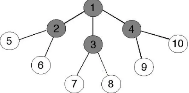
For simplicity, we explain how to calculate P (G4|v1) by an example as shown in Figure 2.1. The vertices colored black are the infected vertices. Suppose v1 is the source, then all possible infecting order i are :
1 = v1 ! v2 ! v3 ! v4 2 = v1 ! v2 ! v4 ! v3 3 = v1 ! v3 ! v2 ! v4
4 = v1 ! v3 ! v4 ! v2 5 = v1 ! v4 ! v3 ! v2 6 = v1 ! v4 ! v2 ! v3
(Note that, if we see v3 as the source then v3 ! v2 ! v1 ! v4 is not a possible infecting order, since there is no edge between v3 and v2.)
Let’s calculate the probability of 1, recall that the infected probability of (t + 1)th vertex is Pt+1(z) = X 1 v2V (Gt) d(v) 2(t 1). Therefore, P ( 1|v1) = 1 3 · 1 4 · 1
5, and also we know that P ( i|v1) = 1 3 · 1 4 · 1 5 for i = 1, 2, 3, 4, 5, 6. In general, we have (2.2) P ( i|v1) = n 1 Y k=1 1 X vi2V (Gk) d(vi) 2(k 1) ,
where Gk is a subgraph of Gnand it represents the infected subgraph at kth time step along with the infecting order i .
For d regular tree,
(2.3) P ( i|v1) = n 1Y k=1
1
dk 2(k 1).
Note that if the rumor has not been spread to leaves of the tree yet, then P ( i|v1) = P ( j|v1) for all i, j 2 S(v, Gn). Now, combining (2.1) and (2.3), then we have
P (Gn|v⇤) = X i2S(v⇤,Gn) P ( i|v⇤) =|S(v⇤, Gn)| · P ( |v⇤) 8 i 2 S(v, Gn) =|S(v⇤, Gn)| · n 1Y k=1 1 dk 2(k 1) _ |S(v⇤, G n)|.
We can now compute each P (G4|vi) by finding out the value |S(vi, Gn)|. Since they are of the same value 1
3·4·5 = 1 60.
Figure 2.1: The example of how to calculate P (G4|v1)
We have:
P (Gn|v1) = 3!· 601
P (Gn|v2) = P (Gn|v3) = P (Gn|v4) = 1· 2! · 601 therefore, by the definition, the ML estimator is v1.
In conclusion, P (Gn|v) is proportional to |S(v, Gn)|, that is, if the rumor didn’t meet the end vertex in the tree yet, then the only fact that a↵ect P (Gn|v) is the number of distinct ways that v can spread the rumor to all vertices in Gn.
Let R(v, Gn) =|S(v, Gn)| be called rumor centrality which is a important infor-mation about the vertex v, we call v the rumor center of Gn if v has the maximum rumor centrality.
2.2
Rumor Centrality R(v, G
n)
Since the P (Gn|v) is proportional to R(v, Gn), we are able to determine which vertex is the ML estimator after calculating all R(vi, Gn) where vi 2 Gn. The following will introduce a formula represents the rumor centrality.
Let Gn be a rooted tree with root vr and suppose G1 = vr, then in G2, the second infected vertex may be any child of vr. There are d(v) vertices in child(v) say ui where i = 1, 2, 3 . . . d(v). So we have: (2.4) R(v, Gn) = (n 1)! tv u1!· t v u2!· . . . · t v ud(v)! · d(v) Y i=1 R(ui, Tuvi).
We can rewrite (2.4) by the recursion from the root vr to all leaves of Gn, then we get a simpler form :
(2.5) R(v, Gn) = n!· Y u2Gn 1 tv u .
Now, consider two adjacent vertices u,v in Gnand a vertex w 2 Gn {u, v}, then we have tv
u = n tuv and tvw = tuw, where tvu is defined in preliminary. By the above two facts, we conclude that
(2.6) P (u|Gn) P (v|Gn) = R(u, Gn) R(v, Gn) = t v u n tu v .
Theorem 2.2.1. [5] Given an n vertices tree Gn. v2 Gn is a rumor center if and only if
tv u n2 for all u2 Gn {v}.
In Gn, we can define the weight [4] of a vertex v in Gn, it is defined as weight(v) = maxu2child(v){tvc} . The vertex of Gn with the minimum weight is called the mass center of Gn. More results on mass center of a tree can be found in [9]. Moreover, the distance centrality [5] of v 2 Gn is defined as D(v, Gn) = Pj2Gnd(v, j). The vertex in Gn with minimum distance centrality is called distance center.
Theorem 2.2.2. Let Gn be defined as in theorem 2.2.1 and v is a vertex in Gn, then the following statements are equivalent:
1. v is a distance center of Gn. [5] 2. v is a rumor center of Gn. [5] 3. v is a mass center of Gn.
Proof. Given Gn be a tree of size n, and v2 Gn.
(1 ) 2) We prove it by contraposition argument, suppose v is not a rumor center, by (2.2.1) there is a branch of v, say Tv
u, with order > n/2 and u is adjacent to v. Now, we need a relationship between Ps2Gnd(v, s) and Ps2Gnd(u, s) described as following. P s2Gnd(v, s) = P s2Gnd(u, s) + (t v u 1) (tuv 1).
We havePs2Gnd(v, s) >Ps2Gnd(u, s), since tv
u > tvu. This implies v is not a distance center.
(2 ) 3) To prove this, we need a fact: If all v’s branches are of order n/2, then v is a mass center. Again, by contraposition argument, suppose v is not a mass center, then there exists a branch of v whose order > n/2, that is, v is not a rumor center by (2.2.1).
(3 ) 1) Suppose v is a mass center, then all it’s branch is of order n/2. This implies v is a rumor center. Let u 2 Gn, if u is adjacent to v, then Ps2Gnd(v, s) < P
s2Gnd(u, s) and we finish the proof. If u is not adjacent to v, then we can partition all vertices in Gn into three sets. The first one is Tvu, the second one is Tuv and the last one contains all vertices not in Tu
v and Tuv say R. Let l denote d(u, v). Now, consider P s2Gnd(v, s) P s2Gnd(u, s) = (Ps2Tu v d(v, s) + P s2Tv ud(v, s) + P s2Rd(v, s)) ( P s2Tu v d(u, s) + P s2Tv ud(u, s) + P s2Rd(u, s)).
(1) |R| + tv u n/2, and tuv > n/2 (2) (Ps2Tv ud(v, s) + P s2Tu v d(v, s)) ( P s2Tv ud(u, s) + P s2Tu v d(u, s)) = l· (t v u tuv) (3) |Ps2Rd(v, s) Ps2Rd(u, s)| l · |R|.
Combine these three properties, we conclude that Ps2Gnd(v, s) Ps2Gnd(u, s) < 0, for any u2 Gn, that is, v is the distance center. ⇤ In [5], it shows that there are at most two rumor centers occur when the maximum size branch of rumor center is of size n/2. In fact, a tree has a either exactly one or exactly two median, see [9] for reference. Note that the definition of median in [8] is similar to distance center.
Now we know how to find the rumor center in a given tree Gn, [5] gave an algorithm called message passing algorithm for calculating each vertex’s rumor centrality R(v, Gn) with time complexity O(n). In chapter 3, we will discuss the correctness of our estimator.
Chapter 3
The Estimator for Rumor Source
in Infinite Trees
In chapter 2, we introduced the idea of “the most possible source”, which we call it a rumor center. When we want to find out the source in Gn, the first vertex we should consider is the rumor center v. So in the following, we will show how to compute the probability P (source = v|Gn).
3.1
The Detection Probability P (source = v
|G
n)
Let G be a tree and Gn is a subtree of G at time n, v is the rumor center of Gn. P (source = v|Gn) is the probability of the event that the rumor center is exactly the rumor source when given Gn. We have,
(3.1) P (source = v|Gn) =
P (Gn|source = v) · P (source = v) P
i2Gn[P (Gn|source = i) · P (source = i)] .
The probability of each vertex to be the source are equal, that is
P (source = i) = P (source = j) 8 i, j 2 Gn, and also we have P (Gn|source = v) _ R(v, Gn).
Thus, (3.2) P (source = v|Gn) = R(v, Gn) P i2GnR(i, Gn) .
With (3.2) we can derive several results about the detection probability.
Theorem 3.1.1. [5] [4] Let G and Gn be defined as above, and v be the rumor center in Gn. Then the detection probability
P (source = v|Gn) 12.
Proof. Given Gnbe the subtree of G with size n, and let v be the rumor center of Gn. Obesrve that, once the rumor has been spread from v to one of its neighbors say u, the number of spreading ways in those remaining vertices is equal to the rumor is originate from u and been spread to v first. So, after the rumor spread from v to u, we contract the edge (u, v) and we view it as a new graph say Gu,v. The new vertex from the contraction called v0. Then we conclude that:
R(v, Gn) =Pu2N(v)R(v0, Gu,v). So, from (3.2) we have
P (source = v|Gn) = P R(v,Gn)
i2GnR(i,Gn)
R(v,Gn)
R(v,Gn)+Pu2N(v)R(v0,Gu,v) 1/2.
⇤ No matter how large the size is or what shape of Gn is, this trivial upper bound won’t change. The following will introduce another bound which is derived from the full d regular tree. Before we introducing this bound, there are two assumptions we need as following:
1. If the size n is fixed, then the full tree has the maximum detection probability. 2. Let Gn be a full tree, then for any k > n the detection probability of Gn is larger than it of Gk.
Let Tc(l, d) denote the d regular complete tree with l levels and v0 is its rumor center. With above assumptions, we have the following result:
Theorem 3.1.2. Let G be a d regular tree, and let Gn and v be defined as in (3.1.1). Let l = blogd 1(n 1d (d 2) + 1)c + 1 and n0 =|Tc(l, d)| where Tc(l, d) is the complete tree with l levels. Then
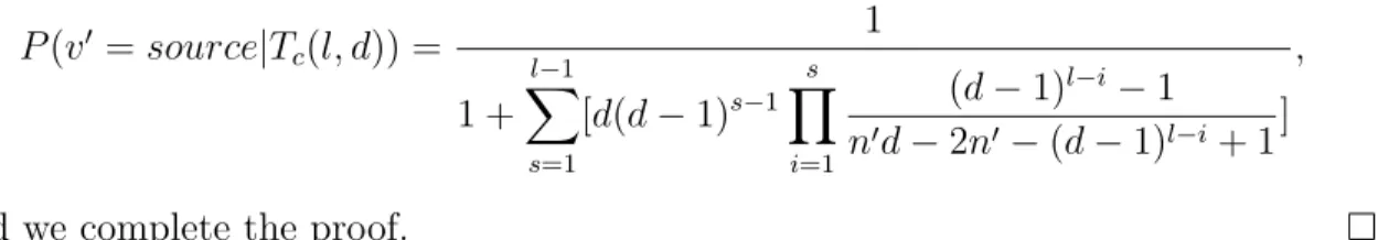
P (source = v|Gn) 1 1 + l 1 X s=1 [d(d 1)s 1 s Y i=1 (d 1)l i 1 n0d 2n0 (d 1)l i+ 1] .
Proof. Let G, Gn and v as defined above, since Tc(l, d) is the maximum size complete tree satisfies |Tc(l, d)| |Gn| and v0 is the rumor center in Tc(l, d). Then from the assumption above, we have :
P (source = v|Gn) P (source = v0|Tc(l, d)) Now, consider P (source = v0|Tc(l, d)) = R(v
0,Tc(l,d))
P
i2Tc(l,d)R(i,Tc(l,d)), our goal is to find out the ratio between v0 and other vertices in Tc(l, d) . By the symmetric structure of the complete tree, we have R(vi, Gn) = R(vj, Gn), if vi and vj are in the same level of the complete tree. Suppose R(v0, T
c(l, d)) = 1, and let vs be the vertex with depth = s , then by property (2.6) we have
(3.3) R(vs 1, Tc(l, d)) : R(vs, Tc(l, d)) = ✓ n0 (d 1) l s 1 (d 2) ◆ : ✓ (d 1)l s 1 (d 2) ◆ ,
for s = 1, 2, 3, ..l 1, where (d 1)(d 2)l s 1 is the number of vertices in Tv0
vs ✓ Tc(l, d). We can rewrite (3.3) as (3.4) R(vs 1, Tc(l, d)) R(vs, Tc(l, d)) = (d 1) l s 1 n0d 2n0 (d 1)l s+ 1.
By the recursive relation in (3.4) and the assumption R(v0, Tc(l, d)) = 1 we have X i2Tc(l,d) R(i, Tc(l, d)) = 1 + l 1 X s=1 [d(d 1)s 1 s Y i=1 (d 1)l i 1 n0d 2n0 (d 1)l i+ 1],
where d(d 1)s 1 is the number of vertex in each level. Thus,
P (v0 = source|T c(l, d)) = 1 1 + l 1 X s=1 [d(d 1)s 1 s Y i=1 (d 1)l i 1 n0d 2n0 (d 1)l i+ 1] ,
and we complete the proof. ⇤ Note that, when n is little enough such that l = 2 then this bound is exactly 1/2 and this bound will decrease as n getting larger. The following is the tendency of the upper bound decreasing as n getting larger.
Figure 3.1: The Tendency of The Upper Bound With di↵erent d
3.2
The Value of P (source = v
|G
n)
In this section, we will compute the detection probability of infinity order d regular tree and show two results which are the same as in [5] but in di↵erent methods.
Theorem 3.2.1. [5] [4] Suppose G is a 2 regular tree, and Gn ✓ G is the infected subtree of G,let v be the rumor center in Gn then
lim
This theorem shows that, the detection probability in a 2 regular tree goes to zero as the infected vertices increase.
Proof. Without loss of generality, suppose the order of the infected subtree is odd and equal to 2t + 1 for some t 2 N.
Given G, G2t+1 as defined above. By theorem 2.2.2, there is a rumor center say v and with R(v, G2t+1) = 2tt . Then, we have
P (source = v|G2t+1) = R(v, G2t+1) P i2G2t+1R(i, G2t+1) = 2t t 2t 0 + 2t 1 + 2t 2 + . . . + 2t 2t = (2t)! t!· t! · 1 22t.
By Stirling Formula, we have lim
t !1
t! p
2⇡ttte t = 1.
Now, consider P (source = v|G2t+1) when t is getting larger. Let Hv
i = {Gi ✓ G| Gi is a 2 regular graph and v is the source of Gi}. So, the detection probability when t is getting larger is :
lim t !1 X G2t+12H2t+1v [P (G2t+1|v) · P (source = v|G2t+1)] = lim t !1P (source = v|G2t+1) = lim t !1 p 4⇡t· (2t)2t· e 2t (p2⇡t· tt· e t)2 · 1 22t = lim t !1 1 p ⇡t = 0. ⇤ The following is going to find out the detection probability in d regular tree with infinity order when d > 2 by the property in Theorem 2.2.1.
Let Ad and Bd be two sets such that Ad={(a1, a2, ..., ad)|0 ai n 2, d X i=1 ai = n 1} and Bd={(b1, b2, ..., bd)|bi 2 N [ {0}, d X i=1 bi = n 1}.
Note that, these two sets are corresponding to the orders of branch’s sizes of a vertex. And if its branch’s size is in Ad then it is the rumor center. We have |Bd| = n 1+d 1d 1 and let Sk = {(s1, s2, ..., sd)|sk > n2, 0 sj < n2, d X i=1 si = n 1}, so |Si| = d+d n 2e 3 d 1 and |Ad| = |Bd| d X k=1 |Sk| = ✓ n + d 2 d 1 ◆ d· ✓ dn 2e + d 3 d 1 ◆ since Si\ Sj = for i6= j.
Given a d regular tree G and let Gn ✓ G, suppose v is the source in Gn with the order of branch’s size (tv
u1, t
v u2, ..., t
v
u3). Recall (2.4), to compute all spreading ways that v can spread to every vertices in Gn we should compute the spreading way in each branch of v first. Suppose u 2 N(v) and now u has the rumor, then there are
1 d 3 tv u Y i=0 ((d 2)(i 1) + 1), for d 4 spreading ways in Tv
u, since there are (d 1) choice when u is going to spread the rumor, and once u spread the rumor to one of its child there are (2d 3) and so on. Note that, when d = 3, 1
d 3 is meaningless so we discuss it separately later in next theorem. Thus, given (tv
u1, t
v u2, ..., t
v
ud) of v, the number of spreading ways is (n 1)! tv u1!· t v u2!· . . . · t v ud(v)! · d Y k=1 [ 1 d 3 tv uk Y i=0 ((d 2)(i 1) + 1)], for d 4.
The corrected detection occurs when rumor center equals to source, so it occurs when the ordered pair of v’s branches belongs to |Ad|. Let Pd(Ct) be the probability of corrected detection at time t in a subtree of d regular tree, then we have
(3.5) Pd(Ct) = (n 1)! X (tv u1,tvu2,...,tvud)2Ad ( d Y k=1 1 d 3 Qtv uk i=0((d 2)(i 1) + 1) tv uk! ) (n 1)! X (tv u1,tvu2,...,tvud)2Bd ( d Y k=1 1 d 3 Qtv uk i=0((d 2)(i 1) + 1) tv uk! ) , for d 4.
Theorem 3.2.2. [5] [4] Let G be a 3 regular tree, then
lim
t !1P3(Ct) = 1 4.
Proof. Let A3 and B3 as defined above. To use (3.5), we should avoid the case when i = 0, that is one of the branch size of v is 0. Let A1
3 be the subset of A3 with at least a zero in (tv u1, t v u2, v u3) and A 2
3 = A3\ A13. Also B13 and B32 are defined repectively. Let zd(i) = (d 2)(i 1) + 1 .Then by (3.5), we have
P3(Ct) = X (tv u1,tvu2,tvu3)2A13 ( 2 Y k=1 Qtv uk i=1(zd(i)) tv uk! ) + X (tv u1,tvu2,tvu3)2A23 ( 3 Y k=1 Qtv uk i=1(zd(i)) tv uk! ) X (tv u1,tvu2,tvu3)2B31 ( 2 Y k=1 Qtv uk i=1(zd(i)) tv uk! ) + X (tv u1,tvu2,tvu3)2B32 ( 3 Y k=1 Qtv uk i=1(zd(i)) tv uk! ) = X (tv u1,tvu2,tvu3)2A13 1 + X (tv u1,tvu2,tvu3)2A23 1 X (tv u1,tvu2,tvu3)2B31 1 + X (tv u1,tvu2,tvu3)2B23 1 = |A1 3| + |A23| |B1 3| + |B32| .
For t is even, we have
|A1 3| + |A23| |B1 3| + |B32| = 6 + t 2 2 3· dt 2e 2 3 1 3 + 3(t 2) + t 22 = n2+ 10n 4t2+ 4t .
|A1 3| + |A23| |B1 3| + |B32| = 3 + t 2 2 3· dt 2e 2 3 1 3 + 3(t 2) + t 22 = n2+ 4n + 3 4t2+ 4t . Thus, lim t !1P3(Ct) = 1 4. ⇤
Theorem 3.2.3. Let G be a d regular tree, then
lim t !1Pd(Ct) = 1 d 2 + (d 2)· d d 2 2d 2d · 1 d 2 d 1 d 2 .
Proof. See the proof in Appendix C.
Corollary 3.2.4. Let G be a d regular tree, then
lim
Chapter 4
Trees with End Vertices
In this chapter, we will discuss about the case that G is a tree not of infinte order. Suppose Gn ✓ G, then there may exists a vertex called end vertex which can only accept the rumor but cannot spread it, since it has only one neighbor.
4.1
The Influence of End Vertices On The
Proba-bility P (v = source
|G
n)
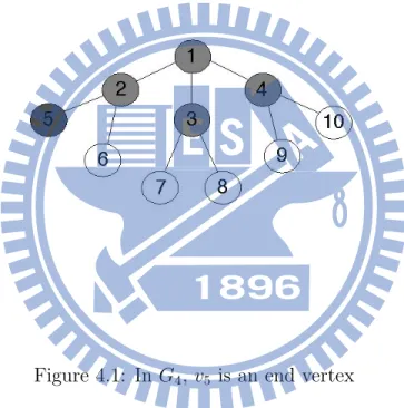
We begin this section with a simple example. Suppose G is a finite order 3 regular tree and G5 ✓ G which is shown in figure 4.1. In G5, it’s easy to find the rumor center is v1. Consider P (G5|v), for the spreading order : v1 ! v2 ! v5 ! v3 ! v4, we have P ( |v1) = 13 · 14 · 13 · 14. Note that if v5 is not the end vertex then P ( |v1) = 13 · 14 · 15 · 16. This shows that the time at when the rumor spread to v5 will has influence on the probability P ( |v1). Now we list out all the spreading ways in the following and sort it according to the position of v5 in each i:
1 : v1 ! v2 ! v5 ! v3 ! v4 2 : v1 ! v2 ! v5 ! v4 ! v3 3 : v1 ! v3 ! v2 ! v5 ! v4 4 : v1 ! v4 ! v2 ! v5 ! v3 5 : v1 ! v2 ! v3 ! v5 ! v4 6 : v1 ! v2 ! v4 ! v5 ! v3 7 : v1 ! v2 ! v3 ! v4 ! v5 8 : v1 ! v2 ! v4 ! v3 ! v5 9 : v1 ! v3 ! v2 ! v4 ! v5 10: v1 ! v3 ! v4 ! v2 ! v5
11 : v1 ! v4 ! v2 ! v3 ! v5 12 : v1 ! v4 ! v3 ! v2 ! v5.
According to the above, we conclude that P ( 1|v) = P ( 2|v) = 1441 , P ( 3|v) = P ( 4|v) = P ( 5|v) = P ( 6|v) = 2401 , and P ( 7|v) = P ( 8|v) = P ( 9|v) = P ( 10|v) = P ( 11|v) = P ( 12|v) = 3601 . So, P (G5|v1) = 72034. We also have P (G5|v4) = P (G5|v3) =
7
720 by symmetric, and P (G5|v2) = 40
720. Note that although v1 is the rumor center we have P (G5|v1) < P (G5|v2). So we will guess v2 as the source, the example shows that the earlier the end vertex appears in i the larger P ( i|v) it will be.
Figure 4.1: In G4, v5 is an end vertex
From this example we conclude that in a finite network, not only the spreading way has influence on the probability of being a candidate of the source but also the distance from the end vertex. Suppose there are two adjacency vertices say v1and v2 in a finite tree Gn which has an end vertex ve, with R(v1, Gn) > R(v2, Gn) and d(v2, ve) = m. If v1 lies on the path from v2 to ve, then we have P (Gn|v1) > P (Gn|v2). Let ⌦kv1 be the set of all permutation (each permutation represents a spreading way) that started from v1 and ve is the (k + 1)th element in the permutation, then |⌦kv1| |⌦
k
v2|. Since for any k 2 N, there are k m choice before the rumor be spread to ve for v1, but
there are only k m 1 choice for v2, in addition, if v2 wants to spread the rumor to ve, the rumor must pass through v1, conversely then not. From the observation, we have the following theorem.
Theorem 4.1.1. Let G be a tree with finite order and Gn ✓ G is a subtree of G with an end vertex ve 2 Gn, then the vertex v⇤ with maximum probability P (Gn|v) is located on the path from rumor center to ve.
Figure 4.2: Gn with an end vertex vd+1
Proof. Let G, Gn as defined above. vr is the rumor center in Gn and ve is the end vertex in Gn. Suppose d(vr, ve) = d. Then, the path P from vr to ve is shown in figure 4.2, where v1 = vr and vd+1 = ve. Define Di ={ v 2 Gn| the path from v to ve contains vi }. Given i = 1, 2, ..., d, let v 2 Di, then we have R(v, Gn) R(vi, Gn) (Suppose not, then v1 is not the rumor center, we get a contradiction.) So, each vertex in Di has less spreading ways than vi and farther from ve than vi does. By the
observation above, we conclude that P (Gn|vi) P (Gn|v). So, the vertex with the maximum probability to spreading the rumor all over Gn is located on the path from
v1 to ve. ⇤
Note that, if all leaves are end vertices, that is Gn = G, then the probability P (Gn|v) of each vertex in Gn is n1, since any vertex is able to spread the rumor to all vertices in G in n step when Gn= G.
4.2
Computing P (G
n|v)
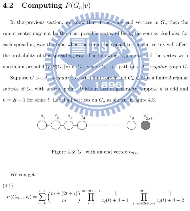
In the previous section, we know that if there are end vertices in Gn then the rumor center may not be the most possible vertex of being the source. And also for each spreading way the time when the rumor be spread to the end vertex will a↵ect the probability of this spreading way. The following is going to find the vertex with maximum probability P (Gn|v) in Gn, where Gn is a path on a d regular graph G. Suppose G is a d regular tree with finite order and Gn ⇢ G is a finite 2-regular subtree of Gn with an end point. Without loss of generality, suppose n is odd and n = 2t + 1 for some t. Label all vertices on Gn as shown in figure 4.3.
Figure 4.3: Gn with an end vertex v2t+1
We can get (4.1) P (G2t+1|vi) = i 1 X m=0 ✓ m + (2t + i) m ◆m+2t+1 iY l=1 1 zd(l) + d 1· 2t 1Y l=m+2t+1 i 1 zd(l) + d 2
for i = 1, 2, ..., 2t. And P (G2t+1|v2t+1) = 2t Y l=1 1 zd(l) .
We can find that, to compute all spreading way of vi is equal to find all ways from i to the lower right corner in the figure 4.4.
In (4.1) m = 0 means i goes right to the end and then goes down to the end, that is, vi spread the rumor straight to the end vertex and then spread to the rest of vertices. So m is the parameter related to the time when the rumor meets the end vertex. And the left Q is the probability of this sprading way when the rumor meet the end vertex and the right one is the probability after the rumor met the end vertex.
From (4.1) we can use computer to compute P (G2t+1|vi) for all i, the following is the numerical result for d = 2, 3 and n = 41, where d for d regular and n = 2· t + 1 is the size of Gn. In these figures, the x axis is the node vi where i = 1, 2, ..., n, and the y axis is the probability P (vi = source|Gn). See more figures in appendix.
Figure 4.4: d=2,n=41 Figure 4.5: d=3,n=41
Finally we will introduce how to compute the P (Gn|v) for each vertex in Gnwhere Gn is general subgraph of G with an end vertex, G is a finite d regular tree. When we compute the probability of a spreading way we should compute the probability before the rumor meets the end vertex and after the rumor meets the end vertex separately just as the case above.
Let G be a finite d regular tree and Gn ✓ G is a subtree of G of order n with an end vertex ve. Given v 2 Gnand v 6= ve. Let mv(t) be the number of permutation started from v and ve is located on the (t + 1)th element in the permutation. Then we have (4.2) P (Gn|v) = n 1 X t=d(ve,v) mv(t) t Y i=1 1 d + (i 1)(d 2) · n 2 Y i=t 1 d + (i 1)(d 2) 1
The di↵erence between (4.1) and (4.2) is that mv(t) is easy to compute moreover we can write a formula for it when Gn is a path, but in general tree mv(t) is unknown. To compute mv(t) is a hard problem, it is equal to list out all permutation started from v.
4.3
Conclusion and Future Work
In the infinite case, we can compute all d2 N, by counting the number of increas-ing trees in a d regular tree. In the finite case, we provided a theorem indicate the “most possible source” lies on the path from rumor center to the end vertex. To compute mv(t) for all possible t and for all v lies on the path, we have two algorithms. One is by brute force, that is, to list out all possible spreading ways from v and then count mv(t) for each t. Another one is a two-step algorithm, see details in appendix B. The second one is more complicated. Since mv(t) is related to the shape or struc-ture of Gn, it’s hard to derive a general formula. The future study would be finding a efficient method to compute mv(t).
Appendix A
More Figures on Detection
Probability
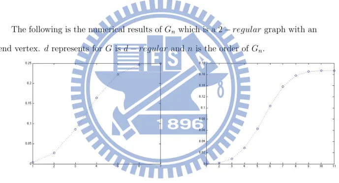
The following is the numerical results of Gn which is a 2 regular graph with an end vertex. d represents for G is d regular and n is the order of Gn.
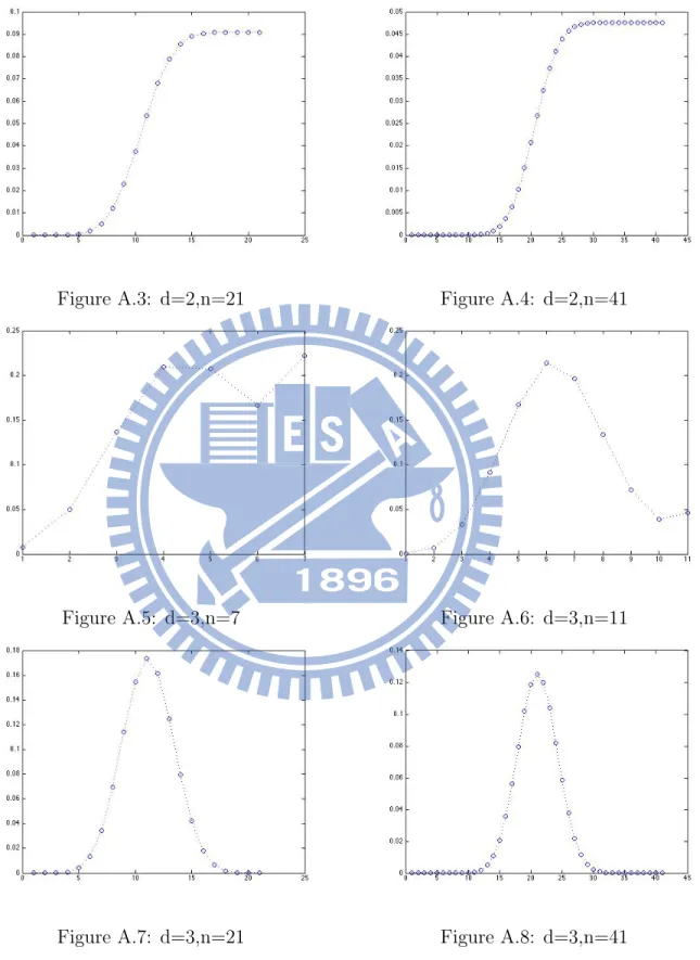
Figure A.3: d=2,n=21 Figure A.4: d=2,n=41
Figure A.5: d=3,n=7 Figure A.6: d=3,n=11
Figure A.9: d=5,n=7 Figure A.10: d=5,n=11
Figure A.11: d=5,n=21 Figure A.12: d=5,n=41
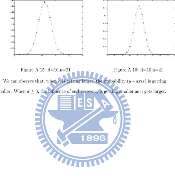
Figure A.15: d=10,n=21 Figure A.16: d=10,n=41
We can observe that, when n is getting larger, the probability (y axis) is getting smaller. When d 3, the influence of end vertex vn is getting smaller as n gets larger.
Appendix B
Two-Steps Method for Computing
m
v
(t)
Let G be a tree, and Gn is a subtree of order n (n subtree for short). P is the path from root v to the end vertex ve, and suppose d(v, ve) = d. Let mv(t) be the number of permutations started from v and ve is located on the (t + 1)th element in these permutations. In [6], it provided an algorithm to enumerate the number of n subtree in a tree. We just need a part of its algorithm, which is to find the family of subtrees whose root are v.
First, we should contract all vertices lie on the path P except ve, then we get a new tree G0 and v0 represents those contracted vertices. Now we can apply the algorithm to find a (t d) subtree with root v0. For each (t d) subtree in G0, we can find the number of spreading ways started from v0 by using (2.5). The (t + 1)th vertex must be ve.
In the second step, after the rumor spread to ve, we contract all these t + 1 vertices. We get a new tree G00 from G0 and a new vertex v00 represents those vertices contracted. We can use (2.5) again to find out the number of spreading ways. After combining step one and step two, we can find out mv(t). See more details about the algorithm for listing all n subtree in a tree in [6].
Appendix C
Proof of Theorem 3.2.3
We consider rumor spreading on d-regular graphs. First, we fix some notations. Let ˜Tndenote the tree after the rumor has spread to n nodes. We give the vertices labels from the set {1, 2, . . . , n} according to the first time a vertex learns the rumor. Thus, the vertex with label 1 is the source and it is the only node with outdegree d whereas all other nodes have outdegree d 1 (if ˜Tn is drawn as a rooted tree in the usual way).
Next, note that the d subtrees of the source are d 1-ary increasing trees (increas-ing trees are labeled trees with label sequences from the root to any leaf increas(increas-ing). Set
Tn= number of (d 1)-ary increasing trees, T (z) = X n 1
Tn zn n!. It is easy to derive that
(3.1) T (z) = 1 + (1 (d 2)z) 1/(d 2).
Next, set
˜
Tn = number of possible ˜Tn and T (z) =˜ X n 1 2 ˜Tn zn n!. Then, (3.2) ˜Tn= 1 2 n Y i=1 [2 + (d 2)(i 1)] and T (z) =˜ 1 + (1 (d 2)z) 2/(d 2)
We are interested in Cn, the event that the source of ˜Tn is the rumor center. We have,
P (Cn) = 1 dP (size of one subtree of the source of ˜Tn n/2).
We fix one subtree of the source of ˜Tn say tv1 and denote by I its size. Let ji represent the size of the i th subtree of ˜Tn. Obviously,
P (I = j) = 1 ˜ Tn X j+j2+j3+...+jd=n 1 ✓ n 1 j, j2, j3, . . . , jd ◆ TjTj2Tj3. . . Tjd = (n 1)!Tj j! ˜Tn X j2+j3+...+jd=n 1 j Tj2 j2! Tj3 j3! . . .Tjd jd! = (n 1)!Tj j! ˜Tn [zn 1 j](1 + T (z))d 1 = (n 1)!Tj j! ˜Tn [zn 1 j](1 (d 2)z) d 1d 2 = (n 1)!Tj j! ˜Tn (d 2)n 1 j[zn 1 j](1 z) d 1d 2 = (n 1)!Tj j! ˜Tn (d 2)n 1 j(n 1 j) 1 d 2 (d 1 d 2) . (3.3)
In the sequel, we need the following standard lemma from analytic combinatorics.
Theorem C.0.1 (Theorem VI.1 in [2]). For ↵2 C \ Z0 set f (z) := (1 z) ↵. Then, as n! 1, [zn]f (z)⇠ n ↵ 1 (↵) 1 + 1 X k=1 ek(↵) nk ! ,
where ek(↵) is a polynomial of degree 2k.
Asymptotics. We now turn to asymptotics. The following computation is based on n! 1.
First, applying Theorem C.0.1 to (3.1) gives
Tn⇠
n!· n2 dd 1
(d 11 ) (d 1)
n (n
Similarly, applying Theorem C.0.1 to (3.2) yields ˜ Tn⇠ n!· n4 dd 2 2 (d 22 )(d 2) n (n ! 1). By theorem 2.2.1, we need to compute
X n/2jn 1
P (I = j),
where P (I = j) is given by (3.3). Therefore, we again use Theorem C.0.1 and the expansions for Tn and ˜Tn from above. This gives
X n/2jn 1 P (I = j) ⇠ (n ˜ 1)! Tn X n/2jn 1 Tj j! (d 1 d 2) (d 2)n 1 j(n 1 j)d 21 ⇠ (n 1)!· 2 ( 2 d 2) n!· n4 dd 2(d 2)n X n/2jn 1 j!·j3 dd 2 ( 1 d 2)(d 2) j j! (d 1 d 2) (d 2)n 1 j(n 1 j)d 21 ⇠ 2 2 d 2 (d 2)· nd 22 ( 1 d 2) ( d 1 d 2) X n/2jn 1 jd 21 1(n 1 j)d 21 ⇠ 2 2 d 2 (d 2)· nd 22 ( 1 d 2) ( d 1 d 2) · nd 22 1 X n/2jn 1 ✓ j n ◆ 1 d 2 1✓n 1 j n ◆ 1 d 2 ⇠ 2 ( 2 d 2) (d 2) ( 1 d 2) ( d 1 d 2) Z 1 1/2 xd 21 1(1 x) 1 d 2dx (n ! 1). Lemma 1. Z 1 1/2 xc 1(1 x)cdx = 1 2 ✓ B(c, c + 1) 1 c· 22c ◆ Proof. Z 1 0 xc 1(1 x)cdx = Z 1/2 0 xc 1(1 x)cdx + Z 1 1/2 xc 1(1 x)cdx
Now, consider the right part R1/21 xc 1(1 x)cdx, and name it R (the left part is L). By integration by part we have
R = 1
c(1 x) cxc 1
So L = R1 0 x c 1(1 x)cdx + 1 c·22c 2 = B(c, c + 1) +c·212c 2 , and R = 1 2 ✓ B(c, c + 1) 1 c· 22c ◆ . ⇤ Finally, combining everything yields for the detection probability of the source in d-regular trees is the following limit
lim t !1Pd(Ct) = 1 d· X n/2jn 1 P (I = j) = 1 d 2 + (d 2)· d d 2 2d 2d · 1 d 2 d 1 d 2
References
[1] Thomas H. Cormen, Charles E. Leiserson, Ronald L. Rivest and Cli↵ord Stein, Sedgewick, Introduction to Algorithm 3th ed, The MIT Press, Cambridge, Mas-sachusetts London, England 2009.
[2] Philippe Flajolet, Robert Sedgewick, Analytic Combinatorics, Cambridge Uni-versity Press, 2009.
[3] A. Ganesh, L. Massoulie, and D. Towsley, “The e↵ect of network topology on the spread of epidemics”, Proc. 24th Annual Joint Conference of the IEEE Computer and Communications Societies (INFOCOM), vol. 2, pp. 1455-1466, March 2005.
[4] Zi-Hui Lee, “A Mathematical Model for Finding the Culprit Who Spreads Ru-mors”, A Thesis Submitted to Department of Applied Mathematics College of Science National Chiao Tung University in Partial Fulfillment of the Require-ments for the degree of Master in Applied Mathematics, June 2012.
[5] D. Shah and T. Zaman, “Rumors in a Network: Whos’s the Culprit?”, IEEE Transactions on information Theory, vol. 57, pp. 5163-5181, August 2011.
[6] Kunihiro Wasa, Yusaku Kaneta, Takeaki Uno, and Hiroki Arimura, “Constant Time Enumeration of Bounded-Size Subtrees in Trees and Its Application”, IST, Hokkaido University, Sapporo, Japan.
[7] Yang Wang, Deepayan Chakrabarti, Chenxi Wang, Christos Faloutsos, “Epi-demic Spreading in Real Networks: An Eigenvalue Viewpoint”, Carnegie Mellon University.
[8] D.B. West, Introduction to Graph Theory , second edition, Prentice Hall, Upper Saddle River, New Jersy, 2011.
[9] Bohdan Zelinka,“Medians and Peripherians of Trees’, Archivum Mathematicum, Vol. 4 (1968), No.2, 87–95.