在未標號圖形資料中高效率的圖形探勘演算法

國

立

交

通

大

學

資訊科學與工程研究所

碩

士

論

文

在未標號圖形資料中高效率的圖形探勘演算法

An Efficient Algorithm for Mining Frequent Unlabeled Graphs

研 究 生：李 銘

指導教授：李素瑛 教授

在未標號圖形資料中高效率的圖形探勘演算法

An Efficient Algorithm for Mining Frequent Unlabeled Graphs

研 究 生：李 銘 Student：Ming Lee

指導教授：李素瑛 Advisor：Suh-Yin Lee

國 立 交 通 大 學

資 訊 科 學 與 工 程 研 究 所

碩 士 論 文

A Thesis

Submitted to Institute of Computer Science and Engineering College of Computer Science

National Chiao Tung University in partial Fulfillment of the Requirements

for the Degree of Master

in

Computer Science

June 2010

Hsinchu, Taiwan, Republic of China

在未標號圖形資料中高效率的圖形探勘演算法

研究生：李銘

指導教授：李素瑛

國立交通大學資訊科學與工程研究所

摘要

近年來頻繁樣式探勘由頻繁項目集探勘及循序樣式探勘逐漸發展至探勘更 具結構性之資料，例如樹、絡及圖形等資料。圖形可用於表示許多複雜的資料及 資料間的關係，因此被廣泛應用於許多領域，如化學資訊學、生物資訊學及網路 探索等等。由於圖形資料的高複雜度，其子圖的個數呈指數成長，如何有效率的 探勘大型圖形樣式是一項重大的挑戰。在過去十年間，發展出了許多圖形探勘演 算法，我們研究目前已知最好的演算法 gSpan ，希望能更進一步改善其效率。 gSpan 採用 right-most 延伸法來產生候選圖形，與傳統方法比較，其產生之重 覆的候選圖形數目顯著減少。但由於 right-most 延伸法原本是用於有根樹的探 勘演算法，以此為基礎用於圖形探勘，仍會產生許多重覆的候選圖形。此情況造 成 gSpan 的效能降低，尤其在針對標記種類較少、或甚至未標號的圖形做處理 時，效能的降低更為顯著。因此我們修正此延伸法以進一步減少候選圖形個數， 並將之用於未標號圖形資料中。我們對合成資料以及實際之化學化合資料進行實 驗，驗證了所提演算法之正確性，並且有效的減少了候選圖形的個數。

An Efficient Algorithm for Mining Frequent Unlabeled Graphs

Student: Ming Lee Advisor: Suh-Yin Lee

Institute of Computer Science and Information Engineering

National Chiao-Tung University

Abstract

In recent years, academic research on pattern discovery progressed from mining

frequent itemsets and sequences to mining structured patterns including trees, lattices,

and graphs. Among them, graphs serve as a general model to represent data and have

consequently been widely and extensively used in many domains like

cheminformatics, bioinformatics, web exploration, etc. However, mining large graph

patterns effectively and efficiently is challenging due to the presence of an

exponential number of frequent subgraphs and the complexity of graph data. In

response to the dilemma, several graph miners, such as gSpan, have been published in

the last decade and all of these newly developed graph miners work on undirected

labeled simple graph. By examining the state-of-the-art pattern growth algorithm

gSpan, which uses a right-most extension method, we learn that it dramatically

reduces the number of candidate graphs, compared with traditional join method.

generates many duplicate graphs when being applied to a free graph. This problem

causes remarkable performance degradation when the graphs are denser and with

fewer labels available, especially when the graphs are unlabeled. We propose a

modified extension method to further decrease the number of duplicate graphs, and

apply it to unlabeled graph datasets, hoping to make gSpan an even better miner than

it already is. We present the results on mining both synthetic datasets and a chemical

誌謝

首先，最感謝的是指導教授李素瑛老師。多年來，老師在研究上、生活上都 非常有耐心的給我許多指導，使我有很大的收獲。也感謝老師在我犯錯時的諸多 包容。 感謝沈錳坤教授和彭文志教授撥冗擔任我的口試委員，並提供許多寶貴的建 議，充實了本論文。 感謝資訊系統實驗室的所有成員：渏紋、健鵬、以錚學長及育君、蕙媜學姊 在研究及生活上的幫助，也感謝鵬屹、季強、維晉同學，與誠毅、書華、憲智學 弟，研究生活因你們多了許多歡笑與回憶。感謝我的高中好友晏慶在生活上的照 顧與協助。也感謝我的研究所同學瀚萱、本然及大學好友承翰及雋永，與我分享 生活中的種種精彩事物。更要感謝好友靖賢，在人生方向及論文寫作上給我許多 建議。 感謝我的家人，總是給予我關懷與支持，在我遇到困難時總是想盡辦法幫助 我，有了你們的辛苦與支持，才有今日的我。 要感謝的人很多，在此向所有曾幫助關心過我的人，致上最真切的謝意。 僅以此論文獻給所有關心我的人。

Table of Contents

Chinese Abstract ... i English Abstract ... ii Acknowledgement ... iv Table of Contents ... v List of Figures ... vi

List of Tables ... vii

Chapter 1 Introduction ... 1

Chapter 2 Related Works ... 7

2.1 The Apriori-Based Approach ... 7

2.2 The Pattern-Growth Approach ... 10

Chapter 3 Problem Definitions ... 14

Chapter 4 The Graph Mining Algorithm ... 17

4.1 Lexicographic Order ... 19 4.1.1 DFS Subscripting ... 20 4.1.2 DFS Code ... 21 4.1.3 DFS Lexicographic Order ... 24 4.2 Right-Most Extension ... 26 4.3 gSpan ... 28

4.4 The Proposed Enumeration Method ... 31

Chapter 5 Experimental Results ... 34

Chapter 6 Conclusion and Future Works ... 38

List of Figures

Fig. 1-1 A sample graph data set of chemical structures ... 2

Fig. 1-2 Free extension ... 4

Fig. 1-3 Right-most extension ... 5

Fig. 1-4 Three isomorphic graphs ... 5

Fig. 2-1 AGM: Two graphs joined by two paths ... 8

Fig. 2-2 FSG: Two graphs and their potential candidates ... 9

Fig. 2-3 Runtime of the four algorithms ... 13

Fig. 2-4 Memory Usage of the four algorithms ... 13

Fig. 3-1 A labeled graph ... 14

Fig. 3-2 An example of subgraph isomorphism ... 16

Fig. 3-3 An Example of the supports of graphs ... 16

Fig. 4-1 A naïve graph mining algorithm ... 18

Fig. 4-2 Four different ways to generate g ... 19

Fig. 4-3 DFS subscripting ... 21

Fig. 4-4 An example of edge order ... 23

Fig. 4-5 The graphs extended from the graph in Fig. 4-3(b) ... 27

Fig. 4-6 An example of non-minimum DFS code ... 28

Fig. 4-7 A DFS code tree ... 29

Fig. 4-8 The pseudo code of gSpan [28] ... 29

Fig. 4-9 The function isMinimum ... 30

Fig. 4-10 The search space of gSpan ... 31

Fig. 4-11 A right-most extension ... 32

Fig. 5-1 Number of candidates (synthetic dataset) ... 36

List of Tables

Table 4-1 DFS codes for the graphs in Fig.4-3(b)-(d) ... 24 Table 5-1 Synthetic dataset parameters ... 35

Chapter 1

Introduction

Over the past few decades, frequent pattern mining has been an active and

prevalent research topic in data mining with many techniques. These techniques were

developed for the purpose of mining association rules [1], frequent itemsets [6, 7, 13,

27], sequential patterns [2, 17, 19], trees [3, 26], as well as graphs [10, 14, 15, 16, 28,

30].

Among all these data types, graphs, as a general data structure, can be used to

model more complicated relations among data. For instance, the chemical structure of

a given chemical compound can be modeled by an undirected labeled graph in which

each vertex corresponds to an atom and each edge corresponds to a chemical bond

between atoms. In electronic transactions, the vertices of graphs represent the account

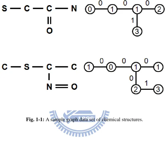
owners and the edges of graphs indicate the occurrence of payments. Fig.1-1 shows a

sample set of chemical structures and their related graphs. Graphs have been used in

chemical informatics [4, 5, 22, 23], computer vision [25], video indexing [20],

machine learning [14], and text retrieval [12], etc.

The frequent subgraph mining problem is to find frequent subgraphs over a

no less than a user-specified threshold.

Fig. 1-1: A sample graph data set of chemical structures.

The kernel of frequent subgraph mining lies in thesubgraph isomorphism test. A

number of isomorphism test algorithms were developed in the past three decades,

such as Backtracking proposed by J. R. Ullmann[24] and Nauty proposed by B. D.

McKay [18]. They solve the graph isomorphism problem by calculating the canonical

labels [35] of graphs. The canonical label is one of the most generic and important

graph invariants. The Nauty algorithm is known to be one of the fastest algorithm for

isomorphism problem of a general graph has been proved to be NP-complete [31].

Therefore,no polynomial algorithm is able to solve it. The time-consuming process of

the isomorphism test leads to the fact that thecandidate test cannot be done with ease.

Early implementations of graph miner generate huge candidate set which contains a

large number of duplicate graphs. For each candidate graph, lots of isomorphism tests

need to be performed to determine whether it is a duplicate graph. As a result, testing

of false candidates degrades the performance to a certain degree.

Recently, Yan and Han [28] proposed a pattern growth based graph pattern

mining algorithm, gSpan, which was inspired by PrefixSpan [19], TreeMinerV [26],

and FREQT [3]. gSpan adopts a canonical labeling system, i.e. DFS (depth-first

search) lexicographic order. Each graph is assigned a unique minimum DFS code. In

the mining process, a graph is a duplicate if and only if its DFS code is not minimum.

gSpan detects duplicate graphs by calculating their minimum DFS codes. gSpan also

adopts a right-most extension strategy, which generates fewer candidate graphs. The

right-most extension grows a graph pattern by adding a new edge to the vertices on

the right-most path, but not to an arbitrary vertex. A right-most path of a graph is the

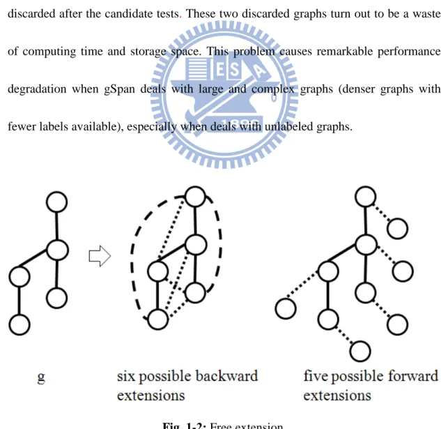
path from the first vertex to the latest added vertex. Fig. 1-2 shows a result of

extending g which adds new edges to arbitrary positions. Fig. 1-3 shows all the

right-most path of g. The dotted line show the new edges added to g. In this example,

the number of candidate graphs is decreased from eleven to four. Consequently, a

huge number of isomorphism tests are avoided. As a result, the storage cost is reduced

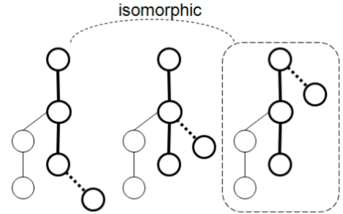
and the performance is improved significantly. However, gSpan generates some

duplicate graphs since the right-most extension method is originally used for rooted

tree mining. For example, Fig.1-4 shows three isomorphic graphs. In the mining

process of gSpan, all of these three graphs will be generated, but two of them will be

discarded after the candidate tests. These two discarded graphs turn out to be a waste of computing time and storage space. This problem causes remarkable performance

degradation when gSpan deals with large and complex graphs (denser graphs with

fewer labels available), especially when deals with unlabeled graphs.

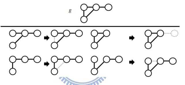
Fig. 1-3 Right-most extension

Fig. 1-4: Three isomorphic graphs.

In mining the rooted tree, the right-most extension method does not generate any

duplicate while in mining the free graph, it does. Therefore, in Fig. 1-3, we can see

right-most extension method to make it more suitable for general graphs, which

prevents some duplicate graphs from generating. We apply this method to unlabeled

graph datasets to evaluate the percentage of decreased duplicate graphs.

The rest of this thesis is organized as follows. Chapter 2 focuses on related works.

Chapter 3 provides the details of problem definitions. Chapter 4 introduces the

algorithm of gSpan and formulates our graph mining algorithm. Chapter 5 gives the

experimental results. Chapter 6 summarizes the entire work and proposes the future

Chapter 2

Related Works

Recent studies have developed several graph-based data mining methods. The

pioneering work appeared in around 1994, when Holder et al. [14] proposed

SUBDUE to carry out approximate subgraph pattern discovery based on minimum

description length and background knowledge. Since SUBDUE uses a

computationally-constrained beam search, it cannot discover the complete set of

frequent patterns. The first system to try complete search for the wider class of

frequent subgraph named WARMR was later proposed by Dehaspe et al. [32] in 1998.

It applied inductive logic programming to the prediction of chemical carcinogenicity

by mining subgraphs. Besides these studies, recent approaches of graph-based data

mining can be categorized into two groups, an Apriori-based approach and a

pattern-growth approach. In the following a brief recount of these approaches will be

introduced.

2.1 The Apriori-based Approach

search starts with graphs of small size, and proceeds in a bottom-up manner. At each iteration, the size of subgraphs is increased by one. These new subgraphs are first generated by joining two similar frequent subgraphs that were discovered already. Afterwards, the occurrence of the new graphs is checked. Typical Apriori-based frequent subgraph mining algorithms include AGM by Inokuchi et al. [15], and FSG by Kuramochi and Karypis [16].

AGM (Apriori-based Graph Mining) adopts a vertex-based candidate generation

strategy that increases the subgraph size by one vertex at each iteration. Two size-k

frequent graphs are joined only when the two graphs have the same size-(k-1)

subgraph. Fig. 2-1 shows the two subgraphs joined by two paths. AGM actually forms

two candidates because it is impossible to determine whether there is an edge

connecting the additional two vertices before the generation.

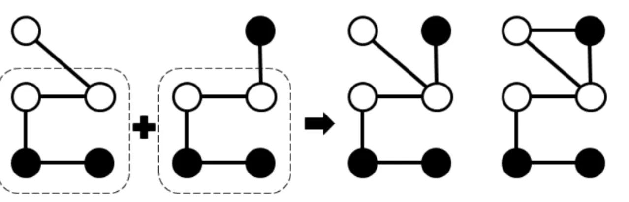
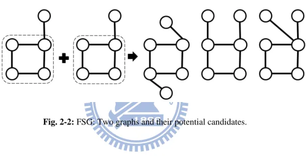
FSG (Frequent SubGraph discovery) uses an edge-based candidate generation

method that extends the subgraph by one edge at each iteration. Two size-k graphs are

joined if and only if they share the same subgraph having k-1 edges. An example of

the candidate generation of FSG is shown in Fig. 2-2.

Fig. 2-2: FSG: Two graphs and their potential candidates.

Comparatively speaking, AGM finds all frequent induced subgraphs in a graph

database while FSG finds all frequent connected subgraphs in a graph database. These

two pioneering Apriori-based frequent subgraph mining algorithms at the time when

they were proposed, however, both bear three problems, which are later modified and

fixed by newer and better ways. These problems include: (1) Huge candidate

generation. (2) Multiple scans of database. (3) Difficulties in mining long patterns.

pattern-growth strategy to avoid these problems.

2.2 The Pattern-growth Approach

Pattern-growth-based graph mining algorithms include gSpan by Yan and Han.

[29], MoFa by Borgelt et al. [33], FFSM by J. Huan et al. [34], and Gaston by Nijssen

et al. [30] These algorithms are inspired by the sequence mining algorithm,

PrefixSpan [19], and the tree mining algorithms, TreeMinerV [26], FREQT [3]. All of

them use a depth-first search for finding candidate frequent subgraphs.

The pattern-growth-based mining algorithms extend a frequent graph by adding a new edge in every possible position. A problem with the edge extension is that the same graph can be discovered many times.

MoFa (Molecule Fragment Miner) uses an embedding list to store the

information of vertices and the information of edges. Extension is restricted to those

graphs, which actually appear in the database. Isomorphism tests in the database can

cheaply be done by testing whether an embedding can be refined in the same way.

MoFa uses a graph local-numbering scheme to reduce the number of candidates

generated from a graph. MoFa sorts the vertices of a graph according to the sequence

may only occur at v or at vertices bigger than v. Moreover, all extensions that grow

from the same vertex v are ordered according to increasing vertex and edge labels.

Although this local ordering helps, MoFa still generates many isomorphic graphs and

then uses standard isomorphism testing to prune duplicates.

gSpan (graph-based Substructure pattern mining) uses a canonical representation

for graphs, called DFS code. A DFS traversal of a graph defines an order in which the

edges are visited. The concatenation of edge representations in that order is the

graph’s DFS code. Candidate generation is restricted by gSpan with the following rule:

graphs can only be extended at vertices that lie on the rightmost path. This restriction

reduces the generation of isomorphic candidates, but it cannot fully prevent duplicates

from generating. Therefore, gSpan computes the canonical DFS-code for each graph.

Graphs with non-minimum DFS code can be pruned. Since instead of embeddings,

gSpan only stores appearance lists for each graph, subgraph isomorphism testing must

be done on all graphs in these appearance lists.

FFSM (Fast Fragment Subgraph Mining) represents graphs as triangle matrices

(vertex labels on the diagonal, edge labels on the other positions). The matrix code is

the concatenation of all its entries, left to right and row by row. Based on

lexicographic ordering, isomorphic graphs have the same canonical code, CAM

candidates. The extension has a restriction: a new edge-vertex pair can only be added

to the last vertex of a CAM. After candidate generation, FFSM permutes matrix line

to check whether a generated matrix is canonical. If not, it can be pruned. FFSM

stores embeddings to avoid explicit subgraph isomorphism testing. However, FFSM

only stores the matching vertices, edges are ignored. This helps speeding up the

extension operations since the embedding lists of new graphs can be calculated by set

operations on the vertices.

Gaston (Graph/sequence/tree extraction) considers graphs that are paths or trees

first, and by only proceeding to general graphs with cycles at the end, a large fraction

of the work can be done efficiently, since there are efficient ways to enumerate paths

and trees. Only in the last phase, Gaston faces the NP-completeness of the subgraph

isomorphism problem. Gaston defines a global order on cycle-closing edges and only

generates those cycles that are larger than the last one. A graph isomorphism test is

then performed on those general graphs with cycles for finding duplicates.

A comparison among these four algorithms of both runtime and memory usage

has been done by M. Worlein et al. [38]. The comparison results are shown in Fig. 2-3

and Fig. 2-4. Considering both the runtime and the memory usage, gSpan has the best

Chapter 3

Problem Definitions

In this chapter, some basic background knowledge with respect to graphs will be

described. And then the frequent subgraph mining problem will be defined.

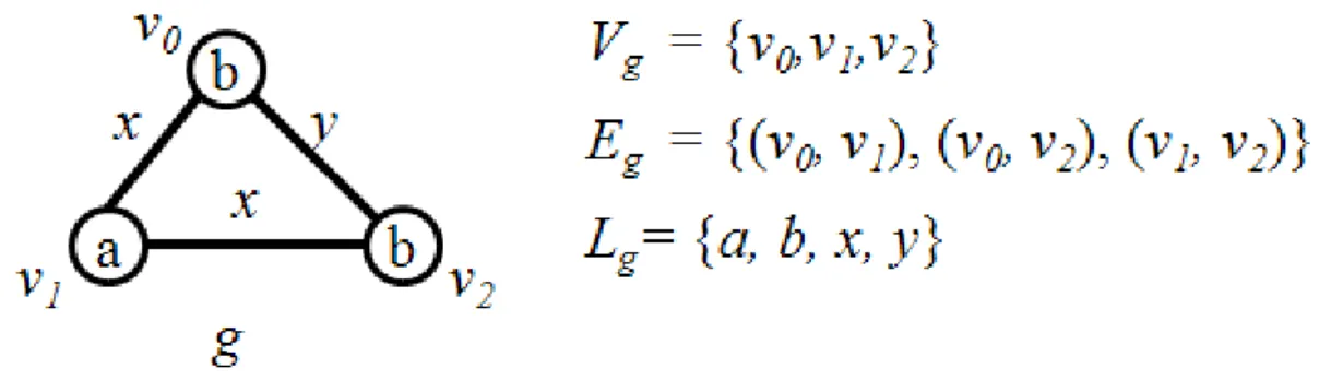
Definition 1 (Labeled Graph) A labeled graph can be represented by a six-tuple,

G = (V, E, L, lv, le ), where

V is a set of vertices, E ⊆ V × V is a set of edges, L is a set of labels,

lv : V → L, l is a function assigning labels to the vertices,

le : E → L, l is a function assigning labels to the edges.

In the rest of this thesis, we denote the sets and the functions corresponding to a graph g as Vg, Eg, Lg, lvg,and leg. Fig. 3-1 shows an example of a labeled graph g. In

this example, lvg(v0) = b, lvg(v1) = a, lvg(v2) = b, leg(v0, v1) = x, leg(v0, v2) = y, and

leg(v1, v2) = x.

Definition 2 (Subgraph) Given a pair of labeled graphs G = (V, E, L, lv, le) and G’ =

(V’, E’, L’, lv’, le’), G is a subgraph of G’ if and only if

V ⊆ V’,

∀ u ∈ V, lv(u) = l’v(u),

E ⊆ E’,

∀(u,v) ∈ E, le(u,v) = l’e(u,v).

Definition 3 (Isomorphism) A labeled graph G = (V, E, L, lv, le) is isomorphic to

another graph G’ = (V’, E’, L’, lv’, le’) if and only if there exists a bijective function

f : V → V’, such that ∀ u ∈ V, lv(u) = lv’(f(u)),

∀ u,v ∈ V, (u,v) ∈ E ⇔ (f(u),f(v)) ∈ E’, and le(u,v) = le’(f(u),f(v)).

Definition 4 (Subgraph isomorphism) A labeled graph G = (V, E, L, lv, le) is

subgraph isomorphic to another graph G’ = (V’, E’, L’, lv’, le’) if and only if there

exists an injection f : V → V’, such that ∀ u ∈ V, f(u) ∈ V’ and lv(u) = lv’(f(u)),

∀ u,v ∈ V, if (u,v)∈ E ⇒ (f(u),f(v)) ∈ E’, and le(u,v) = le’(f(u),f(v)).

In other words, a subgraph isomorphism from G to G’ is an isomorphism from G

to H, which is a subgraph of G’.

Definition 5 (Frequent Subgraph Mining) Given a graph dataset, GD, and a

threshold min_sup, the support of graph G, denoted by supG is defined as cardinality

of graphs in GD to which G is subgraph isomorphic.

supG = | {G’| G’∈GD, G is subgraph isomorphic to G’} |.

G is frequent if and only if supG ≥ min_sup. The frequent subgraph mining problem

is to find every frequent graph in GD.

vertices p1, p2, p3, and p4. Graph Q has three vertices q1, q2, and q3. The mapping

f: q1→p3, q2→p1, q3→p2 represents a subgraph isomorphism from Q to P. Note that

the support of Q in GD = {P} is 1, even though there are four subgraph isomorphism

from Q to P.

Fig. 3-2: An example of subgraph isomorphism.

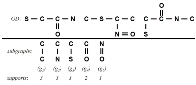
Fig. 3-3 shows a sample graph data set, and some subgraphs with their supports.

In these subgraphs, g1, g2, g3, and g4 are frequent if the minimum support is 2.

Chapter 4

The Graph Mining Algorithm

The discovery of frequent subgraphs usually consists of two steps. In the first

step, we generate frequent subgraph candidates. The frequency of each candidate is

checked in the second step. Therefore, the core of any frequent subgraph mining

algorithm are two computationally challenging problem: (1) subgraph isomorphism:

determine whether a given graph occurs in another graph; and (2) efficient

enumeration of all frequent subgraphs. gSpan introduces two techniques to solve these

problems: The DFS lexicographic ordering and the right-most extension. In this

chapter, we will introduce the general frequent subgraph mining process, and then

describe the procedure of gSpan and those techniques of gSapn. Finally, we will

formulate our proposed graph mining algorithm.

The general framework of a naïve frequent graph mining algorithm is outlined in

Fig. 4-1. We refer to this algorithm as NaïveGraph. In the mining process, a graph g can be extended by adding a new edge e. Let the new graph denoted by g ◊e. Edge e may or may not introduce a new vertex to g. For each discovered graph g, it performs

the extension recursively until all the frequent graphs with g embedded are discovered.

is less than min_sup, it is unnecessary to extend it any more.

Fig. 4-1: A naïve graph mining algorithm. [29]

NaïveGraph is simple, but not efficient. The key issue is the inefficiency of

extending g to g ◊e. The same graph can be extended in different ways. For instance, an n-edge graph may have n different ways to be formed from n different (n-1)-edge

graphs if we do not consider isomorphism. As a result, there may be n-1 duplicate

graphs. Fig. 4-2 shows a graph g and four different ways to generate it. Line 1 in

Algorithm 1 gets rid of duplicate graphs. The number of duplicate graphs may be huge.

It raises some severe problems. First, the generation and support computation of

duplicate graphs waste time. Second, it is nontrivial to tell whether a graph is a

see, these three problems affect the efficiency of the algorithm. gSpan overcomes these

problems by using two techniques: (1) the DFS lexicographic ordering; and (2) the

right-most extension. It has the following salient properties: (1) it reduces the

generation of duplicate graphs; (2) it does not need to search previous discovered

frequent graphs in order to detect duplicates; and (3) it never extends any duplicate

graph but still guarantees the completeness.

Fig. 4-2: Four different ways to generate g

In the following two sections, we focus on the background knowledge of the DFS

code tree. It includes the two major techniques used in gSpan.

4.1 Lexicographic Ordering

This section introduces several techniques developed to represent and extend

a lexicographic ordering among these codes, and mining DFS codes based on this

lexicographic order.

4.1.1 DFS Subscripting

When performing a depth-first search in a graph, a corresponding DFS tree can

be constructed. Fig. 4-3 shows a graph and three different DFS trees of it. The graph

has four vertices with labels x, x, y, z and four edges with labels a, a, b, b. The

subgraphs with darkened edges in Fig. 4-3(b)-(d) show the DFS trees. For a given

graph, there are many ways to construct different DFS trees by selecting different

starting points and different growing edges. When building a DFS tree for a graph G,

the depth-first discovery of the vertices forms a linear order. If there are n vertices in

G, each vertex is assigned a subscript from 0 to n-1 according to the discovery order.

i.e. v0, v1, v2,..., vn-1. v0 is called the root and vn-1 is called the right-most vertex. The

straight path from the root to the right-most vertex is named the right-most path. In

Fig. 4-3(b)-(d), three different subscriptings are generated for the graph in Fig. 4-3(a).

The right-most path is (v0, v1, v3) in Fig 4-3(b) and (c), and (v0, v1, v2, v3) in Fig. 4-3(d).

Incidentally, the darkened edges are forward edges while the undarkened ones are

forward edge; otherwise, a backward edge. The forward edges of vi means the forward

edges started from vi. The backward edges of vi means the backward edges started

from vi.

Fig. 4-3: DFS subscripting. [29]

4.1.2 DFS Code

Since there may be different DFS subscriptings for the same graph, gSpan wants

to select one from them as base subscripting. For this purpose, gSpan maps each

subscripted graph into an edge sequence. Afterwards, it builds an order among these

sequences and selects the subscripting that generates the minimum sequence as its

base subscripting. There are two kinds of orders in this process: (1) edge order, which

introduced.

The DFS tree has defined the discovery order of forward edges. For the graph

shown in Fig. 4-3(b), the forward edges are discovered in the order (0, 1), (1, 2),

(1, 3). Now consider the backward edges, for a given vertex v, all of its backward

edges should appear just before its forward edges. And its backward edges should

appear just after the forward edge where v is the second vertex. For vertex v2 in

Fig.4-3(b), its backward edge (2, 0) should appear just after (1, 2). Among the

backward edges from the same vertex, gSpan enforces an order: Given vi and its two

backward edges, (i, j1), and (i, j2), if j1 < j2, then edge (i, j1) will appear before edge

(i, j2). The ordering of the edges in a graph is now completed. Based on this order, a

graph can be translated into a sequence. A complete sequence for Fig. 4-3(b) is (0, 1),

(1, 2), (2, 0), (1, 3).

gSpan represents an edge by a 5-tuple, ( i, j, l(i), l(i, j), l(j)), where l(i) and l(j)

are the labels of vi and vj respectively and l(i, j) is the label of the edge (vi, vj). For

example, (v0, v1) in Fig. 4-3(b) is represented by (0, 1, X, a, X). For two edges e1 = ( i1,

j1, l(i1), l(i1,j1), l(j1)), and e2 = ( i2, j2, l(i2), l(i2,j2), l(j2)), gSpan defines a linear

order, <T, in R5. e1 <T e2 holds if one of the following statements is true:

(1) e1 and e2 are forward edges, and j1 < j2 or ( (j1 = j2)∧ (i1 > i2) ).

(2) e1 and e2 are backward edges, and i1 < i2 or ( (i1 = i2) ∧ ( j1 < j2) ).

(3) e1 is backward edge and e2 is forward edge, and i1 < j2.

(5) i1 = i2, and j1 = j2 , and li1 < li2 or

li1 = li2 and l(i1,j1) < l(i2,j2) or

l(i1,j1) = l(i1,j1) and lj1 < lj2.

Note that in (1), when j1 = j2, it is i1 > i2.In (5), the two edges have the same

discovery order, so the labels are considered. Fig. 4-4 shows a graph g, and four ways

to extend g. These extensions add edge (2, 0), (2, 3), (1, 3), and (0, 3) to g respectively.

Therefore the order between these edges will be (2, 0) <T (2, 3) <T (1, 3)<T (0, 3).

Fig. 4-4: An example of edge order.

Definition 5 (The DFS code) Given a DFS tree T for a graph G, an edge sequence

(e0, e1, e2,…, e|E|) can be constructed based on <T, such that ei <T ei+1, where i =

0,…,|E|-1. (e0, e1, e2,…, e|E|) is called a DFS code, denoted as code(G,T).

Table 4-1 shows three different DFS codes γ0, γ1, and γ2, which are generated by

DFS trees generate different DFS codes. It is a one-to-one mapping between a

subscripted graph and a DFS code. Thus, we can treat a subscripted graph and its DFS

code as the same. All the notations on subscripted graphs can also be applied to DFS codes. For instance, for a given DFS code α, we can use α ◊ e to represent a possible extension of α. The graph represented by a DFS code α is written as gα.

Table 4-1: DFS codes for the graphs in Fig. 4-3(b)-(d). [29]

4.1.3 DFS Lexicographic Order

gSpan wants to build an order among the DFS codes generated for a graph so

that a minimum DFS code can be defined for this graph. The edge order can be

extended to a sequence order, which is a linear order on DFS codes. The formal

Definition 6 (DFS Lexicographic Order) Given a graph dataset GD, suppose Z =

{code(G, T) | G∈GD, T is a DFS subscripting of G }, i.e., Z is a set containing all DFS codes of all graphs. DFS Lexicographic Order is a linear order defined as follows.

If α = code(Gα, Tα) = (a0, a1,…, am) and β = code(Gβ, Tβ) = (b0, b1,…, bn), α, β ∈ Z,

then α < β if and only if either of the following is true. (1) ∃t, 0 ≤ t ≤ min{m, n},∀k < t, ak = bk, and at <T bt.

(2) ∀k, 0 ≤ k ≤ m , ak =bk, and m ≤ n.

Definition 7 (Minimum DFS Code) Given a graph G, C(G) = {code(G,T) | ∀T, T is

a DFS tree for G}, based on DFS lexicographic order, the minimum one, min(C(G)), is called Minimum DFS Code of G.

According to DFS lexicographic order, we can compare the three DFS codes

listed in Table 4-1. Code γ0 is less than code γ1, which is less than code γ2. Moreover,

γ0 is the minimum DFS code of the graph in Fig. 4-3(a). Minimum DFS code can be

considered as canonical label.

Definition 8 (DFS Code Tree) In a DFS code tree, each vertex represents a DFS

code, the relation between siblings is consistent with the DFS lexicographic order. That is, the pre-order search of DFs code tree follows the DFS lexicographic order.

DFS code and vertex in the DFS code tree are equivalent in the sense that one

can be derived from the other. Any valid DFS code has a unique corresponding vertex

in the DFS code tree, and any vertex in the DFS code tree contains a valid DFS code.

4.2 Right-Most Extension

In Algorithm 1, NaïveGraph requires extending g in any possible position,

which will result in a huge number of duplicate graphs. gSpan adopts a more clever

way to extend graphs. The extension is restricted as follows: Given g and a DFS tree

T in g, e can be extended from the right-most vertex connecting to any other vertices

on the right-most path (backward extension); or e can be extended from vertices on

the right-most path and introduce a new vertex (forward extension). The extension

under these restrictions is named right-most extension, and it is denoted by g ◊r e,

where r indicates that the extension is a right-most extension. For instance, Fig. 4-5

shows all the potential right-most extensions of the graph of Fig.4-3(b). The darkened

edges show the right-most path. The dotted edges are the new edges extended and the

dotted vertices are the new vertices added. For simplicity, we omit labels here. The

backward extension candidates can be (v3, v0). The forward extension candidates can

Fig. 4-5: The graphs extended from the graph in Fig.4-3(b).

Since a graph may have different DFS subscriptings, the right-most extension

may generate many duplicate graphs if we need to extend all the subscriptings. The

following theorem shows that we only need to conduct the right-most extension on the

base subscripting.

Theorem 1 (Completeness) Performing right-most extension in NaïveGraph

guarantees the completeness of the mining result. Furthermore, performing only the right-most extension on the minimum DFS codes guarantees the completeness of the mining result.

When performing the right-most extension in NaïveGraph, it is possible that a DFS code α is minimum, but α ◊r e is not. For instance, Fig. 4-6 shows a graph g with

a minimum DFS code, but one extension of g is not minimum. In this case, we do not

Fig. 4-6 An example of non-minimum DFS code

4.3 gSpan

In this section, we formulate the algorithm of gSpan based on the DFS

lexicographic order and the right-most extension. gSpan uses a sparse adjacency list

representation to store graphs. The procedure of gSpan can be illustrated with a DFS

code tree. The mining process is equivalent to a pre-order traversal of the DFS code

tree, which enumerates all frequent subgraphs of a graph database. The pre-order

search of DFS code tree follows the DFS lexicographic order. Fig. 4-7 shows an

example of the search space of gSapn, where each vertex of the tree represents a DFS

Fig. 4-7: A DFS code tree.

Fig. 4-8: The pseudo code of gSpan. [28]

The difference between gSpan and NaïveGraph is the right-most extension and

existence judgement in Algorithm 1 Line 1 by checking whether s is minimum.

Actually, the checking is more efficient to calculate. It prunes all DFS codes which

are not minimum. It significantly reduces unnecessary computation on duplicate

subgraphs and their descendants. Fig. 4-9 outlines an algorithm for checking whether

s is minimum. Fig. 4-10 shows the search space of gSpan, If we find two DFS codes s

and s’ representing the same graph and s < s’, by Theorem 1, we can completely stop

searching any descendant of s’.

Fig. 4-10: The search space of gSpan. [28]

4.4 The Proposed Enumeration Method

Given a graph g with n vertices, v0, v1,…, vn, assume the length of its right-most

path is k. The right-most path of g can be represented by a sequence of (k+1) vertices

which starts from v0 and ends at vn. For the sake of simplicity, we denote the vertices

of the right-most path as r0, r1, …, rk. When performing right-most extension on g, we

denote the backward extensions as g ◊b0 e, g ◊b1 e, …, g ◊b(k-2) e , where g ◊bi e means

a backward extension of g which adds a backward edge (rk, ri). Similarly, we denote

the forward extension as g ◊f1 e, g ◊f2 e, …, g ◊fk e,where g ◊fi e means a forward

graph g and the corresponding extensions. The right-most path of g is (r0 , r1, r2, r3).

Fig. 4-11: A right-most extension.

There are two duplicate graphs in Fig. 4-11, g ◊f1 e and g ◊f0 e . In this case, the

two extensions are redundant. We want to shrink the search space by removing some

redundant extensions from the right-most extension. We propose an additional

restriction to the right-most extension. In the following section we will introduce this

modified extension.

For a given graph g with a right-most path (r0, r1, …, rk), in the forward

extensions, the operations ◊f0, ◊f1, …, ◊fk/2 are redundant, that is, graphs generated

by these operations are duplicate. For instance, in Fig. 4-11, f0 and f1 are not necessary.

The backward extensions remain unchanged. In order to prove the completeness of

Conjecture (Symmetry of Graph) Given a graph g, along its right-most path (r0,

r1, …, rk), we can find a graph g’, which is symmetric to g with respect to the center of

its right-most path.

According to this conjecture, for every graph g, there exists a graph g’, such that

g ◊f0 e = g’ ◊fk e. Thus, we can discard the operation f0 and still guarantee the

completeness of the mining result. For the same reason, we can remove all the

operation fi, i=0,1,…,k/2 from the right-most extension.

By replacing the right-most extension of gSpan with this modified right-most

Chapter 5

Experimental Results

Since the complexity of graph mining is higher when mines unlabeled graph

datasets, we conduct a performance study on unlabeled datasets. On both synthetic

and real world datasets, the experiments are performed. We use a synthetic data

generator provided by Kuramochi and Karypis[16]. The real data set we tested is a

chemical compound dataset with the labels removed. All experiments are done on a

3.0GHz Intel Pentium D PC with 2GB memory, running Windows XP system. Our

performance tests show that the number of candidates generated by our algorithm is

about 10% less than that generated by gSpan.

We use the data generator provided by Kuramochi. The parameter description of

the data generator is shown in Table 5-1. The synthetic datasets are generated using a

similar procedure described in [1]. Kuramochi et al. applied a simplified procedure in

their graph data synthesis. The details about how to generate the datasets were

described in [16]. The generator generates |D| graphs. The size of each graph is a

Poisson random variable whose mean is equal to |T|. In our experiments, some

parameters of the data generator are fixed value: |T|=10, |I|=6, and |S|=200. Since the

Table 5-1: Synthetic dataset parameters

We test the performance of our algorithm on a synthetic dataset with |D| = 10k.

Fig. 5-1 shows the number of candidates generated by our proposed algorithm and

Fig. 5-1: Number of candidates (synthetic dataset).

The chemical compound dataset is the same one used in [16,28], This was

originally provided for the Predictive Toxicology Evaluation Challenge [36], which

contains information on 340 chemical compounds. We set all the labels to a same

label to transform this dataset to a unlabeled dataset. There are 340 graphs in total.

The average graph size is 27.4 in terms of the number of edges and 27.0 in terms of

the number of vertices. There are 26 graphs that have more than 50 edges and vertices.

The largest graph contains 214 edges and 214 vertices. We test the performance on

this chemical compound dataset. Fig. 5-2 illustrates the number of candidates

Fig. 5-2: Number of candidates (chemical compound dataset).

The experimental results show that the number of candidates generated by our

proposed algorithm is about 5%~10% less than that generated by gSpan. In our

experiments, the mining result is correct, in other words, the completeness of our

proposed enumeration method is fulfilled. Unfortunately, we have not completed a

formal proof for the completeness. There is still a possibility that our proposed

algorithm works only on some special cases. We require further research and

Chapter 6

Conclusion and Future Works

In this thesis, we analyzed the state-of-the-art graph mining algorithm gSpan and

addressed the possible inefficiencies in it. We found that when gSpan deals with large

and complex graphs (denser graphs with fewer labels available), especially when

deals with unlabeled graphs, the performance of gSpan degrades. Based on gSpan, we

proposed a new graph enumeration method, which reduces the candidate generation.

There are still some research issues of our proposed algorithm. First, we have to

prove the completeness of our proposed algorithm. Second, there might be a better

algorithm to calculate the minimum code when the graph is unlabeled. Third, in order

to extend our algorithm to mine labeled graphs, we might require a new lexicographic

order. Therefore, to develop a new lexicographic order for our proposed algorithm is a

Bibliography

[1] R. Agrawal and R. Srikant. “Fast algorithms for mining association rules”, in Proc. 1994 Int. Conf. Very Large Data Bases (VLDB’94), pp.487-499, Santiago, Chile, September 1994.

[2] R. Agrawal and R. Srikant. “Mining sequential patterns”, in Proc. 1995 Int. Conf. Data Engineering (ICDE’95), pp.3-14, Taipei, Taiwan, March 1995.

[3] T. Asai, K. Abe, S. Kawasoe, H. Arimura, H. Satamoto, and S. Arikawa. “Efficient substructure discovery from largesemi-structured data”, in Proc. 2002 SIAM Int. Conf. Data Mining, Arlington, VA, April 2002.

[4] R. Attias and J. E. Dubois. “Substructure systems: concepts and classifications”, Journal of Chemical Information and Computer Sciences, Volume 30, pp.2-7 1990.

[5] D. M. Bayada, R. W. Simpson, and A. P. Johnson. “An algorithm for the multiple common subgraph problem”, Journal of Chemical Information and Computer Science, Volume 32, pp.680-685, 1992.

[6] R. J. Bayardo. “Efficiently mining long patterns from databases”, in Proc. 1998 ACM-SIGMOD Int. Conf. Management of Data (SIGMOD’98), pp.85-93, Seattle, WA, June 1998.

[7] D. Burdick, M. Calimlim, and J. Gehrke. MAFIA: “A maximal frequent itemset algorithm for transactional databases”, in Proc. 2001 Int. Conf. Data Engineering (ICDE’01), pp.443-452, Heidelberg, Germany, April 2001.

[8] L. P. Cordella, P. Foggia, C. Sansone, and M. Vento. “Graph matching: A fast algorithm and its evaluation”, in Proceedings of the 14th Int. Conf. on Pattern Recognition(ICPR-16), pp.1582-1584, August 1998.

[9] T. H. Cormen, C. E. Leiserson, R. L. Rivest, and C. Stein. Introduction to Algorithms, MIT Press, 2001 Second Edition.

[10] L. Dehaspe, H. Toivonen, and R. King. “Finding frequent substructures in chemical compounds”, in Proc. 1998 Int. Conf. Knowledge Discovery and Data

Mining (KDD’98), pp.30-36, New York, August. 1998.

[11] S. Fortin. “The graph isomorphism problem”, Technical Report TR96-20, Department of Computing Science, University of Alberta, July 1996.

[12] B. Liu, G. Cong, L. Yi, and K. Wang. “Discovering frequent substructures from hierarchical semi-structured data”, in Proc. 2002 SIAM Int. Conf. Data Mining, Arlington, VA, April 2002.

[13] J. Han, J. Pei, and Y. Yin. “Mining frequent patterns without candidate generation”, in Proc. 2000 ACM-SIGMOD Int. Conf. Management of Data (SIGMOD’00), pp.1-12, Dallas, TX, May 2000.

[14] L. B. Holder, D. J. Cook, and S. Djoko. “Substructure discovery in the subdue system”, in Proc. AAAI’94 Workshop Knowledge Discovery in Database (KDD’94), pp.169-180, Seattle, WA, July 1994.

[15] A. Inokuchi, T. Washio, and H. Motoda. “An apriori-based algorithm for mining frequent substructures from graph data”, in Proc. of the 4th European Conf. on Principles and Practice of Knowledge Discovery in Databases ( PKDD’00), pp.13-23, Lyon, France, September 2000.

[16] M. Kuramochi and G. Karypis. “Frequent subgraph discovery”, in Proc. 2001 Int. Conf. Data Mining (ICDM’01), pp.313-320, San Jose, CA, November 2001.

[17] H. Mannila, H. Toivonen, and A. I. Verkamo. “Discovery of frequent episodes in event sequences”, Data Mining and Knowledge Discovery, pp.259-289, 1997.

[18] B. D. McKay. “Practical graph isomorphism”, Congressus Numerantium, pp.45-97, 1981

[19] J. Pei, J. Han, B. Mortazavi-Asl, H. Pinto, Q. Chen, U. Dayal, and M.-C. Hsu. “PrefixSapn: Mining sequential patterns efficiently by prefix-projected pattern growth”, in Proc. 2001 Int. Conf. Data Engineering (ICDE’01), pp.215-224, Heidelberg, Germany, April 2001.

[20] K. Shearer, H. Bunke, and S. Venkatesh. “Video indexing and similarity retrieval by largest common subgraph detection using decision trees”, Pattern

Recognition, pp.1075-1091, 2001.

[21] P. Shenoy, J. R. Haritsa, S. Sudarshan, G. Bhalotia, M. Bawa, and D. Shah. “Turbo-charging vertical mining of large databases”, in Proc. 2000 ACM-SIGMOD Int. Conf. Management of Data (SIGMOD’00), pp.22-33, Dallas, TX, May 2000.

[22] S. Su, D. J. Cook, and L. B. Holder. “Knowledge discovery in molecular biology: Identifying structural regularities in proteins”, Intelligent Data Analysis, pp.413-436, 1999.

[23] Y. Takahashi, Y. Satoh, and S. Sasaki. “Recognition of largest common fragment among a variety of chemical structures”, Analytical Science, pp.23-28, 1987.

[24] J. R. Ullmann. “An algorithm for subgraph isomorphism”, Journal of the ACM, pp.31-42, 1976.

[25] E. K. Wong. “Model matching in robot vision by subgraph isomorphism”, Pattern Recognition, pp.287-304, 1992.

[26] M. J. Zaki. “Efficiently mining frequent trees in a forest”, in Proc. of the 2002 Conf. on Knowledge Discovery and Data Mining (SIGKDD’02), 2002.

[27] M. J. Zaki and C. J. Hsiao. “CHARM: An efficient algorithm for closed itemset mining”, in Proc. 2002 SIAM Int. Conf. Data Mining, pp.457-473, Arlington, VA, April 2002.

[28] X. Yan and J. Han. “gSpan: Graph-based substructure pattern mining”, in Proc. 2002 Int. Conf. Data Mining (ICDM’02), pp.721-724, 2002 .

[29] X. Yan and J. Han. “Closegraph: Mining closed frequent graph patterns”, in Proc. of the 2003 Conf. on Knowledge Discovery and Data Mining (SIGKDD’03), 2003.

[30] S. Nijssen, J. N. Kok. “A quickstart in frequent structure mining can make a difference”, in Proc. of the 2004 Conf. on Knowledge Discovery in Databases

[31] M. R. Garey and D. S. Johnson. “Computers and intractability: A guide to the theory of NP-completeness”, New York: W. H. Freeman, 1979.

[32] L. Dehaspe and H. Toivonen . “Discovery of frequent datalog patterns”, Data Mining and Knowledge Discovery, pp.7-36, 1999.

[33] C. Borgelt and M. R. Berhold. “Mining molecular fragments: Finding relevant substructures of molecules”, in Proc. 2002 Int. Conf. Data Mining (ICDM’02), pp.51-58, 2002.

[34] J. Huan, W. Wang, J. Prins. “Efficient mining of frequent subgraphs in the presence of isomorphism”, in Proc. 2003 Int. Conf. Data Mining (ICDM’03), pp.549-552, 2003.

[35] A. Inokuchi, T. Washio, and H. Motoda. “Complete mining of frequent patterns from graphs: Mining graph data”, Machine Learning, Volume 50, pp.321-354, 2003.

[36] A. Srinivasan, R. D. King, S. H. Muggleton, and M. Sternberg. “The predictive toxicology evaluation challenge”, in Proc. of the 15th Int. Joint Conf. on Artificial Intelligence (IJCAI), pp. 1–6. Morgan-Kaufmann, 1997.

[37] J. Han, H. Cheng, D. Xin, and X. Yan. “Frequent pattern mining: current status and future directions.” Data Mining and Knowledge Discovery, pp.55-86, 2007.

[38] M. Worlein, T. Meinl, I. Fischer, and M. Philippsen. “A Quantitative Comparison of the Subgraph Miners MoFa, gSpan, FFSM, and Gaston”, in proc. of the 9th European Conf. on Principles and Practice of Knowledge Discovery in Databases (PKDD’05), pp.392-403, 2005.