最大利潤下規格上限與EWMA管制圖之設計 - 政大學術集成
97
0
0
全文
(2) 謝辭 研究生生活即將結束,這兩年我過得很充實,學到了許多寶貴的知識以及經 驗,讓我成長不少,這一切必須感謝很多人這些日子以來的幫助與支持。 首先最要感謝的是我的指導老師 楊素芬教授。謝謝楊老師這兩年對我的辛 苦栽培,讓我學習到許多統計品管上的知識,更重要的是了解做人處世的道理。 老師嚴格的指導,讓我能更加積極地去面對任何事情。也謝謝老師對我碩士論文 的協助,讓英文不優的我,能順利完成此篇論文。 接著要感謝我的口試委員,曾勝滄教授與 葉小蓁教授;感謝兩位教授在百 忙之中抽出時間閱讀論文以及前來政大擔任口試委員。更要謝謝兩位教授對論文 提出寶貴的建議與想法,讓我能加以改進,使本篇論文更加完善。也要謝謝兩位 教授在口試後所給予的勉勵與祝福。 碩士兩年期間,要感謝我的同學們為我打氣以及給予我的幫助。有大家的陪 伴,讓我能度過許多艱辛的日子。有大家一起玩樂,也讓我更有動力去完成許多 事情。特別要感謝瑋倫和依潔,謝謝你們在研究上給予我的協助,有幸能與你們 討論,讓我解決許多困難的問題。 最後一定要感謝的是我的家人,謝謝你們給我的鼓勵與支持,更要謝謝你們 讓我能無後顧之憂的專心處理課業上的事情。你們永遠是我最大的支柱,往後的. 立. 政 治 大. ‧ 國. 學. ‧. 日子我也將更加努力,並且希望能對這個家有所貢獻。 本研究承蒙行政院國家科學委員會,計畫編號NSC100-2118-M-004-003-MY2 補助,謹此致謝。 此項成果使用國家高速網路與計算中心之計算資源,特此感謝。. n. er. io. sit. y. Nat. al. Ch. engchi. i n U. v. 蔡佳宏 謹致 中華民國一百零一年六月 I.
(3) ABSTRACT The determination of economic control charts and the determination of specification limits with minimum cost are two different research topics. In this study, we first combine the design of economic control charts and the determination of specification limits to maximize the expected profit per unit time for the smaller the better quality variable following the gamma distribution. Because of the asymmetric distribution, we design the EWMA control chart with asymmetric control limits. We simultaneously determine the economic EWMA control chart and upper specification limit with maximum expected profit per unit time. Then, extend the approach to determine the economic variable sampling interval EWMA control chart and upper specification limit with maximum expected profit per unit time. In all our numerical examples of the two profit models, the optimum expected profit per unit time under inspection is higher than that of no inspection. The detection ability of the EWMA chart with an appropriate weight is always better than the X-bar probability chart. The detection ability of the VSI EWMA chart is also superior to that of the fixed sampling interval EWMA chart. Sensitivity analyses are provided to determine the significant parameters for the optimal design parameters and the. 立. 政 治 大. ‧ 國. 學. ‧. optimal expected profit per unit time.. n. al. er. io. sit. y. Nat. Keywords: Economic design; Specification; EWMA control chart; VSI control chart; Markov chain; Gamma distribution; Optimization technique. Ch. engchi. II. i n U. v.
(4) TABLE OF CONTENTS CHAPTER 1.. INTRODUCTION ......................................................................... 1. 1.1 Research Motivation .......................................................................................... 1 1.2 Literature Review ............................................................................................... 1 1.3 Research Method................................................................................................ 3 CHAPTER 2.. THE SMALLER THE BETTER QUALITY VARIABLE WITH GAMMA DISTRIBUTION ............................................. 4. 2.1 In-control Sampling Distribution of X-bar under Gamma Distribution ............ 4 2.2 Out-of-control Sampling Distribution of X-bar under Gamma Distribution ..... 4. 政 治 大 Distribution ........................................................................................................ 5 立. 2.3 Construction of the EWMAX-bar Control Chart Based on X-bar Sampling. ‧ 國. 學. 2.4 Calculation of Average Run Length for the EWMAX-bar Chart.......................... 6 2.5 Determining Control Limit Coefficient on EWMAX-bar Control Chart under. ‧. Different n and λ................................................................................................. 7. y. sit. io. DERIVATION OF THE PROFIT MODEL WITHOUT PRODUCER INSPECTION ...................................................... 19. n. al. er. CHAPTER 3.. Nat. 2.6 Determining the Best λ in the EWMAX-bar Chart under Different δ1, δ2 and n 11. i n U. v. 3.1 Derivation of Expected Cycle Time ................................................................. 19. Ch. engchi. 3.2 Derivation of the Expected Cycle Profit .......................................................... 20 3.3 Determining Optimum Design Parameters of the Economic EWMAX-bar Control Chart.................................................................................................... 21 3.4 An Example...................................................................................................... 22 3.5 Sensitivity Analysis and Comparing the Results with λ=1 .............................. 23 CHAPTER 4.. DERIVATION OF THE PROFIT MODEL WITH PRODUCER INSPECTION ...................................................... 28. 4.1 Derivation of the Expected Cycle Time ........................................................... 28 4.2 Derivation of the Expected Cycle Profit .......................................................... 28. III.
(5) 4.3 Determining the Optimum Producer Inspection and Design Parameter of the Economic EWMAX-bar Control Chart............................................................... 29 4.4 Example and Optimum Results Comparison for with and without Producer Inspection ......................................................................................................... 30 4.5 Sensitivity Analysis and Comparing the Results of EWMAX-bar Chart with λ=1 .................................................................................................................... 32 CHAPTER 5.. DETERMINING THE BEST λ OF THE ECONOMIC EWMAX-bar CONTROL CHART UNDER DIFFERENT SHIFT SCALES IN THE MEAN AND VARIANCE .............. 37. 政 治 大 the Design Parameters of the Economic EWMA Control Chart ............... 37 立. 5.1 Data Description and Determining the Optimum Producer Inspection and X-bar. DETERMINING. THE. 學. CHAPTER 6.. ‧ 國. 5.2 Performance Comparison of Six Numerical Examples ................................... 63 OPTIMUM. PRODUCER. ‧. INSPECTION AND THE ECONOMIC VSI EWMAX-bar CONTROL CHART ................................................................... 65. sit. y. Nat. 6.1 VSI EWMAX-bar Control Chart and ATS Calculation....................................... 65. io. er. 6.2 Derivation of the Profit Model without Producer Inspection........................... 67 6.3 Derivation of the Profit Model with Producer Inspection ................................ 67. al. n. v i n Optimum CParameters of the U h e n g c h i Economic. 6.4 Determining. VSI EWMAX-bar. Control Chart with and without producer tolerance ......................................... 68 6.5 Two Numerical Examples and the Results Comparison with the FSI EWMAX-bar Control Chart ................................................................................ 69 6.6 Sensitivity Analysis and the Optimum Results Comparison between the FSI EWMAX-bar Chart and VSI EWMAX-bar Chart ................................................. 80 CHAPTER 7. SUMMARY ................................................................................. 84 REFERENCES …………………………………………………………………...86. IV.
(6) LIST OF TABLES Table 2-1. The solved L1 and L2 under various combinations of λ and n for aI=1.5, bI=2, ARL0=370 and g=301.................................................................................... 8 Table 2-2. The solved L1 and L2 under various combinations of λ and n for aI =24.349, bI=0.205, ARL0=370 and g=301 ............................................................. 9 Table 2-3. The solved L1 and L2 under various combinations of λ and n for aI =1, bI=0.202, ARL0=370 and g=301........................................................................... 10 Table 2-4. The Value of ARL1 under Various n and λ at aI =1.5, bI =2, δ1=0.1, δ2=0.05, g=301 and ARL0=370 ............................................................................ 11 Table 2-5. The Value of ARL1 under Various n and λ at aI =24.349, bI =0.205,. 政 治 大 Table 2-6. Combination of λ, n, L and L with Minimum ARL ................................. 12 立 Table 2-7. The Value of ARL under Various n and λ at a =24.349, b =0.205, δ1=0.919, δ2=0.06, g=301 and ARL0=370 ............................................................ 12 1. 2. 1. 1. I. I. ‧ 國. 學. δ1=16.983, δ2=-0.045, g=301 and ARL0=370....................................................... 13 Table 2-8. Combination of λ, n, L1 and L2 with Minimum ARL1 ................................. 13. ‧. Table 2-9. The Value of ARL1 under Various n and λ at aI =24.349, bI =0.205,. y. Nat. δ1=-8.741, δ2=0.123, g=301 and ARL0=370......................................................... 14. sit. Table 2-10. Combination of λ, n, L1 and L2 with Minimum ARL1 ............................... 14. er. io. Table 2-11. The Value of ARL1 under Various n and λ at aI =24.349, bI =0.205,. al. v i n C L with Minimum Table 2-12. Combination of λ, n, Lhand e n g c h i U ARL ............................... 15 n. δ1=9.452, δ2=-0.097, g=301 and ARL0=370......................................................... 15 1. 2. 1. Table 2-13. The Value of ARL1 under Various n and λ at aI =1, bI =0.202, δ1=0,. δ2=0.077, g=301 and ARL0=370 .......................................................................... 16 Table 2-14. Combination of λ, n, L1 and L2 with Minimum ARL1 ............................... 16 Table 2-15. The Value of ARL1 under Various n and λ at aI =1, bI =0.202, δ1=0, δ2=0.442, g=301 and ARL0=370 .......................................................................... 17 Table 2-16. Combination of λ, n, L1 and L2 with Minimum ARL1 ............................... 17 Table 2-17. The Best λ in Tables 2-4, 2-5,…, 2-16. .................................................... 18 Table 3-1. Optimum Results of Profit Model under Three Different λ ....................... 22 Table 3-2. Level of Parameters .................................................................................... 23 Table 3-3. Parameters for Each Experiment ................................................................ 23 V.
(7) Table 3-4. Optimum Results in Each Experiment ....................................................... 24 Table 4-1. Optimum Results of Profit Model under Three Different λ ....................... 30 Table 4-2. Merging Tables 3-1 and 4-1 ....................................................................... 31 Table 4-3. Optimum Result in Each Experiment ......................................................... 32 Table 5-1. In-control Data with Gamma (a=25, b=0.2)............................................... 37 Table 5-2. Out-of-control Data with Gamma (a=26, b=0.25) ..................................... 38 Table 5-3. The Optimum Results Comparison of Profit Model with Different λ ........ 39 Table 5-4. Out-of-control Data with Gamma (a=28, b=0.21) ..................................... 42 Table 5-5. The Optimum Results Comparison of Profit Model with Different λ ........ 43 Table 5-6. Out-of-control Data with Gamma (a=42.45, b=0.154) .............................. 46. 政 治 大. Table 5-7. The Optimum Results Comparison of Profit Model with Different λ ........ 47. 立. Table 5-8. Out-of-control Data with Gamma (a=15.385, b=0.325) ............................ 50. ‧ 國. 學. Table 5-9. The Optimum Results Comparison of Profit Model with Different λ ........ 51 Table 5-10. Out-of-control Data with Gamma (a=15.385, b=0.325) .......................... 54. ‧. Table 5-11. The Optimum Results Comparison of Profit Model with Different λ ...... 55 Table 5-12. In-control Service Time Data. .................................................................. 58. y. Nat. sit. Table 5-13. Out-of -control Service Time Data. .......................................................... 59. n. al. er. io. Table 5-14. The Optimum Results Comparison of Profit Model with Different λ ...... 60. i n U. v. Table 5-15. Comparison of Six Numerical Examples ................................................. 63. Ch. engchi. Table 6-1. Comparison of the optimum results of VSI and FSI EWMAX-bar control charts .................................................................................................................... 70 Table 6-2. Comparison of the optimum results of the VSI and FSI EWMA X-bar charts at λ=0.4 ...................................................................................................... 71 Table 6-3. Region and Sampling Time of Each In-control Statistic (λ=0.4) ............... 74 Table 6-4. Region and Sampling Time of Each Out-of-control Statistic (λ=0.4) ........ 75 Table 6-5. Comparison of the optimum results of the VSI and FSI EWMA X-bar charts at λ=0.1 ...................................................................................................... 76 Table 6-6. Region and Sampling Time of Each In-control Statistic (λ=0.1) ............... 78 Table 6-7. Region and Sampling Time of Each Out-of-control Statistic (λ=0.1) ........ 79 Table 6-8. Optimum Results in Each Experiment ....................................................... 80 VI.
(8) LIST OF FIGURES. Figure 2-1. The p.d.f Comparison of Different Gamma Distributions .......................... 4 Figure 2-2. States between the Control Limits of EWMAX-bar Chart ............................ 6 Figure 2-3. The Value of L1 under Various n at ARL0=370, aI =1.5, bI =2 and g=301 .. 8 Figure 2-4. The Value of L2 under Various n at ARL0=370, aI =1.5, bI =2 and g=301 .. 8 Figure 2-5. The Value of L1 under Various n at ARL0=370, aI =24.349, bI =0.205 and g=301............................................................................................................... 9 Figure 2-6. The Value of L2 under Various n at ARL0=370, aI =24.349, bI =0.205 and g=301............................................................................................................... 9. 政 治 大. Figure 2-7. The Value of L1 under Various n at ARL0=370, aI =1, bI =0.202 and g=301 ................................................................................................................... 10. 立. Figure 2-8. The Value of L2 under Various n at ARL0=370, aI =1, bI =0.202 and. ‧ 國. 學. g=301 ................................................................................................................... 10 Figure 3-1. Continuous Process Cycle. ........................................................................ 19. ‧. Figure 3-2. Response Figure of EAP * ....................................................................... 25 Figure 3-3. Response Figure of n * ............................................................................ 25. y. Nat. er. io. sit. Figure 3-4. Response Figure of ARL1 ........................................................................ 26. al. Figure 3-5. Response Figure of UCL * ....................................................................... 26. n. v i n LCL * ....................................................................... Figure 3-6. Response Figure of C 27 hengchi U Figure 3-7. Response Figure of Difference of EAP* ................................................. 27 Figure 4-1. The Gamma Distribution and Taguchi Loss Function with Inspection .... 28 Figure 4-2. Response Figure of * ........................................................................... 33 Figure 4-3. Response Figure of EAP * ....................................................................... 34 Figure 4-4. Response Figure of n * ............................................................................ 34 Figure 4-5. Response Figure of ARL1 .......................................................................... 35 Figure 4-6. Response Figure of UCL * ....................................................................... 35 Figure 4-7. Response Figure of LCL * ....................................................................... 36 Figure 4-8. Response Figure of Difference of EAP* ................................................. 36 Figure 5-1. The Economic EWMAX-bar Chart (λ=1) with In-control Data .................. 40 VII.
(9) Figure 5-2. The Economic EWMAX-bar Chart (λ=1) with Out-of-control Data ........... 40 Figure 5-3. The Economic EWMAX-bar Chart (λ=0.6) with In-control Data ............... 40 Figure 5-4. The Economic EWMAX-bar Chart (λ=0.6) with Out-of-control Data ........ 41 Figure 5-5. The Economic EWMAX-bar Chart (λ=0.05) with In-control Data ............. 41 Figure 5-6. The Economic EWMAX-bar Chart (λ=0.05) with Out-of-control Data ...... 41 Figure 5-7. The Economic EWMAX-bar Chart (λ=1) with In-control Data .................. 44 Figure 5-8. The Economic EWMAX-bar Chart (λ=1) with Out-of-control Data ........... 44 Figure 5-9. The Economic EWMAX-bar Chart (λ=0.5) with In-control Data ............... 44 Figure 5-10. The Economic EWMAX-bar Chart (λ=0.5) with Out-of-control Data ...... 45 Figure 5-11. The Economic EWMAX-bar Chart (λ=0.05) with In-control Data ........... 45. 政 治 大. Figure 5-12. The Economic EWMAX-bar Chart (λ=0.05) with Out-of-control Data .... 45. 立. Figure 5-13. The Economic EWMAX-bar Chart (λ=1) with In-control Data ................ 48. ‧ 國. 學. Figure 5-14. The Economic EWMAX-bar Chart (λ=1) with Out-of-control Data ......... 48 Figure 5-15. The Economic EWMAX-bar Chart (λ=0.6) with In-control Data ............. 48. ‧. Figure 5-16. The Economic EWMAX-bar Chart (λ=0.6) with Out-of-control Data ...... 49 Figure 5-17. The Economic EWMAX-bar Chart (λ=0.05) with In-control Data ........... 49. y. Nat. sit. Figure 5-18. The Economic EWMAX-bar Chart (λ=0.05) with Out-of-control Data .... 49. n. al. er. io. Figure 5-19. The Economic EWMAX-bar Chart (λ=1) with In-control Data ................ 52. i n U. v. Figure 5-20. The Economic EWMAX-bar Chart (λ=1) with Out-of-control Data ......... 52. Ch. engchi. Figure 5-21. The Economic EWMAX-bar Chart (λ=0.3) with In-control Data ............. 52 Figure 5-22. The Economic EWMAX-bar Chart (λ=0.3) with Out-of-control Data ...... 53 Figure 5-23. The Economic EWMAX-bar Chart (λ=0.05) with In-control Data ........... 53 Figure 5-24. The Economic EWMAX-bar Chart (λ=0.05) with Out-of-control Data .... 53 Figure 5-25. The Economic EWMAX-bar Chart (λ=1) with In-control Data ................ 56 Figure 5-26. The Economic EWMAX-bar Chart (λ=1) with Out-of-control Data ......... 56 Figure 5-27. The Economic EWMAX-bar Chart (λ=0.2) with In-control Data ............. 56 Figure 5-28. The Economic EWMAX-bar Chart (λ=0.2) with Out-of-control Data ...... 57 Figure 5-29. The Economic EWMAX-bar Chart (λ=0.05) with In-control Data ........... 57 Figure 5-30. The Economic EWMAX-bar Chart (λ=0.05) with Out-of-control Data .... 57 Figure 5-31. The Economic EWMAX-bar Chart (λ=1) with In-control Data ................ 61 VIII.
(10) Figure 5-32. The Economic EWMAX-bar Chart (λ=1) with Out-of-control Data ......... 61 Figure 5-33. The Economic EWMAX-bar Chart (λ=0.4) with In-control Data ............. 61 Figure 5-34. The Economic EWMAX-bar Chart (λ=0.4) with Out-of-control Data ...... 62 Figure 5-35. The Economic EWMAX-bar Chart (λ=0.1) with In-control Data ............. 62 Figure 5-36. The Economic EWMAX-bar Chart (λ=0.1) with Out-of-control Data ...... 62 Figure 6-1. VSI Control Chart ..................................................................................... 65 Figure 6-2. The Economic FSI EWMAX-bar Chart (λ=0.4) with In-control Data ........ 73 Figure 6-3. The Economic FSI EWMAX-bar Chart (λ=0.4) with Out-of-control Data . 73 Figure 6-4. The Economic VSI EWMAX-bar Chart (λ=0.4) with In-control Data ........ 74 Figure 6-5. The Economic VSI EWMAX-bar Chart (λ=0.4) with Out-of-control Data 75. 政 治 大. Figure 6-6. The Economic FSI EWMAX-bar Chart (λ=0.1) with In-control Data ........ 77. 立. Figure 6-7. The Economic FSI EWMAX-bar Chart (λ=0.1) with Out-of-control Data . 77. ‧ 國. 學. Figure 6-8. The Economic VSI EWMAX-bar Chart (λ=0.1) with In-control Data ........ 78 Figure 6-9. The Economic VSI EWMAX-bar Chart (λ=0.1) with Out-of-control Data 79. ‧. Figure 6-10. Response Figure of * ......................................................................... 81 Figure 6-11. Response Figure of EAP * ..................................................................... 81. y. Nat. sit. Figure 6-12. Response Figure of ATS1 ......................................................................... 82. n. al. er. io. Figure 6-13. Response Figure of UWL * .................................................................... 82. i n U. v. Figure 6-14. Response Figure of LWL * .................................................................... 83. Ch. engchi. Figure 6-15. Response Figure of Difference of EAP* ............................................... 83. IX.
(11) CHAPTER 1. INTRODUCTION. 1.1 Research Motivation Control charts are widely used in statistical process control, and their design parameters must be pre-determined for their use, such as sample size, sampling time, and control limits. Economic design of control charts have been widely used to determine these parameters from economic viewpoint. However, to reduce product quality loss, the 100% inspection with specification limits is always performed. To determine the specification limits, a widely use method is to minimize products cost. In the technology industry, like the product’s insulation property, its loss of heat is the smaller the better. In the service industry, the service time is also the smaller the better. How to determine their specification limits and control chart to monitor the quality variable with maximum profit is an important issue. In this project, we simultaneously determine the specification limits and the control chart parameters with maximize expected profit per unit time. Most articles on economic design of specification and control charts consider normal distribution of quality variable, but in this article, we. 立. 政 治 大. ‧ 國. 學. ‧. consider gamma distribution for the smaller the better quality variable; hence, we determine only an upper specification limit in the gamma distribution. For wide use of different shift scales and because of the asymmetric gamma distribution, we design the asymmetric economic EWMAX-bar control chart and the asymmetric economic VSI EWMAX-bar control chart. Hence, we combine product cost and control chart cost in a profit model and then we maximize this profit per unit time to determine the. n. er. io. sit. y. Nat. al. Ch. i n U. v. optimum upper specification limit and the design parameters of the EWMAX-bar control chart and the VSI EWMAX-bar control chart.. engchi. 1.2 Literature Review Economic design of control charts have been widely used to determine control chart parameters from economic viewpoint. Duncan (1956) first proposed the concept of an economic design for the X-bar control chart. He considered a process that does not shut down when the assignable cause is searched, and developed a process cost model that includes the cost of sampling and finding the assignable cause when it exists or when none exists. He also demonstrated how to determine control chart parameters. Montgomery (1980) presented a review and literature survey in the economic design of control charts. Panagos, Heikes, and Montgomery (1985) described two continuous and discontinuous manufacturing process models, where the 1.
(12) continuous process model is consistent with that developed by Duncan. They showed that the wrong choice of a process model would have a potentially serious economic result. Control charts typically take a fixed number of samples with a fixed sampling time and plot them on the control chart with a fixed control limit. To improve control chart performance, the adaptive control chart has been developed such as variable sampling interval control chart. Reynolds et al. (1988) proposed the VSI X-bar control chart. Bai and Lee (1998) considered the economic design of the VSI X-bar control chart. They preferred to use only two sampling interval lengths with two sub-regions between the two control limits. The EWMA chart is widely used for detecting small process shifts. Roberts (1959) first introduced the exponentially weighted moving average chart. Crowder (1987) and Saccucci and Lucas (1990) discussed the ARL calculation of the EWMA control chart. Montgomery et al. (1995) presented a statistically constrained economic design of the EWMA control chart. They minimized the cost model, subject to statistical constraints on average run length or average time to signal, to determine the. 立. 政 治 大. ‧ 國. 學. ‧. design parameters of the EWMA control chart. Chou et al. (2006) proposed an economic design of VSI EWMA charts. They considered two sampling interval lengths and derived the cost model to determine the parameters of VSI EWMA control charts using the genetic algorithm.. er. io. sit. y. Nat. al. v. n. To reduce product quality loss, the 100% inspection with specification limits is. Ch. i n U. necessary. Kapur (1988) considered three types of quality characteristics; the smaller the better, the larger the better, and the nominal the best and used three types of loss function to evaluate the loss of three types of quality characteristics with normal distribution. Phillips and Cho (1998a) used the truncated quadratic loss function on the smaller the better quality characteristic, which follows gamma distribution. Phillips and Cho (1998b) used linear empirical loss function and quadratic empirical. engchi. loss function for the quality variable, which follows normal distribution. Feng and Kapur (2006) considered asymmetric quadratic loss function and asymmetric piecewise linear loss function for the quality variable with normal distribution. These four articles minimize the expected cost per product to determine the specification limits. Hong et al. (2006) considered the larger the better quality characteristics of normal distribution. They used two types of profit models, unconformable items that are reprocessed and unconformable items that are sold at a discount price, to maximize the profit model to determine the optimum process mean and specification 2.
(13) limit. Hong and Cho (2007) considered several available markets with different price structures. They derived the model of expected profit per item and maximized it to determine the process mean and tolerance. They also investigated the effects of measurement errors on the process mean and tolerance. 1.3 Research Method This study simultaneously determines the upper specification limit and the design parameters of EWMAX-bar control chart with maximal profit. In Chapter 2, we consider the smaller the better quality variable with in-control and out-of-control gamma distributions. To measure the performance of the proposed EWMAX-bar chart, we let in-control average run length (ARL0) equal to 370 by using the Markov chain approach and then find the best reference value of λ, which is a weight of EWMAX-bar statistic, and factors of control limits of EWMAX-bar chart to minimizing out-of-control average run length (ARL1). In Chapter 3, we derive the profit model per unit time with only EWMAX-bar chart but without producer tolerance. We then give an example to determine the optimum design parameters of the EWMAX-bar chart by maximizing the expected profit per unit time and present a sensitivity analysis to find. 立. 政 治 大. ‧ 國. 學. ‧. the significant parameters. We also compare the performance of EWMAX-bar chart with λ=1 which is equivalent to the X-bar probability chart. In Chapter 4, we derive the profit model per unit time with EWMAX-bar chart and producer tolerance. We give an example to determine the optimum upper specification limit and the design parameters of the EWMAX-bar chart by maximizing the expected profit per unit time and compare the performance to EWMAX-bar chart without producer tolerance. Finally,. n. er. io. sit. y. Nat. al. Ch. i n U. v. we present a sensitivity analysis and compare the performance to EWMAX-bar chart with λ=1. In Chapter 5, we determine the best λ in the EWMAX-bar chart under six different shift scales by maximizing the expected profit per unit time and conclude the better λ for different shift scales in the mean and variance. In Chapter 6, we consider the VSI EWMAX-bar chart and calculate average time to signal (ATS) to measure the performance of this chart. We also derive the profit model and then give two examples. engchi. to determine the upper specification limit and the design parameters of the VSI EWMAX-bar chart by maximizing the expected profit per unit time and conducting sensitivity analysis. We also compare the performance with the FSI EWMAX-bar chart. Finally, we summarize the results in Chapter 7. In this study, we use the R program to perform all calculations, including using the “uniroot” command to solve the one-dimensional root and using the “DEoptim” command to find the global optimum value of the expected profit per unit time using the differential evolution algorithm. We also use the R program to plot all of the figures. 3.
(14) CHAPTER 2. THE SMALLER THE BETTER QUALITY VARIABLE WITH GAMMA DISTRIBUTION. 2.1 In-control Sampling Distribution of X-bar under Gamma Distribution Construct the EWMAX-bar control chart based on the sample mean, in this section, we need to derive the X-bar distribution. We take the in-control gamma distribution as follows: X I ~ aI , bI , E X I aI bI , Var X I aI bI2 -x. 1 f I ( x) = x ( aI -1) e bI , 0 < x < ∞ a I ,bI > 0 aI Γ (a I )(bI ). 立. 政 治 大 1 n. X n i 1. I ,i , where X I ,i ~ a I , bI , i 1,2,..., n ,. and then obtain the distribution of X I as follows:. and E ( X I ) = aI bI , Var ( X I ) =. b na I , I n . ‧. n 1 n 1 n b X ~ a , b a I , I I ,i I I n i 1 n i 1 n i 1 . sit. Nat. aI bI2 . n. y. XI . iid. 學. ‧ 國. We choose sample size n, s.t. X I . (2-1). n. al. er. io. 2.2 Out-of-control Sampling Distribution of X-bar under Gamma Distribution. Ch. i n U. v. To choose out-of-control distribution, we first compare different gamma distributions.. engchi. Figure 2-1. The p.d.f Comparison of Different Gamma Distributions According to Figure 2-1, if a or b increases, the p.d.f. shifts right and both mean and variance of the distribution increase. Because the considered quality variable is the smaller the better, we assume that both a and b of the out-of-control distribution are bigger than those of the in-control distribution.. 4.
(15) We assume the out-of-control gamma distribution as follows:. aO aI δ1 , bO bI δ2 , δ1 , δ2 0 X O ~ aO , bO , E X O aObO , Var X O aObO2 -x. 1 f O ( x) = x ( aO-1) e bO , 0 < x < ∞ aO ,bO > 0 aO Γ (aO )(bO ) We choose sample size n, s.t. X O and then obtain X O ~ Γ (naO ,. (2-2). iid 1 n X O,i , where X O,i ~ aO ,bO , i 1,2,..., n n i 1. bO a b2 ), E ( X O ) = aO bO , Var ( X I ) = O O . n n. Because a and b both exist in the mean and variance, when the mean changes, the variance also changes. Hence, the EWMAX-bar control chart detects both mean and variance.. 政 治 大. 立. ‧ 國. 學. 2.3 Construction of the EWMAX-bar Control Chart Based on X-bar Sampling Distribution. ‧. sit. er. 1 n X i (at time t), λ is a weight of the EWMAX-bar statistic. Let n i 1. io. where X t . y. Nat. The EWMAX-bar statistic is based on the X-bar sampling distribution. It is expressed as Zt X t (1 )Zt 1 , t 1,2,... , 0 1. al. n. v i ab n E (Z C ) ha b and Var (iZ )U engch 2 n. Z 0 E ( X t ) aI bI , then. I. t. I. 2 I. t. I. , as t→∞, when. X t is the in-control distribution.. As t→∞, the approximate control limits of the EWMAX-bar control chart is UCL E ( Z t ) L1 Var ( Z t ) aI bI L1. . aI bI2 2 n. CL E (Z t ) aI bI LCL E ( Z t ) L2 Var ( Z t ) aI bI L2. . aI bI2 2 n. where UCL is upper control limit, LCL is lower control limit, CL is central limit, L1 is the coefficient of UCL and L2 is the coefficient of LCL. 5.
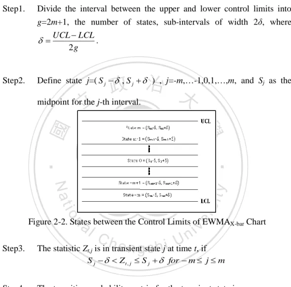
(16) 2.4 Calculation of Average Run Length for the EWMAX-bar Chart We used the Markov chain to calculate ARL, referring to Saccucci and Lucas (1990). The procedure is as follows: Step1.. Divide the interval between the upper and lower control limits into g=2m+1, the number of states, sub-intervals of width 2δ, where UCL LCL . 2g. Step2.. Define state j=( S j , S j ) , j=-m,…-1,0,1,…,m, and Sj as the. 政 治 大 midpoint for the j-th interval. 立. ‧. ‧ 國. 學 er. io. sit. y. Nat. al. v. n. Figure 2-2. States between the Control Limits of EWMAX-bar Chart. Ch. engchi. i n U. Step3.. The statistic Zt,j is in transient state j at time t, if S j Z t , j S j for m j m. Step4.. The transition probability matrix for the transient state is. R [ pt1,t ( jk )] , j, k=-m,…, -1, 0, 1,…, m where pt 1,t ( jk ) P( S k Z t ,k S k | S j Z t 1, j S j ) P( S k Z t ,k S k | Z t 1, j S j ) P( S k X t ,k (1 ) Z t 1,k S k | Z t 1, j S j ) P(. ( S k ) (1 ) S j. . 6. Xt . ( S k ) (1 ) S j. . ).
(17) Step5.. Assume. that. the. process. begins. from. state. 0;. thus,. m m pzs (0,0,...,0,1, 0,...,0,0) .. Step6. (1) Calculate zero-state ARL0. 1 ARL0 pTzs I RI 1. (2-3). where RI is the transition probability matrix calculated by in-control gamma distribution, I is the g*g dimension identity matrix and 1 is the g*1 dimension vector with all components are 1. (2) Calculate zero-state ARL1. 立. 治 政 1 ARL p I R 大 T zs. 1. 1. (2-4). O. ‧. ‧ 國. 學. where RO is the transition probability matrix calculated by out-of-control gamma distribution, I is the g*g dimension identity matrix and 1 is the g*1 dimension vector with all components are 1.. sit. y. Nat. 2.5 Determining Control Limit Coefficient on EWMAX-bar Control Chart under Different n and λ. n. al. er. io. We determine the control limit coefficient by using the following step:. Ch. i n U. v. Step1.. Determine the UCL coefficient (L1) of the EWMAX-bar control chart. With n, aI, bI, and λ, let LCL=0 and ARL0=740 to solve L1 using the routine “uniroot” in the R program. Hence, UCL is determined.. Step2.. Determine the LCL coefficient (L2) of the EWMAX-bar control chart. With UCL, let ARL0=370 to solve L2 by using the routine “uniroot” in. engchi. the R program. Hence, the economic EWMAX-bar control chart is constructed. We then obtain a combination (λ, L1, L2) for given n, aI, bI, and λ with ARL0=370.. 7.
(18) Table 2-1. The solved L1 and L2 under various combinations of λ and n for aI=1.5, bI=2, ARL0=370 and g=301 n. 2. (L1,L2). 3. 4. 5. 6. 7. 8. 9. 10. λ 0.05. 2.666. 2.300. 2.623. 2.346. 2.597. 2.373. 2.580. 2.392. 2.567. 2.406. 2.557. 2.417. 2.549. 2.425. 2.542. 2.433. 2.537. 2.439. 0.1. 3.075. 2.339. 3.001. 2.407. 2.957. 2.449. 2.927. 2.477. 2.905. 2.498. 2.888. 2.515. 2.874. 2.528. 2.863. 2.539. 2.853. 2.549. 0.2. 3.506. 2.280. 3.383. 2.379. 3.310. 2.441. 3.260. 2.484. 3.224. 2.516. 3.195. 2.541. 3.172. 2.561. 3.153. 2.578. 3.138. 2.592. 0.3. 3.785. 2.185. 3.622. 2.308. 3.526. 2.384. 3.460. 2.438. 3.411. 2.478. 3.374. 2.509. 3.344. 2.535. 3.319. 2.557. 3.298. 2.575. 0.4. 3.996. 2.087. 3.801. 2.228. 3.685. 2.316. 3.606. 2.378. 3.548. 2.425. 3.503. 2.462. 3.466. 2.493. 3.436. 2.518. 3.411. 2.539. 0.5. 4.165. 1.991. 3.943. 2.147. 3.811. 2.245. 3.721. 2.315. 3.654. 2.368. 3.603. 2.410. 3.561. 2.444. 3.527. 2.473. 3.498. 2.497. 0.6. 4.300. 1.899. 4.057. 2.067. 3.912. 2.175. 3.813. 2.252. 3.739. 2.310. 3.682. 2.356. 3.637. 2.394. 3.599. 2.426. 3.567. 2.453. 0.7. 4.404. 1.811. 4.146. 1.991. 3.990. 2.108. 3.884. 0.8. 4.480. 1.728. 4.210. 1.920. 4.048. 2.045. 3.937. 0.9. 4.527. 1.653. 4.250. 1.859. 4.084. 1.993. 立. 3.969. 政 治 大 2.191. 3.806. 2.254. 3.745. 2.304. 3.696. 2.346. 3.655. 2.380. 3.620. 2.410. 2.135. 3.855. 2.203. 3.791. 2.257. 3.739. 2.302. 3.696. 2.339. 3.660. 2.371. 2.090. 3.885. 2.163. 3.819. 2.221. 3.766. 2.268. 3.722. 2.308. 3.685. 2.342. ‧ 國. 學. We plot L1 or L2 at various n, which is shown in Figs. 2-3 and 2-4, respectively. The value of L1 decrease and L2 almost increase as n increase or λ decrease.. ‧. n. er. io. sit. y. Nat. al. Ch. engchi. i n U. v. Figure 2-3. The Value of L1 under Various n at ARL0=370, aI =1.5, bI =2 and g=301. Figure 2-4. The Value of L2 under Various n at ARL0=370, aI =1.5, bI =2 and g=301. 8.
(19) Table 2-2. The solved L1 and L2 under various combinations of λ and n for aI =24.349, bI=0.205, ARL0=370 and g=301 n. 2. (L1,L2). 3. 4. 5. 6. 7. 8. 9. 10. λ 0.05. 2.496. 2.483. 2.491. 2.488. 2.491. 2.488. 2.494. 2.486. 2.497. 2.482. 2.502. 2.478. 2.507. 2.473. 2.512. 2.468. 2.518. 2.462. 0.1. 2.775. 2.626. 2.758. 2.643. 2.749. 2.653. 2.743. 2.659. 2.739. 2.662. 2.737. 2.665. 2.735. 2.667. 2.734. 2.668. 2.734. 2.669. 0.2. 3.007. 2.713. 2.978. 2.741. 2.961. 2.758. 2.949. 2.770. 2.941. 2.778. 2.934. 2.784. 2.929. 2.789. 2.925. 2.794. 2.921. 2.797. 0.3. 3.126. 2.729. 3.088. 2.766. 3.065. 2.787. 3.049. 2.802. 3.038. 2.813. 3.029. 2.822. 3.022. 2.829. 3.016. 2.834. 3.011. 2.839. 0.4. 3.205. 2.722. 3.158. 2.765. 3.130. 2.791. 3.112. 2.809. 3.098. 2.822. 3.087. 2.833. 3.078. 2.841. 3.071. 2.848. 3.065. 2.854. 0.5. 3.262. 2.705. 3.208. 2.755. 3.176. 2.784. 3.155. 2.805. 3.139. 2.820. 3.127. 2.832. 3.117. 2.841. 3.108. 2.849. 3.101. 2.856. 0.6. 3.305. 2.684. 3.246. 2.739. 3.211. 2.772. 3.187. 2.795. 3.169. 2.812. 3.155. 2.825. 3.144. 2.835. 3.135. 2.844. 3.127. 2.852. 0.7. 3.338. 2.663. 3.274. 2.722. 3.236. 2.758. 3.210. 0.8. 3.363. 2.643. 3.295. 2.707. 3.255. 2.746. 3.227. 0.9. 3.378. 2.628. 3.308. 2.695. 3.266. 2.736. 立. 3.238. 政 治 大 2.783. 3.191. 2.801. 3.176. 2.816. 3.164. 2.827. 3.154. 2.837. 3.146. 2.845. 2.772. 3.207. 2.791. 3.191. 2.807. 3.179. 2.819. 3.168. 2.829. 3.159. 2.838. 2.763. 3.217. 2.784. 3.201. 2.800. 3.188. 2.813. 3.177. 2.823. 3.168. 2.832. ‧ 國. 學. We plot L1 or L2 at various n, which is shown in Figs. 2-5 and 2-6, respectively. The value of L1 decrease and L2 almost increase as n increase or λ decrease.. ‧. n. er. io. sit. y. Nat. al. Ch. engchi. i n U. v. Figure 2-5. The Value of L1 under Various n at ARL0=370, aI =24.349, bI =0.205 and g=301. Figure 2-6. The Value of L2 under Various n at ARL0=370, aI =24.349, bI =0.205 and g=301 9.
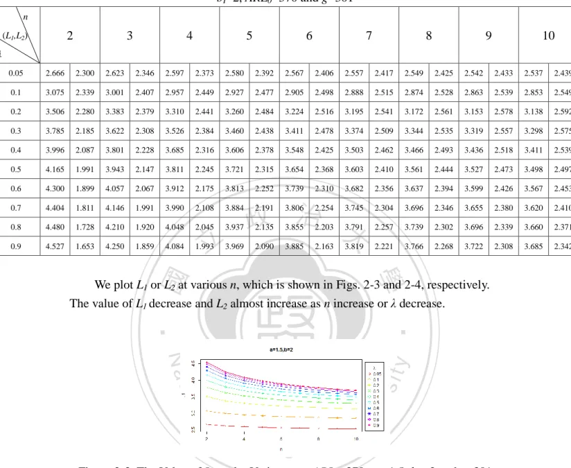
(20) Table 2-3. The solved L1 and L2 under various combinations of λ and n for aI =1, bI=0.202, ARL0=370 and g=301 n. 2. (L1,L2). 3. 4. 5. 6. 7. 8. 9. 10. λ 0.05. 2.718. 2.246. 2.666. 2.300. 2.635. 2.333. 2.613. 2.356. 2.597. 2.373. 2.585. 2.386. 2.575. 2.397. 2.567. 2.406. 2.560. 2.413. 0.1. 3.165. 2.259. 3.075. 2.339. 3.021. 2.389. 2.985. 2.423. 2.957. 2.449. 2.936. 2.468. 2.919. 2.485. 2.905. 2.498. 2.893. 2.510. 0.2. 3.657. 2.163. 3.506. 2.280. 3.416. 2.352. 3.355. 2.403. 3.310. 2.441. 3.275. 2.471. 3.247. 2.495. 3.224. 2.516. 3.204. 2.533. 0.3. 3.984. 2.044. 3.785. 2.185. 3.666. 2.274. 3.585. 2.337. 3.526. 2.384. 3.479. 2.422. 3.442. 2.452. 3.411. 2.478. 3.385. 2.500. 0.4. 4.234. 1.928. 3.996. 2.087. 3.854. 2.189. 3.757. 2.261. 3.685. 2.316. 3.630. 2.360. 3.585. 2.395. 3.548. 2.425. 3.517. 2.451. 0.5. 4.434. 1.818. 4.165. 1.991. 4.003. 2.104. 3.893. 2.184. 3.811. 2.245. 3.748. 2.294. 3.697. 2.334. 3.654. 2.368. 3.619. 2.397. 0.6. 4.594. 1.714. 4.300. 1.899. 4.123. 2.020. 4.001. 2.108. 3.912. 2.175. 3.842. 2.229. 3.786. 2.273. 3.739. 2.310. 3.700. 2.342. 0.7. 4.717. 1.616. 4.404. 1.811. 4.216. 1.941. 4.086. 0.8. 4.806. 1.523. 4.480. 1.728. 4.283. 1.866. 4.148. 0.9. 4.860. 1.437. 4.527. 1.653. 4.325. 1.801. 立. 4.186. 政 治 大 2.035. 3.990. 2.108. 3.916. 2.166. 3.856. 2.214. 3.806. 2.254. 3.764. 2.289. 1.967. 4.048. 2.045. 3.970. 2.108. 3.907. 2.159. 3.855. 2.203. 3.810. 2.241. 1.909. 4.084. 1.993. 4.003. 2.061. 3.939. 2.116. 3.885. 2.163. 3.839. 2.203. ‧ 國. 學. We plot L1 or L2 at various n, which is shown in Figs. 2-7 and 2-8, respectively. The value of L1 decrease and L2 almost increase as n increase or λ decrease.. ‧. n. er. io. sit. y. Nat. al. Ch. engchi. i n U. v. Figure 2-7. The Value of L1 under Various n at ARL0=370, aI =1, bI =0.202 and g=301. Figure 2-8. The Value of L2 under Various n at ARL0=370, aI =1, bI =0.202 and g=301. 10.
(21) 2.6 Determining the Best λ in the EWMAX-bar Chart under Different δ1, δ2 and n We use L1 and L2 in Table 2-1, to ensure that ARL0=370, The ARL1 under various λ and n are illustrated in Table 2-4 at aI =1.5, bI =2, δ1=0.1, δ2=0.05, and g=301. Table 2-4. The Value of ARL1 under Various n and λ at aI =1.5, bI =2, δ1=0.1, δ2=0.05, g=301 and ARL0=370 n ARL1. 2. 3. 4. 5. 6. 7. 8. 9. 10. λ. 0.05. 134.33 102.74. 83.83. 71.23. 62.22. 55.46. 50.18. 45.96. 42.49. 0.1. 173.51 133.99 108.98. 91.77. 79.25. 69.75. 62.31. 56.33. 51.43. 0.2. 228.61 184.38 153.69 131.23 114.14 100.73. 89.95. 81.12. 73.76. 0.3. 265.27 222.07 190.04. 117.28 106.44. 97.25. 0.4. 291.10 250.95 219.65 194.64 174.24 157.33 143.07 130.93 120.47. 0.5. 309.69 273.30 243.80 219.45 199.06 181.78 166.92 154.06 142.82. 0.6. 323.11 290.50 263.27 240.26 220.54 203.48 188.59 175.50 163.88. 0.7. 332.53 303.46 278.69 257.32 238.71 222.34 207.83 194.89 183.28. 0.8. 338.65 312.69 290.33 270.79 253.54 238.16 224.36 211.91 200.61. 0.9. 341.63 318.19 298.07 280.41 264.68 250.56 237.74 226.05 215.36. 立. 治 政 大 165.42 145.97 130.24. ‧. ‧ 國. 學. sit. y. Nat. n. al. er. io. According to Table 2-4, to minimize ARL1, 0.05 is the best λ for n=2,…, 10.. Ch. engchi. 11. i n U. v.
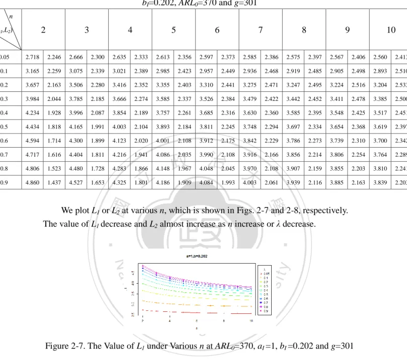
(22) We use L1 and L2 in Table 2-2, to ensure that ARL0=370, The ARL1 under various λ and n are illustrated in Table 2-5 at aI =24.349, bI =0.205, δ1=0.919, δ2=0.06, and g=301. Table 2-5. The Value of ARL1 under Various n and λ at aI =24.349, bI =0.205, δ1=0.919, δ2=0.06, g=301 and ARL0=370 n ARL1. 2. 3. 4. 5. 6. 7. 8. 9. 10. λ. 0.05. 4.23 3.47 3.03 2.74 2.52 2.35 2.23 2.13 2.06. 0.1. 3.56 2.89 2.52 2.28 2.12 2.00 1.91 1.83 1.76. 0.2. 3.07 2.45 2.12 1.91 1.75 1.63 1.52 1.43 1.34. 0.3. 2.89 2.25 1.92 1.70 1.54 1.42 1.32 1.24 1.18. 0.4. 2.85 2.15. 0.5. 2.89 2.11 1.73 1.51 1.36 1.25 1.17 1.12 1.08. 0.6. 3.01 2.12 1.70 1.47 1.32 1.21 1.14 1.10 1.06 3.23 2.17 1.71 1.45 1.30 1.20 1.13 1.08 1.05 3.54 2.27 1.74 1.46 1.29 1.19 1.12 1.08 1.05. ‧. 0.9. ‧ 國. 0.8. 1.16 1.11. 學. 0.7. 立. 治 政 大1.23 1.80 1.58 1.43 1.31. 3.97 2.44 1.81 1.49 1.30 1.19 1.12 1.07 1.05. y. Nat. sit. n. al. er. io. According to Table 2-5, we find the best combination of λ and n with minimum ARL1. They are summarized in Table 2-6.. i n U. v. Table 2-6. Combination of λ, n, L1 and L2 with Minimum ARL1 n. 2. 3. λ. 0.4. 0.5. Ch. e n g5c h i 6. 4. 0.6. L1 3.205 3.208 3.211. 0.7 3.21. 0.8. 0.8. λ. 8 0.8. 9 0.9. 0.9. 10 0.7. 0.8. 0.9. L1 3.179 3.188 3.177 3.146 3.159 3.168 L2 2.819 2.813 2.823 2.845 2.838 2.832. 12. 0.9. 3.207 3.191 3.201. L2 2.722 2.755 2.772 2.783 2.791 2.807 n. 7. 2.8.
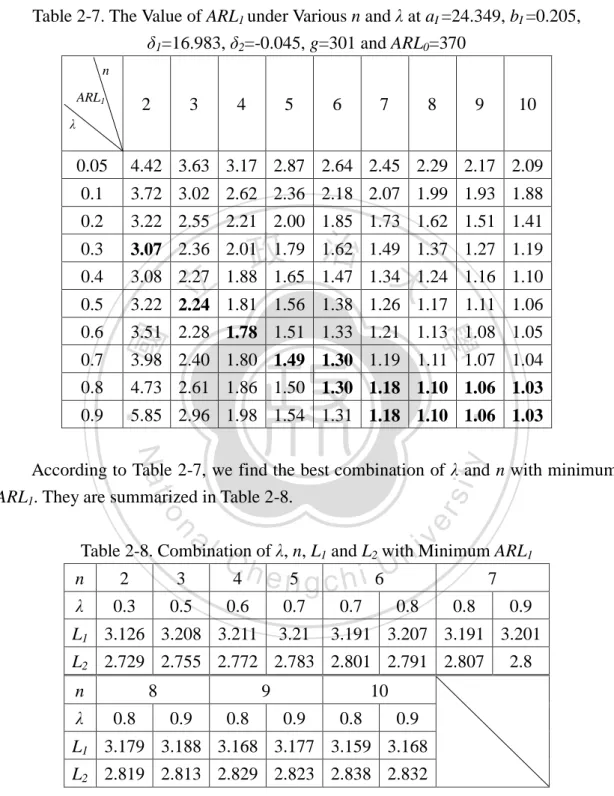
(23) We use L1 and L2 in Table 2-2, to ensure that ARL0=370, The ARL1 under various λ and n are illustrated in Table 2-7 at aI =24.349, bI =0.205, δ1=16.983, δ2=-0.045, and g=301. Table 2-7. The Value of ARL1 under Various n and λ at aI =24.349, bI =0.205, δ1=16.983, δ2=-0.045, g=301 and ARL0=370 n ARL1. 2. 3. 4. 5. 6. 7. 8. 9. 10. λ. 0.05. 4.42 3.63 3.17 2.87 2.64 2.45 2.29 2.17 2.09. 0.1. 3.72 3.02 2.62 2.36 2.18 2.07 1.99 1.93 1.88. 0.2. 3.22 2.55 2.21 2.00 1.85 1.73 1.62 1.51 1.41. 0.3. 3.07 2.36 2.01 1.79 1.62 1.49 1.37 1.27 1.19. 0.4. 3.08 2.27. 0.5. 3.22 2.24 1.81 1.56 1.38 1.26 1.17 1.11 1.06. 0.6. 3.51 2.28 1.78 1.51 1.33 1.21 1.13 1.08 1.05 3.98 2.40 1.80 1.49 1.30 1.19 1.11 1.07 1.04 4.73 2.61 1.86 1.50 1.30 1.18 1.10 1.06 1.03. ‧. 0.9. ‧ 國. 0.8. 1.16 1.10. 學. 0.7. 立. 治 政 大1.24 1.88 1.65 1.47 1.34. 5.85 2.96 1.98 1.54 1.31 1.18 1.10 1.06 1.03. y. Nat. sit. n. al. er. io. According to Table 2-7, we find the best combination of λ and n with minimum ARL1. They are summarized in Table 2-8.. i n U. v. Table 2-8. Combination of λ, n, L1 and L2 with Minimum ARL1 n. 2. 3. Ch. λ. 0.3. 0.5. 0.6. 4. e n5 g c h i 6 0.7. L1 3.126 3.208 3.211. 3.21. 0.7. 0.8. 7 0.8. 3.191 3.207 3.191 3.201. L2 2.729 2.755 2.772 2.783 2.801 2.791 2.807 n λ. 8 0.8. 9 0.9. 0.8. 10 0.9. 0.8. 0.9. L1 3.179 3.188 3.168 3.177 3.159 3.168 L2 2.819 2.813 2.829 2.823 2.838 2.832. 13. 0.9 2.8.
(24) We use L1 and L2 in Table 2-2, to ensure that ARL0=370, The ARL1 under various λ and n are illustrated in Table 2-9 at aI =24.349, bI =0.205, δ1=-8.741, δ2=0.123, and g=301. Table 2-9. The Value of ARL1 under Various n and λ at aI =24.349, bI =0.205, δ1=-8.741, δ2=0.123, g=301 and ARL0=370 n ARL1. 2. 3. 4. 5. 6. 7. 8. 9. 10. λ. 0.05. 68.69 57.75 50.29 44.84 40.66 37.35 34.65 32.40 30.50. 0.1. 64.82 55.51 48.76 43.62 39.58 36.30 33.60 31.32 29.38. 0.2. 60.84 53.73 48.18 43.71 40.04 36.98 34.37 32.12 30.18. 0.3. 58.58 52.85 48.17 44.27 40.96 38.12 35.66 33.51 31.60. 0.4. 57.15. 0.5. 56.21. 0.6. 55.61 52.15 49.11 46.39 43.96 41.76 39.76 37.94 36.27. 0.7. 55.23 52.26 49.60 47.20 45.00 43.00 41.16 39.46 37.89. 0.8. 54.98 52.46 50.15 48.02 46.06 44.25 42.57 41.00 39.54. 0.9. 54.83 52.70 50.71 48.86 47.12 45.50 43.98 42.54 41.20. 治 政 大 52.38 48.36 44.92 41.93 39.32 52.17立 48.68 45.63 42.93 40.53. 37.02 34.96 33.13 38.38 36.44 34.68. ‧. ‧ 國. 學. y. Nat. sit. n. al. er. io. According to Table 2-9, we find the best combination of λ and n with minimum ARL1. They are summarized in Table 2-10.. i n U. v. Table 2-10. Combination of λ, n, L1 and L2 with Minimum ARL1 n. 2. 3. 4. λ. 0.9. 0.6. 0.3. Ch. e n g6c h i 7. 5. 0.1. 0.1. 0.1. 8. 9. 10. 0.1. 0.1. 0.1. L1 3.378 3.246 3.065 2.494 2.497 2.502 2.507 2.512 2.518 L2 2.628 2.739 2.787 2.486 2.482 2.478 2.473 2.468 2.462. 14.
(25) We use L1 and L2 in Table 2-2, to ensure that ARL0=370, The ARL1 under various λ and n are illustrated in Table 2-11 at aI =24.349, bI =0.205, δ1=9.452, δ2=-0.097, and g=301. Table 2-11. The Value of ARL1 under Various n and λ at aI =24.349, bI =0.205, δ1=9.452, δ2=-0.097, g=301 and ARL0=370 n ARL1. 2. 3. 4. 5. 6. 7. 8. 9. 10. λ. 0.05. 5.26 4.29 3.73 3.34 3.09 2.95 2.80 2.62 2.42. 0.1. 4.38 3.53 3.09 2.79 2.52 2.30 2.14 2.06 2.02. 0.2. 3.70 2.94 2.50 2.23 2.08 2.01 1.96 1.90 1.82. 0.3. 3.44 2.65 2.27 2.06 1.94 1.83 1.70 1.56 1.43. 0.4. 3.35 2.52. 0.5. 3.41 2.47 2.05 1.79 1.58 1.41 1.27 1.17 1.10. 0.6. 3.62 2.46 1.97 1.67 1.45 1.30 1.18 1.11 1.06 4.04 2.52 1.92 1.58 1.37 1.22 1.13 1.07 1.04 4.83 2.69 1.92 1.54 1.32 1.18 1.10 1.05 1.03. ‧. 0.9. ‧ 國. 0.8. 1.30 1.20. 學. 0.7. 立. 治 政 大1.44 2.14 1.93 1.75 1.59. 6.33 3.05 2.00 1.53 1.29 1.16 1.08 1.04 1.02. y. Nat. sit. n. al. er. io. According to Table 2-11, we find the best combination of λ and n with minimum ARL1. They are summarized in Table 2-12.. i n U. v. Table 2-12. Combination of λ, n, L1 and L2 with Minimum ARL1 n. 2. 3. λ. 0.4. 0.6. 4 0.7. Ch 0.8. e n5 g c h6 i 0.9. 0.9. 7. 8. 9. 10. 0.9. 0.9. 0.9. 0.9. L1 3.205 3.246 3.236 3.255 3.238 3.217 3.201 3.188 3.177 3.168 L2 2.722 2.739 2.758 2.746 2.763 2.784. 15. 2.8. 2.813 2.823 2.832.
(26) We use L1 and L2 in Table 2-3, to ensure that ARL0=370, The ARL1 under various λ and n are illustrated in Table 2-13 at aI =1, bI =0.202, δ1=0, δ2=0.077, and g=301. Table 2-13. The Value of ARL1 under Various n and λ at aI =1, bI =0.202, δ1=0, δ2=0.077, g=301 and ARL0=370 n ARL1. 2. 3. 4. 5. 6. 7. 8. 9. 10. λ. 0.05. 24.93 18.87 15.60 13.52 12.06 10.97 10.12. 9.44. 8.87. 0.1. 27.11 19.52 15.58 13.15 11.49 10.29. 9.37. 8.64. 8.05. 0.2. 34.26 23.62 18.08 14.72 12.48 10.89. 9.70. 8.78. 8.05. 0.3. 42.05 28.87 21.78 17.43 14.52 12.45 10.92. 9.74. 8.80. 0.4. 49.62 34.51 26.06 20.75 17.15 14.57 12.65 11.17 10.00. 0.5. 56.67. 0.6. 63.06. 0.7. 68.68 51.00 39.99 32.52 27.16 23.15 20.06 17.61 15.64. 0.8. 73.50 55.80 44.46 36.58 30.83 26.45 23.03 20.30 18.07. 0.9. 77.43 60.02 48.58 40.48 34.45 29.80 26.12 23.14 20.70. 政 治 大 40.21 30.64 24.47 20.21 17.12 45.76立 35.34 28.44 23.58 20.00. 14.79 12.99 11.56 17.28 15.15 13.45. ‧. ‧ 國. 學. er. io. sit. y. Nat. According to Table 2-13, we find the best combination of λ and n with minimum ARL1. They are summarized in Table 2-14. Table 2-14. Combination of λ, n, L1 and L2 with Minimum ARL1. n. al. n. 2. 3. 4. λ. 0.05. 0.05. 0.1. Ch 5. 0.1. 6. 7. e 0.1 hi n g c 0.1. i n U 8. 0.1. v. 9 0.1. 10 0.1. 0.2. L1 2.718 2.666 3.021 2.985 2.957 2.936 2.919 2.905 2.983 3.204 L2 2.246. 2.3. 2.389 2.423 2.449 2.468 2.485 2.498. 16. 2.51. 2.533.
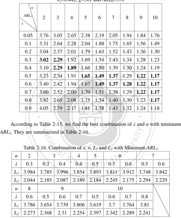
(27) We use L1 and L2 in Table 2-3, to ensure that ARL0=370, The ARL1 under various λ and n are illustrated in Table 2-15 at aI =1, bI =0.202, δ1=0, δ2=0.442, and g=301. Table 2-15. The Value of ARL1 under Various n and λ at aI =1, bI =0.202, δ1=0, δ2=0.442, g=301 and ARL0=370 n ARL1. 2. 3. 4. 5. 6. 7. 8. 9. 10. λ. 0.05. 3.76 3.05 2.65 2.38 2.19 2.05 1.94 1.84 1.76. 0.1. 3.31 2.64 2.28 2.04 1.88 1.75 1.65 1.56 1.49. 0.2. 3.04 2.37 2.01 1.79 1.63 1.52 1.43 1.36 1.30. 0.3. 3.02 2.29 1.92 1.69 1.54 1.43 1.34 1.28 1.23. 0.4. 3.10 2.29 1.89 1.66 1.50 1.39 1.30 1.24 1.19. 0.5. 3.23 2.34. 0.6. 3.40. 0.7. 3.60 2.52 2.00 1.70 1.51 1.38 1.29 1.22 1.17. 1.22 1.17. 1.67 1.49 1.37 1.28 1.22 1.17. ‧ 國. 0.9. 立 1.94 2.42. 學. 0.8. 政 治 大 1.91 1.65 1.49 1.37 1.29. 3.82 2.65 2.08 1.75 1.54 1.40 1.30 1.23 1.17 4.05 2.79 2.17 1.81 1.58 1.43 1.32 1.24 1.18. ‧. er. io. sit. y. Nat. According to Table 2-15, we find the best combination of λ and n with minimum ARL1. They are summarized in Table 2-16. Table 2-16. Combination of λ, n, L1 and L2 with Minimum ARL1. al. n. n. 2. λ. 0.3. 3 0.3. 0.4. Ch. 4. 5. i n U. e n g0.5c h i0.5. 0.4. 6. v. 0.6. 7 0.5. 0.6. L1 3.984 3.785 3.996 3.854 3.893 3.811 3.912 3.748 3.842 L2 2.044 2.185 2.087 2.189 2.184 2.245 2.175 2.294 2.229 n. 8. λ. 0.6. 9 0.5. 0.6. 10 0.7. 0.5. L1 3.786 3.654 3.739 3.806 3.619 L2 2.273 2.368. 2.31. 0.6. 0.7. 0.8. 3.7. 3.764. 3.81. 2.254 2.397 2.342 2.289 2.241. 17.
(28) We summarize all the best λ under various n in Tables 2-4, 2-5,…, 2-16 as follows: Table 2-17. The Best λ in Tables 2-4, 2-5,…, 2-16.. 2. 0.1. 0.05. shift scale. 0.114. 1.058 0.05 0.05 0.05 0.05 0.05 0.05 0.05 0.05 0.05 1.317. 24.349 0.205 16.983 -0.045. 1.603. 1.017. 24.349 0.205 -8.741. 0.123. 0.126. 24.349 0.205. -0.097 -1.326 0.621 0.381. 4. 5. 6. 7. 8. 2.188. 0.4. 0.5. 0.6. 政 治 大 1.281 0.9 0.6 0.3 0.3. 0.5. 0.6. 0.6. 0.7, 0.8. 1.381 0.05 0.05. 0.1. io. 0.4. 0.3. 0.3, 0.4. n. al. 3.188. Ch. 10. 0.8, 0.9. 0.9. 0.7, 0.8, 0.9. 0.7. 0.8. 0.8, 0.9. 0.7. 0.7, 0.8. 0.8, 0.9. 0.8, 0.9. 0.8, 0.9. 0.8, 0.9. 0.1. 0.1. 0.1. 0.1. 0.1. 0.1. 0.9. 0.9. 0.9. 0.9. 0.9. 0.9. 0.1. 0.1. 0.1. 0.1. 0.1. 0.6. 0.5, 0.6, 0.7. 0.4. 0.5. 0.5, 0.6. 0.5, 0.6. i n U. v. In Table 2-17, the value of the mean shift scale and the value of the s.d. shift scale are calculated as follow: mean shift scale =. 9. The best λ. er. 0.442. 3. ‧. 0. 0.077. 2. 學. 0.202. 0. 立. Nat. 1. 0.202. 9.452. 0.06. shift scale. 1.685. 1. 0.919. δ2. ‧ 國. 24.349 0.205. δ1. y. 1.5. bI. s.d.. sit. aI. n. mean. engchi. aO bO aI bI aI bI2. and s.d. shift scale =. aO bO2 a I bI2. According to Table 2-17, n significantly affects the value of the best λ when both the mean shift scale and the s.d. shift scale have a large value. In addition, the larger the mean shift scale or s.d. shift scale, the larger the value of the best λ.. 18. 0.1, 0.2 0.5, 0.6, 0.7, 0.8.
(29) CHAPTER 3. DERIVATION OF THE PROFIT MODEL WITHOUT PRODUCER INSPECTION. 3.1 Derivation of Expected Cycle Time In Sections 3.1 and 3.2, we derive the profit model, referring to Panagos, Heikes, and Montgomery (1985). We begin with the following assumptions: (1) The process has a single assignable cause. The time until occurrences of the assignable cause is the exponential distribution with θ mean per unit time. (2) The process starts in the in-control state. (3) When the assignable cause occurs, both parameters of gamma distribution a and b shift to a+δ1 and b+δ2, respectively. (4) For every h unit time, a sample size n is taken, and its average is plotted on the EWMAX-bar control chart. (5) The manufacturing continues when the assignable cause is searched.. 立. 政 治 大. ‧. ‧ 國. 學. n. al. er. io. sit. y. Nat. Similar to Figure 3-1, the cycle starts in the in-control state, and then the assignable cause occurs, becoming an out-of-control state, an EWMAX-bar statistic falls outside the control limits, the result is tested and interpreted, and an assignable cause is then found and repaired.. i n U. v. Because the time until an assignable cause occurrence is the exponential distribution with θ mean per unit time, the expected time of the in-control state is 1/θ.. Ch. engchi. h h 2 . The 2 12 expected time of the out-of-control state is h/(1-β), where 1-β is the power of the control chart. The time to test and interpret the results is equal to e*n and the time to find and repair an assignable cause is equal to D.. The expected time of shift occurrence in the sampling time h is . In-control. Out-of-control. Assignable cause. τ. h/(1-β)-τ. e*n. 1/θ Figure 3-1. Continuous Process Cycle. 19. D.
(30) Because we use the EWMAX-bar control chart, we calculate α and β as follows: 1 (3-1) ARL 0. 1. 1 ARL1. (3-2). where ARL0 and ARL1 are calculated using Equations 2-3 and 2-4, respectively. Hence, the expected cycle time is ET . 1. . h( ARL1 . 1 h ) en D 2 12. (3-3). 3.2 Derivation of the Expected Cycle Profit. 政 治 大. The quality variable, which we consider, is the smaller the better; therefore, we use the quadratic Taguchi loss function, as follows:. 立. ‧ 國. (3-4). 學. L kc X 2. where X >0 is the quality variable and kc is the coefficient of loss function.. ‧. . (3-5). io. er. 2. y. . E L kc E X Var X . sit. Nat. If the producer decides not to inspect products, then the expected cost per unit item using the quadratic Taguchi loss function is. al. n. v i n Ch engchi U k E X Var X k a b a b . Hence, in the in-control state, the expected cost per unit item is. I. 2. c. I. I. c. 2 2 I I. 2 I I. (3-6). and, in the out-of-control state, the expected cost per unit item is. . . O kc E X O Var X O kc aI 1 bI 2 aI 1 bI 2 2. 2. 2. 2. . (3-7). Assume that the sale price for conformable product is PC, but the sale price for unconformable product is PU, and PC >PU . We let the sale price for product without inspection is PW PC P X I USL PU P X I USL (3-8). 20.
(31) Hence, in the in-control state, the expected net profit per unit time is EPI PW I R. (3-9). where R is the number of products per unit time. Similarly, in the out-of-control state, the expected net profit per unit time is (3-10) EPO PW O R We include the cost of investigating a false alarm which is T, the cost of taking a sample, is s0+s1*n, and the cost of finding and repairing an assignable cause which is W. Hence, the expected cycle profit is T 1 1 h ( s s n) ET EP EPI W (3-11) EPO h( ARL1 ) en D 0 1 hARL0 h 2 12 . 立. 政 治 大 EAP . 學. ‧ 國. Therefore, the expected profit per unit time is. EP ET. (3-12). ‧. sit. y. Nat. 3.3 Determining Optimum Design Parameters of the Economic EWMAX-bar Control Chart. n. al. er. io. The procedure to determine n*, h*, and (λ, L1, L2) of the economic EWMAX-bar control chart without producer inspection is as follows:. Ch. engchi. i n U. v. Step1.. Let n=2.. Step2.. Determine the UCL coefficient (L1) of the EWMAX-bar control chart. With a, b, and λ, let LCL=0 and ARL0=740 to solve L1 by using the routine “uniroot” in the R program. Hence, UCL is determined.. Step3.. Determine the LCL coefficient (L2) of the EWMAX-bar control chart. With UCL, let ARL0=370 to solve L2 using the routine “uniroot” in the R program. Hence, the economic EWMAX-bar control chart is constructed.. 21.
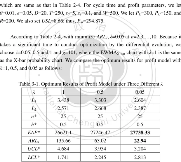
(32) Step4.. We use the routine “DEoptim” of the R program for global optimization by differential evolution to maximize EAP, subject to 0.5≦h≦8. Hence, h* is determined. If EAP(n+1) is greater than EAP(n), then we choose EAP(n+1) to become EAP*.. Step5.. Let n=n+1, 3≦n≦25. Proceed to Step2.. 3.4 An Example For the gamma distribution parameters, we let aI =1.5, bI =2, δ1=0.1, and δ2=0.05 which are same as that in Table 2-4. For cycle time and profit parameters, we let θ=0.01, e=0.05, D=20, T=250, s0=5, s1=0.1, and W=500. We let PC=300, PU=150, and R=200. We also set USL=8.66; thus, PW=294.875.. 政 治 大 According to Table 2-4, with minimize ARL , λ=0.05 at n=2,3,…,10. Because it 立 takes a significant time to conduct optimization by the differential evolution, we 1. ‧ 國. 學. choose λ=0.05, 0.5 and 1 and g=101, where the EWMAX-bar chart with λ=1 is the same as the X-bar probability chart. We compare the optimum results for profit model with. ‧. λ=1, 0.5, and 0.05 as follows:. n* h*. 3.303. a2.571 l 25 C h. 2.668. 0.5. e n g c0.5h i U 25. y. 3.438. 0.05. sit. 0.5. n. L2. io. L1. 1. 2.604. er. λ. Nat. Table 3-1. Optimum Results of Profit Model under Three Different λ. v ni. 2.387 25 0.5. EAP*. 26621.1. 27246.47. 27738.33. ARL1. 135.66. 63.02. 22.94. UCL*. 4.684. 3.934. 3.204. LCL*. 1.741. 2.245. 2.813. According to Table 3-1, n* and h* are the same in three types of optimum results, but we have the largest EAP*, the smallest ARL1, and the narrowest chart when we use the economic EWMAX-bar chart with λ=0.05. The table shows that λ affects the optimum result significantly. Therefore, we suggest that the producer use the economic EWMAX-bar chart with λ=0.05 and take 25 samples every 0.5 unit time to obtain 27738.3 profits per unit time. 22.
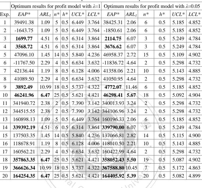
(33) 3.5 Sensitivity Analysis and Comparing the Results with λ=1 In sensitivity analysis, we choose two levels of parameters in orthogonal arrays L20(219), which is designed by Plackett and Burman (1946), as follows: Table 3-2. Level of Parameters kc, A, IC, R. δ1. δ2. θ. e. D s0 s1 W. T. P C, PU. level 1 10,600,0.1,200 6.5 0.03 0.05 0.5 20 5 1 500 250 500,200 level 2 5,100,0.05,1000 3.5 -0.01 0.01 0.05 3 0.5 0.1 50 35 300,150 Table 3-3. Parameters for Each Experiment δ1. δ2. θ. 1. 10,600,0.1,200. 6.5 0.03 0.05 0.05 3 5. 3. 1 50 250 500,200 治 政 10,600,0.1,200 6.5 0.03 0.01 0.05 20 大 5 0.1 500 250 300,150 10,600,0.1,200立6.5 -0.01 0.05 0.5 3 0.5 0.1 50 250 300,150. 4. 10,600,0.1,200. 6.5 -0.01 0.01 0.5 20 0.5 1 500 35 300,150. 5. 10,600,0.1,200. 6.5 -0.01 0.01 0.05 3 5 0.1 500 35 500,200. 6. 10,600,0.1,200. 3.5 0.03 0.05 0.5 20 0.5 0.1 500 250 300,150. 7. 10,600,0.1,200. 3.5 0.03 0.05 0.05 3 0.5 0.1 500 35 500,200. 8. 10,600,0.1,200. 3.5 0.03 0.01 0.5 20 5. 1. 50 35 500,200. 9. 10,600,0.1,200. 3.5 -0.01 0.05 0.5 3 5. 1. 50 35 300,150. 10. 10,600,0.1,200. 3.5 -0.01 0.01 0.05 20 0.5 1. 11. 5,100,0.05,1000 6.5 0.03 0.05 0.5 3 0.5 1 500 35 500,200. 12. 5,100,0.05,1000 6.5 0.03 0.01 0.5 20 0.5 0.1 50 35 500,200. 13. 5,100,0.05,1000 6.5 0.03 0.01 0.05 3 0.5 1. 14. 5,100,0.05,1000 6.5 -0.01 0.05 0.5 20 5 0.1 50 250 500,200. 15. 5,100,0.05,1000 6.5 -0.01 0.05 0.05 20 5. 16. 5,100,0.05,1000 3.5 0.03 0.05 0.05 20 5 0.1 50 35 300,150. 17. 5,100,0.05,1000 3.5 0.03 0.01 0.5 3 5. 18. 5,100,0.05,1000 3.5 -0.01 0.05 0.05 20 0.5 1 500 250 500,200. 19. 5,100,0.05,1000 3.5 -0.01 0.01 0.5 3 5 0.1 500 250 500,200. 20. 5,100,0.05,1000 3.5 -0.01 0.01 0.05 3 0.5 0.1 50 35 300,150. D s0 s1 W. T. PC, PU. io. sit. y. ‧. Nat. n. al. e. 50 250 500,200. er. 2. ‧ 國. kc, A, IC, R. 學. Exp.. Ch. engchi. i n U. v. 50 250 300,150. 1 500 35 300,150 1 500 250 300,150. In Table 3-4, we let aI =25 and bI =0.2 to maximize EAP and determine optimum n* and h* at each experiment, subject to 2≦n≦25 and 0.5≦h≦8. The optimum results are solved as follows:. 23.
(34) Table 3-4. Optimum Results in Each Experiment n*. h*. UCL* LCL*. 1.09. 5 0.5 6.449 3.764 38425.31 2.06. 6. 0.5. 5.185 4.852. -1643.75. 1.09. 5 0.5 6.449 3.764 -1850.61 2.06. 6. 0.5. 5.185 4.852. 3. 1699.77. 4.51. 6 0.5 6.314 3.864 2114.75. 6.07. 3. 0.5. 5.249 4.784. 4. 3568.72. 4.51. 6 0.5 6.314 3.864 3676.62 6.07. 3. 0.5. 5.249 4.784. 5. 47096.10. 1.45 14 0.5 5.840 4.236 46958.37 2.72. 15. 0.5. 5.109 4.902. 6. -11767.50. 2.29. 4 0.5 6.634 3.632 -11836.72 4.64. 2. 0.5. 5.298 4.732. 7. 42136.44. 1.19. 8 0.5 6.128 4.006 41358.06 2.21. 10. 0.5. 5.143 4.885. 8. 41089.50. 2.29. 4 0.5 6.634 3.632 41050.95 4.64. 2. 0.5. 5.298 4.732. 9. 3892.49. 10.99 18 0.5 5.737 4.322 4772.07 11.46. 6. 0.5. 5.185 4.852. 10. 46241.96. 6.47 25 0.5 5.621 4.421 46298.41 5.67. 18. 0.5. 5.092 4.904. 11. 341940.72. 2.38. 2. 2. 0.5. 5.298 4.732. 12. 344515.55. 2.38. 2. 政 治 3.24 0.5 7.390 3.142 340013.93 大 0.5立 7.390 3.142 344106.96 3.24. 2. 0.5. 5.298 4.732. 13. 160898.13. 1.09. 5 0.5 6.449 3.764 160196.33 2.06. 6. 0.5. 5.185 4.852. 14. 339392.19. 4.51. 6 0.5 6.314 3.864 339790.00 6.07. 學 3. 0.5. 5.249 4.784. 15. 137503.35. 1.45 14 0.5 5.840 4.236 137066.81 2.82. 14. 0.5. 5.115 4.900. 16. 118678.91. 1.19. 8 0.5 6.128 4.006 118010.50 2.21. 10. 0.5. 5.143 4.885. 17. 160562.21. 2.29. 4 0.5 6.634 3.632 160422.99 4.64. ‧ 2. 0.5. 5.298 4.732. 18. 357863.35. 6.47 25 0.5 5.621 4.421 358052.43 5.50. 19. y. 0.5. 5.087 4.902. 19. 366626.34 10.99 18 0.5 5.737 4.322 367588.80 10.45. sit. Exp.. EAP*. 1. 39491.38. 2. ARL1 n* h* UCL* LCL*. EAP*. 7. 0.5. 5.172 4.863. 20. 164254.35. 0.5. 5.082 4.899. ‧ 國. ARL1. er. Optimum results for profit model with λ=1 Optimum results for profit model with λ=0.05. Nat. io. 6.47 25 0.5 5.621 4.421 164405.92 5.39. n. al. Ch. n U engchi. iv. 20. According to Table 3-4, at Experiment 3, 4, 9, 10, 14, 18, 19, and 20 the profit model with λ=0.05 has larger EAP* than the profit model with λ=1. We find δ1=3.5 and δ2=-0.01 are very small shift at Experiment 9, 10, 18, 19, and 20. The δ1=6.5, δ2=-0.01 and e=0.5 are small shift, but e is large at Experiments 3, 4, and 14. At Experiment 10, 18, and 20, the profit model with λ=0.05 has larger EAP* and smaller ARL1 than the profit model with λ=1. For these three experiments with larger EAP*, we find δ1=3.5 and δ2=-0.01 are very small, also e=0.05 and s0=0.5, are small. We use the optimum results for profit model with λ=0.05 in Table 3-4 to plot the response figures (from Figure 3-2. to 3-7.) and determine the parameters that affects optimum value significantly.. 24.
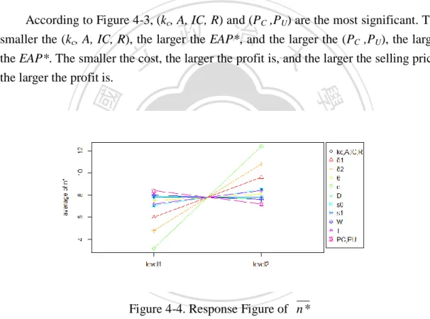
(35) Figure 3-2. Response Figure of EAP * According to Figure 3-2, (kc, A, IC, R) and (PC ,PU) are the most significant. The smaller the (kc, A, IC, R), the larger the EAP*, and the larger the (PC ,PU), the larger the EAP*. The smaller the cost, the larger the profit is, and the larger the selling price, the larger the profit is.. 立. 政 治 大. ‧. ‧ 國. 學. n. er. io. sit. y. Nat. al. Ch. engchi. i n U. v. Figure 3-3. Response Figure of n * According to Figure 3-3, δ1, δ2, and e are the most significant. The smaller the δ1, δ2 or e, the larger the n* is. The smaller shift in products necessitates more samples for testing. The term e*n causes the parameter e to affect the optimum value n* significantly.. 25.
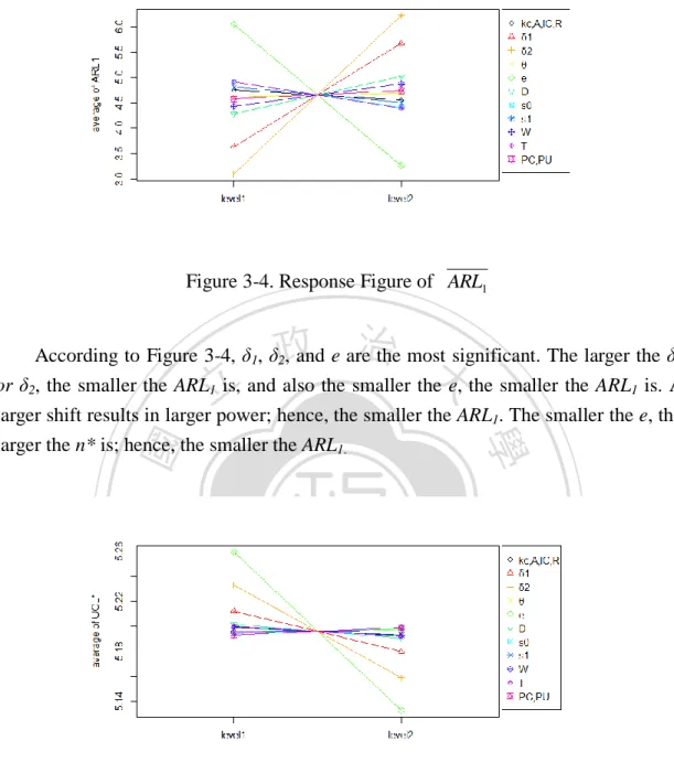
(36) Figure 3-4. Response Figure of ARL1. 政 治 大. According to Figure 3-4, δ1, δ2, and e are the most significant. The larger the δ1 or δ2, the smaller the ARL1 is, and also the smaller the e, the smaller the ARL1 is. A larger shift results in larger power; hence, the smaller the ARL1. The smaller the e, the larger the n* is; hence, the smaller the ARL1.. 立. ‧. ‧ 國. 學. n. er. io. sit. y. Nat. al. Ch. engchi. i n U. v. Figure 3-5. Response Figure of UCL * According to Figure 3-5, δ1, δ2, and e are the most significant. The smaller the δ1, δ2 or e, the smaller the UCL* is. The smaller shift in products necessitates a narrower chart to test; hence, the smaller the UCL*. The smaller the e, the larger the n* is; hence, the smaller the UCL*.. 26.
(37) Figure 3-6. Response Figure of LCL * According to Figure 3-6, δ2 and e are the most significant. The smaller the δ2 or e, the larger the LCL* is. The smaller shift in products necessitates a narrower chart to test; hence, the larger the LCL*. The smaller the e, the larger the n* is; hence, the larger the LCL*.. 立. 政 治 大. ‧ 國. 學. We use the value of EAP* of the EWMAX-bar chart with λ=0.05 minus the EAP*. ‧. of the EWMAX-bar chart with λ=1 to plot the response figure and to determine the significant parameters.. n. er. io. sit. y. Nat. al. Ch. engchi. i n U. v. Figure 3-7. Response Figure of Difference of EAP* According to Figure 3-7, δ2 is the most significant. The smaller the δ2, the larger the difference of EAP* is. The smaller the shift in b, the better performance of the EWMAX-bar chart with λ=0.05. This is because the smaller the shift, the smaller λ we need.. 27.
(38) CHAPTER 4. DERIVATION OF THE PRODUCER INSPECTION. PROFIT. MODEL. WITH. 4.1 Derivation of the Expected Cycle Time We use the same assumptions in Section 3.1 and with or without inspection, we have the same formula of expected cycle time. Hence, the same as Equation 3-3, the expected cycle time is ET . 1. . h( ARL1 . 1 h ) en D 2 12. (4-1). 4.2 Derivation of the Expected Cycle Profit. 學. ‧ 國. 政 治 大 Because the quality variable is the smaller the better, we have only the upper 立 specification limit if the producer decides to inspect products. Hence, the quadratic Taguchi loss function is as follows:. ‧. k c X 2 , if X USL L , if X USL A. (4-2). Nat. sit. y. where USL=aI bI +ω aI bI2 0 is the upper specification limit, X >0 is the quality. n. al. er. io. variable, kc is the coefficient of loss function, and A is the cost of extra working for selling discount price PU.. Ch. engchi. i n U. v. Figure 4-1. The Gamma Distribution and Taguchi Loss Function with Inspection If the producer decides to inspect products, then the expected profit per unit item using the quadratic Taguchi loss function is USL. 2 ( PC kc x ) f ( x)dx ( PU A) 0. . f ( x)dx IC. USL. where f(x) is the p.d.f of the gamma distribution and IC is the inspection cost.. 28. (4-3).
(39) Hence, in the in-control state, the expected profit per unit time is USL EPI ( PC k c x 2 ) f I ( x)dx ( PU A) f I ( x)dx IC R USL 0 . (4-4). (a I , a I a I ) k c b (a I , a I +ω a I ) (a I 2, a I a I ) ( PU A)(1 PC ) IC R ( a I ) ( a I ) ( a I ) 2 I. t. where (a, t ) x a 1e x dx is the lower incomplete gamma function. 0. Similarly, in the out-of-control state, the expected profit per unit time is USL EPO ( PC k c x 2 ) f O ( x)dx ( PU A) f O ( x)dx IC R USL 0 USL USL (a O , ) (a O , b ) k b 2 bO USL O c O PC (a O 2, ) ( PU A)(1 ) IC * R ( a O ) (a O ) bO ( a O ) . 立. 政 治 大. ‧ 國. 學. T 1 h ( s s n) ET W (4-6) EPO h( ARL1 ) en D 0 1 hARL0 h 2 12 . y. sit. io. al. n. Therefore, the expected profit per unit time is. Ch. EP EAP ET. engchi. er. . . Nat. 1. ‧. Hence, the expected cycle profit is EP EPI. (4-5). i n U. v. (4-7). 4.3 Determining the Optimum Producer Inspection and Design Parameter of the Economic EWMAX-bar Control Chart The procedure to determine n*, h*, ω*, and control limits of the economic EWMAX-bar control chart with producer inspection is as follows: Step1.. Let n=2.. Step2.. Determine the UCL coefficient (L1) of the EWMAX-bar control chart. With a, b, and λ, let LCL=0 and ARL0=740 to solve L1 using the routine “uniroot” in the R program. Hence, UCL is determined. 29.
(40) Step3.. Determine the LCL coefficient (L2) of the EWMAX-bar control chart. With UCL, let ARL0=370 to solve L2 using the routine “uniroot” in the R program. Hence, the economic EWMAX-bar control chart is constructed.. Step4.. We use the routine “DEoptim” of the R program to maximize EAP, subject to 0.5≦h≦8 and 2≦ω. We let 2≦ω to ensure that the yield is more than 0.95 for aI =1.5 and bI=2. Hence, h* and ω* are determined. If EAP(n+1) is greater than EAP(n), then we choose EAP(n+1) to become EAP*.. Step5.. Let n=n+1, 3≦n≦25. Proceed to Step2.. 政 治 大. 4.4 Example and Optimum Results Comparison for with and without Producer Inspection. 立. ‧ 國. 學. The same as Section 3.4, for the gamma distribution parameters, we let aI =1.5, bI =2, δ1=0.1, and δ2=0.05. For cycle time and profit parameters, we let θ=0.01,. ‧. e=0.05, D=20, T=250, s0=5, s1=0.1, and W=500. We also let kc=10, A=600, IC=0.1, PC=300, PU=150, and R=200.. y. Nat. sit. n. al. er. io. Similarly, we choose EWMAX-bar chart with three different λ, and let g=101. We compare tolerance, design parameters, EAP*, and ARL1 as follows:. Ch. i n U. v. Table 4-1. Optimum Results of Profit Model under Three Different λ. e n g c0.5h i. λ. 1. L1. 3.438. 3.303. 2.604. L2. 2.571. 2.668. 2.387. n*. 25. 25. 25. h*. 0.5. 0.5. 0.5. ω*. 2.311. 2.311. 2.311. USL*. 8.66. 8.66. 8.66. Yield. 0.965834. 0.965834. 0.965834. EAP*. 31379.35. 31860.24. 32238.47. ARL1. 135.66. 63.02. 22.94. UCL*. 4.684. 3.934. 3.204. LCL*. 1.741. 2.245. 2.813. 30. 0.05.
(41) According to Table 4-1, n*, h*, and ω* are the same in three types of optimum results, but we have the largest EAP*, the smallest ARL1, and the narrowest chart when we use the economic EWMAX-bar chart with λ=0.05. The table shows that λ affects the optimum result significantly. Therefore, we suggest that the producer takes inspection with USL*=8.66, use the economic EWMAX-bar chart with λ=0.05 and take 25 samples every 0.5 unit time to obtain 32238.47 profits per unit time. For comparison of without inspection, we merged Tables 3-1 and 4-1 as follows: Table 4-2. Merging Tables 3-1 and 4-1 λ. 1. 0.5. Inspection Without 3.438. L2. 2.571. n*. 25. h*. 0.5. ARL1 LCL*. 0.5. 3.303. 0.5. 0.5. Without. With. 2.604. 2.604. 2.387. 2.387. 25. 25. 0.5. 0.5. 26621.1 31379.35 27246.47 31860.24 27738.33 32238.47 135.66. 135.66. 63.02. 63.02. 22.94. 22.94. 4.684. 4.684. 3.934. 3.934. 3.204. 3.204. 1.741. 1.741. 2.245. 2.245. 2.813. 2.813. ‧. UCL*. With. 學. EAP*. Without. 3.303 治 2.571 政2.668 2.668 大 25 25 25 立 3.438. ‧ 國. L1. With. 0.05. sit. y. Nat. n. al. er. io. According to Table 4-2, with and without inspection, n*, h*, UCL*, LCL*, and ARL1 are the same at each λ. However, the EAP*, we increased the profit per unit time as follows:. Ch. engchi. i n U. v. (1) If λ=0.05, we increase 16.2% profit per unit time when we have an inspection. (2) If λ=0.5, we increase 16.9% profit per unit time when we have an inspection. (3) If λ=1, we increase 17.9% profit per unit time when we have an inspection. Therefore, we suggest that the producer takes inspection with USL*=8.66, use the economic EWMAX-bar chart with λ=0.05 and take 25 samples every 0.5 unit time to obtain 32238.47 profit per unit time.. 31.
數據
+7
相關文件
Microphone and 600 ohm line conduits shall be mechanically and electrically connected to receptacle boxes and electrically grounded to the audio system ground point.. Lines in
If we would like to use both training and validation data to predict the unknown scores, we can record the number of iterations in Algorithm 2 when using the training/validation
Promote project learning, mathematical modeling, and problem-based learning to strengthen the ability to integrate and apply knowledge and skills, and make. calculated
Students are asked to collect information (including materials from books, pamphlet from Environmental Protection Department...etc.) of the possible effects of pollution on our
Wang, Solving pseudomonotone variational inequalities and pseudocon- vex optimization problems using the projection neural network, IEEE Transactions on Neural Networks 17
another direction of world volume appears and resulting theory becomes (1+5)D Moreover, in this case, we can read the string coupling from the gauge field and this enables us to
Define instead the imaginary.. potential, magnetic field, lattice…) Dirac-BdG Hamiltonian:. with small, and matrix
OGLE-III fields Cover ~ 100 square degrees.. In the top figure we show the surveys used in this study. We use, in order of preference, VVV in red, UKIDSS in green, and 2MASS in
