Robust neuro-fuzzy model-following control of robot manipulators

Proceedings of the 1998 IEEE

International Conference on Control Applications

Trieste, Italy 1-4 September 1998

WP06

Robust Neuro-Fuzzy Model-Following Control

of

Robot

Manipulators

Wei-Song Lin*, Chih-Hsin Tsai and Chi-Hsiang Wang

Institute of Electrical Engineering, National Taiwan University,

Taiwan, R.O.C.

Fax: 886-2-3638247 Tel: 886-2-3635251 ext. 413

E-mail weisong@cc.ee.ntu.edu.tw

Abstract

A robust neuro-fuzzy model-following control system is proposed for robot control with torque disturbance and measurement noise. The control objective is obtained by tailoring a nominal adaptation process of weights and a fine tuning mechanism to overcome the equivalent uncertainty. The major dfference comparing with previous approaches is that a novel fuzzy system is introduced such that the fuzzy rules are in the form of “IF

situatiori THEN the control input” rather than “IF

situation THEN the value of some nonlinear function”. Using Lyapunov stability method, the uniform ultimate boundedness of tracking error has been proved.

Keywords: Neuro-fuzzy, Robust, Model following control, Robot manipulators.

1. Introduction

In the proposed neuro-fuzzy logic controller (NFLC)

for the robust model-following control of robot manipulators, tlie parameters of the controlled plant are not assumed to be linear as in standard adaptive control

techniques. No prior knowledge about the parameters

and system matrix including its size is required. The

proposed scheme has been inspired from the previous

works [ 1-41, and we extend the application field to n-link

robot manipulators with torque disturbance and measurement noise. The major difference comparing with previous works is that a novel Fuzzy System with Rule Credit Assignment (FS-RCA) is introduced such that the fuzzy rules are in the form of “IF situation THEN the control input” rather than “IF situation THEN

the value of some nonlinear function”. Thus, the major

superiority of the fuzzy l o p control is preserved, since the knowledge of “the value of some nonlinear function ’’ exists inherently in the plant but hard to obtain from hunian expert knowledge. Besides, the proposed scheme can specifically deal with the measurement noise and considerably reduce the size of tracking error residual

set. In order to dealing with the effect of uncertain

modeling error and s h n k the tracking error residual set,

an on-line fine tuning mechanism for the consequent membershp functions of the neuro-fuzzy system is constructed. This gives the neuro-fuzzy system some

degree of “adaptability” in the sense that the fine tuning

mechanism can reflect to different disturbances and plant uncertainties. The NFLC can be trained in two different

knowledge I; ntilized to train the NFLC off-line

Otherwise d c -,%eights are tuned by using an on-line

robust ad:i!&fisi: scheme. Using Lyapunov method, it is

shown t h t ?‘ w i g h t adaptation has some degree of

robustnebs >nii i; e output tracking error can converge to

a residul:l

.&:

1 I’ L.L i itely

2,

rhe

control problem

of an n-degree-of-freedom rigd

H(q)ij

+

C(y,e)e

+

G(y) (1)

(2) described in general form as follows,

<

=

*f(Cr>d

+ G(4)u + d(Cr,i,

0

with

= H-l(q)(-w>i)!i - G”) >

-%z)

> d(q,!i,t) = H - ’ ( d A ( q , i , t ) >

where all the terms have the same meaning as chosen in

[5] and

A

is the actuator input noise. Tdung tlie

measurement noise into account, we have q, = q

+

np ,

4,

=

4

+nv where the vector noise n p and nv , as well as

A are supposed to be bounded random perturbations and

n p E C 2 . Let qnni and v, denote the reference output and

input, respectively. The control strategy is to conduct the behavior of the ith joint asymptotically following a linear

reference model of the following form

in the presence of bounded disturbance and measurement

noise. The constants ail, az2 are selected such that an

asymptotically stable reference model with desirable

properties is obtained. Fig. 1 shows the archtecture of

the nemo-fuzzy logic controlled robotic system. Fig. 2 shows the proposed FS-RCA, which is an ith fiizzy system for the ith joint of the robot manipulator.

q, = %q, i- ai& +vi ( 3 )

3.

The

neuro-fuzzy logic controller

3. I The multi-layer fuzzy system

Considering the request of numerical input and

output of the fuzzy system,

a

particular class of fuzzy

system with the singleton fuzzified, algebraic product T-

norm, the sup star conipositional operator [ 2 ] and the

local mean-of-maximum [ 6 ] method are used.

i ' ? '

THEN us 1s B; AND

The fuzzy sets A,' and Bi are linguisbc terms

charactenzed by the fuzzy membership funcQons and

IF X, 1s A,' AND ... AND X2n1S

4n

AND un B,' for J = 1;. , N

+

1

P&+) = exp(-(x, - m i ) * /a:>

(4)

(5)

( l + ( ( c z J -u,)la,)2)-1,

tf

uz S C E ;

( l + ( ( u z - C J ) / a R ' ) * y , 2f u2 > c:

'Ub (U,) =

where { a i , m i ) and { a L r , aRi, elJ} are referred to the premise and consequence parameters, respectively.

Rule Credit Assignnzent: The basic idea of the rule credit

assignment is to reward good niles by increasing the

confidence of the consequent fuzzy sets and the

recomnaendation fuzzy output of t h s rule. Denote 0; > 1

(or w;, < 1) as a reward (or a punishment) offered to the

$11 rule in the ith knowledge rule base, then the

conseqluent membership fiinction ( 5 ) can be reshaped lllt0

otherwise

where b ' . * 9 is the multiplication operation,

I

is the implication fiinction [2], p~ (2) = p4 (5, )p4

(x,

1.. . p 4 s ( j j n )

denotes the matching degree, respectively,

7

denotes

the location of the singleton implication fuzzy set and is defined as

(S) Using (6), (S) c m be resolved into

where uLR2 = (a, - ~ , ) / 2 .

q'

= the centroid of the set {U,: ,uo (U,) t ,u''(i?)} (9)

N

qJ = ccJ - aLRi p J

& 7 j 5 / m ;

Fine-tuning ntechanism: Physically, the parameter am,

represents the difference between the left and right spread of the consequent membership functions. In this

paper, t h s term is employed as a robust control

component and

a

robust adaptive law for it is proposed in

the next section.

Analytical formulation of the multi-layer fzzzy system:

Using the center average defuzzification, the output

response of the fiizzy controller is

In the rule base, the (N+l)tli rule is chosen to be of

Takagi-Sugeno type and its consequent fuzzy set BN" is

singleton with support represented as the form of the synthesis input

(11) The curvature control parameter, a:+', of its antecedent

membershp functions assumed to approach to infimity so

that this rule will be fired whatever

X

is. The credit

assignment takes place in rules R J , j = I,...,iV but

assigned to be 1 for R N + ~ . Accordingly, using (9) and ( l l ) , the analytical formulation of the muh-layer fuzzy system in equation (10) resolves into

where 6 = B l o c k diag(w:,p,--.,o:np), w,, and ,LL are

( N + l ) x l column vectors composed of ai, and

p'

, 8' =

[s:,

.., 611 E R " " ,

e,

and are N x 1 column vectors

composed of w;c: and

p',

c'=[c;>...,c;lT,

c:

= a z l Y n 2 + a 1 2 Y n 1 +

v,

U O =

3 ( - e i T p r

+

- (12)

3.2 The decouping network and the overall control law

As shown in Fig. 1, the output of the robust

neuro-fuzzy controller, U , is a combination of U' and its

modification by the decoupling network as shown below. The decoupling network does not aim at complete decoupling by exact modeling to the interconnection

effect among subsystems. Instead, it compensates the

non-diagonal terms of G in (2). The matrix M is chosen

as

(14)

where In denotes a n x y2 identity matrix and

U = u o +1wuo (13)

A4 = -(In

+

? i j ) - I

The Non-Singularity Supervisor: Since such a weight matrix M in (1 4) will fail to be obtained as rank

(e)

< M , a non-singularity supervisor is introduced to overcome this difficulty. If

6

becomes to be singular, it is then perturbed with small component values,

[S,,],>,,

, so that

Using (12), (13), (14) and the Matrix Inversion Lemma (A +BCD)-' = A" - A-'B(DA-'B

+

C-')-'DA-' , the analytical formulation of the robust neuro-fuzzy controller resolves into

(16)

l

+

[62,]axn is guaranteed to have full rank. I

U = (I" -(I" + ~ - ' ~ ) - ' ) ~ ~ ' ( - ~ ~ p , + c ' - a ~ ~ ~ ) a:,&)

=

&-y-@pf

+ -

where

6

=

c+6.

Let

0,

=

[8:T,w~,...,w~]T

being bounded by

M , = (8,

:lo2

I

<

8,,,,, } , and define the parameters of the best function approximation to be

0,'. = argmin[sup/L - O:7p'l]

0, = arg min[sup/ g , - w:pI]

(17)

8: EM,,

a, -M.,

Then equation (2) can be rewritten in terms of the

measured output y, and the ith component can be

expressed as (18)

L,

= .[(XI+ Cg,(Xb, + d , ( x , t ) + ne, = o ; ' ' p ' ( x ) + + 2 ( m i p ( x ) + G ) U j + d , ( x , t ) + n , where (19) (( = J ( x ) - O : * ' ~ ' ( X ) - 6':*'Ap'(x, np, n,)

6;

= g,(x)-od~ucx,-w%A~cx,n,,n") and (20) A , 4 x , n P , n v ) = p ( x ) - ~ ( X ) A p ' ( x , n p , n u ) = p ' ( x ) - p ' ( F )

are iiieasure of sensitivity of the nominal model

( d ( q , g , t )

=

r i p

=

nv

=

0) with respect to the measurement noise

nP

and M, . It is then possible to derive the error

equation from (18) and (3) as follows:

is,

-

i,

= -",14, -

" , A

- v r

..

. -

LPJ

To counteract the equivalent uncertainty, the fine-

tuning mechanism aLRrq5 is employed. The parameter

uml is chosen as u,,(S) = Sz t a n h ( F ) where $I is an

auxiliary adjustable parameter and E is a small positive

constant. Using the following assumption:

Assumption 1: There exists the smallest non-negative parameter values

Gi*

2 0 such that for aII x E TI''

and ER,

I

r,

IS

4 s

(25)

And let Me = {3: :

l$,l

< $ c , , a } be the bound of $,,

M l b e the union of M , and its boundary layer of

thickness E,. We propose the following smooth robust

weight adaptation scheme

ife'Pbb'Pe < di (26) 8, ' ( t ) =

1:;

~ d , 8 , , 8 , : ) R ; ' [ b ~ ~ e , w - a , ( 8 , othenvise with f 6 ' , ~ [ b , T ~ e , w - ~ , ( 6 ' , -Q,o)ls 0 (27) dq =

r

min[l,dist(B,,M, ) / E # ] , othertvixc: and 9,

(0

= with ife'Pbb'Pe 5 d," (28) (1 - d, )ri'[w,'b,'P,e, - 0,(8, - 8,0)], otherwise

r

i".

$9, ~ ~ ~ e e , ~ :

-

6,

(9

- 9,, 115 0 (29) wz' = qj tanh(*) (30 ) d . = m i i t [ l , d i s t ( ~ , ~ ~ , ) / ~ ~ ] , otherwise

where e = [ e , , . . . , e , J j ' , R, is a diagonal matrix with

positive diagonal elements, PI is a symmetric positive-

definite matrix satisfying the Lyapunov equalioii ATe + e A 8 = -Q+ with the design parameters (2,

>

0 ,

and c1 and o2 are chosen small but positive constant to

keep 8, and

8,

from growing unbounded.

Theorem I . Consider the robotic system (1) with unknown but bounded

x ,

g,' , dz , and

n,

and

n,

. Let assumption 1 hold. Take the Neuro-Fuzzy Logic Controller (16) and parameter adaptation laws (26) and

(28). Then in the bounded state

(1)

Bi,

$, and the coiitrol input U are uniformly

(2) Given any p satisfying p* < p S y tvliere

(%!a

E Q = {(4,!i)

:I(z,!j)l~

Y) > we obtain

ultimately bounded.

p' =

C;,[a,(o:

- 8 J ( q - o , o ) + aZ(q - 9,J + 2 K 9 ! ~ & 1 (3 1)

m i n , m i n { u a 4 3 }

with

qM

=

m a x { ~ , ~ o } and K being a constant

that satisfies K = i.e., K = 0.2785 , there

exists T such that for T I t 2 00 the tracking error e

converges to the residual set .L(.?) ' L ( 5 ) ' rs

{ e : e T P e I pore'Pbb TPe I. d:) (32)

ProoJ Omitted due to limitation of space.

Remark 2. In the NFLC some degree of "adaptability" is

achieved by the fine tuning mechanism, a m j 7 which is

able to deal with different plants with different disturbances and control efforts.

Remark 3. In view of (3 l), if the design constants 6 , crI ,

tracking to a small neighborhood around e = 0 can be obtained.

Remark 4. The initial design of parameters B,, and

8,,

in

the NFLC can be considered as initial estimates of the

best parameters, and $,*, respectively. The closer B,,

and to 0: and 8; is, the snider p * becomes. This, in

turn, results in better tracking.

Remade 5. Suppose that some partial knowledge about

Ihe nianipulator to be controlled is known in the form of

"approximation to f ( q ,

4)

I t and "approxiniation to G ( q , j ) 'I denoted by the terms f o ( x l nominal parameters

of the arm) and G'((I~ nominal parameters of the arm),

respectively. Then a set of initial weights can be selected by using the well-known least square algorithm or etc., such that Qio will close to 0,' and a smaller p * can be achieved.

5.

Simulation

The equations of motion of the manipulator

can

be

expressed in matrix form as follows, (rn, + mr)( + m2r: + 2m,r;r,c, + J , mar: + ni r r c

m2r; + J , I *

q[;!]+

(33)

m,r: + rn2r,ric1

[-

nwAw;,:t;

+ 4,

'1

+

i""'

+ m2 )4ca + m

'

c l2 1

"I=[:]+[;;]

L

(m24c,* )s

where 7 q = 0.51,, rz = OSl2 , and c, -cos(q,),

.sr2 -sin(q,

+

4,) , etc.. The kinenlatics and inertial paranieters of the manipulator are given in Table I. The

excessive ratio between m , and mi, is to emphasize the

load effect. The trajectory to be followed by the ith joint

is given by two decoupled linear systems as

q,,, = q , q , +

%4,

+ v, > i = 4-2 .

The model parameters are chosen as follows: a,, = -1.0,

a,2 = -1.0, = -4.0 , aZ2 = -2.0 and the dnving inputs to

the reference model are sinusoidal functions

11, =

zsin(0.8nf),

v,

=

1.5zcos(nt).

The reference

model aid the plant are assumed to have the same initial

states as

ql(0)

=

-1.5rad,

q 2 ( 0 )

=

-1.2rad,

4,

(0)

= Orad / sec and

i2(o)

= Orad / sec. The

memberslip fiinctions of states

ql,

gl,

q,,

and

g2

(represented by generic variable X ) for the qualitative

statements are defined as {NB,

NS, ZE,

PS, P B } where

:\B; 14z (~)=exp(-l.(x+l.S)~), NS:

A,

(x)=exp(-4(~+0.8)*),

ZE:

A, (x)=exp(-4(x),), PS; A, (x)=exp(-4(x-O.S)'), PB:

,4, (x)=e~p(-4(x-l.S)~). In (32) and (34), the design

parameters are given by Q, = (&=lo R, =Block diag

[0.011,,,,,, , 32OO01,,,,,, ,200001,,,x~,,], R,=Block diag

dzag [0.0251,,,x2,, , 200001,,,x~, , gl = 0.002, g 2 =0.001, a l d E = 0.005.

For the purpose of comparison, simulations for the

NFLC control are carried out for situations with and

without the nominal parameters of the manipulator. In (3 4)

through the training data

dk),

the initial parameters B;

and U , are chosen based on the element-by-element

,

minimization of the following objective function ~ ~ I f o ( ( x " ' I nominal parameters of the arm ) -

7((1(~),

Q:)l[

~ l I G o ( x ' k ' /nominal parameters of the arm ) - G ( x ( ~ ) , w,,)l12

We chose 32 testing points

as

traimng data,

x ' ~ ) ,

from either along the desired trajectories or nearby of

them. In the other case, no nominal parameters of the

manipulator is used, and the elements in

s:

and

w , ~

are

chosen randomly in the interval (-10,lO) and (-2,2),

respec~vely .

k

Model following control under disturbances

The combined effects of friction and external torque disturbance are

( 3 5 ) d , = 2.0sin(Gl)

+

2.5sin(i2) +OSsin(t)

d , = 5.Osin(q1)

+

4.Osin(i2)

+

0.4sin(t)

For the case without measurement noise, the simulation

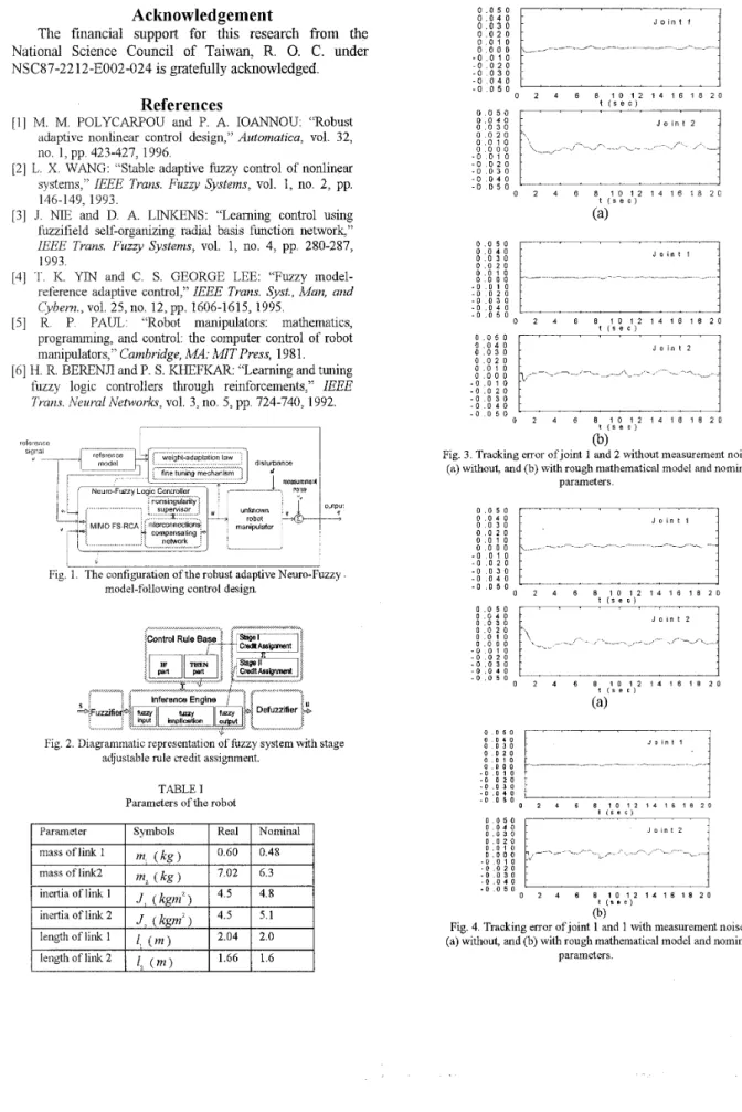
results are presented in Fig. 3. Fig. 3(a) and (b) show the case of the NFLC with and without using nominal parameters of the manipulator. We see from Fig. 3 that the NFLC achieves faster convergence when the initial parameters are chosen on the basis of nominal robot parameters.

Tracking control with measurement noise

The noise sources are assumed to be white with uniform distribution [-0.056, 0.051. We assume that the noise effects of different sensors are independent of each other. The external disturbances are set like the above subsection. Fig. 4 shows the tracking error of joint 1 and joint 2. Tlvs simulation shows that the proposed control

scheme is robust against measurement noise.

6. Conclusion

A method of robust neuro-fuzzy model-following

control for multi-link robot manipulators has been

constructed. The NFLC is composed of

an

multi-

inpudmulti-output

fuzzy

system with adjustable rule

credit assignment and interconnections coinpensatmg network. The interconnections compensating network can decompose the robot dynamics into decoupled subsystems and the fuzzy part approximates the unknown non-linearity of the robot by leamng By using fine tuning mechmsm in the consequent memberslup functions, the NFLC based control system can achieve

some degree of robust properties The overall robust

adaptation scheme has been proved to be able to

guarantee the output tracking error to converge to a

dual set ultimately. Simulations of an example plant

have confirmed the robustness of the design to actuator

input noise and measurement noise. If the rough plant model and parameters of the robot are available, the NFLC can be trained in advance to achieve faster convergence of the weight adaptation and model

Acknowledgement

The financial support for this research from the

National Science Council of Taiwan, R. 0. C. under

NSC87-22 12-E002-024 is gratefully acknowledged.

mass of link 1 mass oflink2 inertia of link 1 inertia oflink2 lzngth of link 1 leiigth of link 2

References

[ l ] M. M. POLYCARF'OU and P. A. IOANNOU: "Robust adaptive nonlinear control design," Automatica, vol. 32, no. 1, pp. 423-427, 1996.

[2] L. X. WANG: "Stable adaptive fuzzy control of nonlinear systems," IEEE Trans. F u z v Systems, vol. 1, no. 2, pp.

146-149, 1993.

[31 J. NIE and D. A. LINKENS: "Learning control using fuzzifield self-organizing radial basis function network,"

IEEE Trans. Fuzzy Systems, vol. 1, no. 4, pp. 280-287, 1993.

[4] 'I. I<. YIN and C. S. GEORGE LEE: "Fuzzy model- reference adaptive control," IEEE Trans. Syst., Man, and Cybem., vol. 25,no. 12, pp. 1606-1615, 1995.

[ 5 ] R. P. PAUL: "Robot manipulators: mathematics, programming, and control: the computer control of robot manipulators," Cambridge,

A&!:

MIT Press, 1981. [6] H. R. BERENJI and P. S. KHEFKAR: "Learning and tuning

fuzzy logic controllers through reinforcements," IEEE

Tvans. Neural Networlcs, vol. 3, no. 5 , pp. 724-740, 1992.

m, ( k g ) 0.60 0.48 m2 ( k g ) 7.02 6.3 J , (kgm') 4.5 4.8 J m z ) 4.5 5.1 1) ( 2.04 2.0 1.66 1.6 1, ( m ) 0"tP"t

1

network

2

model-following control design

Fig 1 The configuration of the robust adaptive Neuro-Fuzzy

. . . ... .

Fig. 2. Diagrammatic representation of hzzy system with stage adjustable rule credit assignment.

TABLE I

Parameters ofthe robot

Parameter

I

Symbols

I

Real

I

Nominal

I

J o i n t 1 - 0 0 1 0 - 0 0 2 0 - 0 0 3 0 - 0 0 4 0 - 0 0 5 0 0 2 4 6 8 1 0 1 2 1 4 1 6 1 8 2 0

:i;cii

- 0 . o 4 0

1

, , , , , , , ,

1

0 2 4 6 8 1 0 1 2 1 4 1 6 1 8 2 0 - 0 . o 5 0 1 ( s e c ) 0 0 5 0 0 . 0 4 0 0 . o 3 0 0 0 2 0 0 . 0 1 0 0 0 0 0 - 0 0 1 0 - 0 . o 2 0 - 0 0 3 0 - 0 0 5 0 - 0 . 0 4 0

1

, , , , , , j 0 2 4 6 8 1 0 1 2 1 4 1 6 1 8 2 0 1 ( s e c )

(a>

0 . 0 5 0 0 . o 4 0 0 . 0 3 0 0 . 0 2 0 0 . 0 1 0 0 . 0 0 0 - 0 . o 1 0 - 0 . o 2 0 - 0 . o 3 0 - 0 . o 4 0 - 0 . o 5 0 0 . o 5 0 0 0 4 0 0 . 0 3 0 0 . o 2 0 0 . 0 1 0 0 . o 0 0 - 0 . o 1 0 - 0 . o 2 0 - 0 0 3 0 - 0 0 4 0 - 0 0 5 0

i " ' " ' ' ' ' i

J o i n t 1 0 2 4 6 8 1 0 1 2 1 4 1 6 1 8 2 0 t ( s e c )

t " " " " ' l

J o i n t 2 0 2 4 6 8 1 0 1 2 1 4 1 6 1 8 2 0 t ( s e c )

CO>

Fig. 3. Tracking error ofjoint 1 and 2 without measurement noise, (a) without, and (b) with rough mathematical model and nominal

parameters. 0 . 0 5 0 0 . 0 4 0 0 . 0 2 0 0 . 0 1 0 - 0 0 1 0 - 0 . o 2 0 - 0 . o 3 0 - 0 0 4 0 - 0 . o 5 0 0 2 4 6 8 1 0 1 2 1 4 1 6 1 8 2 0 1 ( 5 e C ) 0 . o 5 0 0 . o 3 0 0 . o 2 0 0 0 1 0 - 0 0 1 0 - 0 0 2 0 - 0 . o 3 0 - 0 . 0 4 0 - 0 . o 5 0 J o i n t 2 ._/.- - ,,/- -,-I.. ... 0 . o 0 0 - - - 0 2 4 6 8 1 0 1 2 1 4 1 6 1 8 2 0 I ( s e c ) (a> 0 0 5 0 0 0 4 0 0 0 3 0 J o i n t 1 - 0 . o 3 0 - 0 . o 4 0 - 0 0 5 0 0 2 4 6 8 1 0 1 2 1 4 1 6 1 8 2 0 I ( r e C ) 0 . 0 4 0 J o i n 1 2 0 . 0 3 0 0 . 0 2 0 - 0 .o 1 0 - 0 .o 2 0 - 0 . 0 3 0 - 0 .o 4 0 - 0 .o 5 0 0 2 4 6 8 1 0 1 2 1 4 1 6 1 8 2 0 t ( s e c ) (b)

Fig. 4. Tracking error ofjoint 1 and 1 with measurement noise,

(a) without, and (b) with rough mathematical model and nominal