Pergamon 0305-0548(94)00036-0 Printed in Great Britain. All rights reserved
0305-0548/95 $9.50+0.00
A L G O R I T H M S F O R T H E C H I N E S E P O S T M A N P R O B L E M O N M I X E D N E T W O R K S
W e n Lea P e a r n t i " a n d C. M. Liu2:~
1Department of Industrial Engineering & Management, National Chiao Tung University, Hsinchu, Taiwan, R.O.C. and 2Kaohsiung Military School, Kaohsiung, Taiwan, R.O.C.
(Received August 1993; in revised form May 1994)
Scope and Purpose---Given an undirected street network, the celebrated Chinese postman problem (CPP) is that of finding a shortest postman tour covering all the edges (streets) in the network. The Chinese postman problem on mixed networks (MCPP), is an extension of the CPP, in which some streets from the network are allowed to be traversed in both directions, and others may be traversed in one specified direction only. Applications of the MCPP include: routing of newspaper or mail delivery vehicles, parking meter coin collection or household refuse collection vehicles, street sweepers, snow plows, and school buses; spraying roads with salt, inspection of electric power lines, or oil or gas pipelines, and reading electric meters. The M C P P has been shown to be NP-complete, and heuristic solution procedures have been proposed to solve the problem approximately. The purpose of this paper is to review the existing solution procedures, and present two modifications of the existing methods to obtain better problem solutions.
Abstract--The Chinese postman problem on mixed networks (MCPP), is a practical generalization of the classical Chinese postman problem (CPP), which has many real-world applications. The MCPP has been shown to be NP-complete. Therefore, it is difficult to solve the problem exactly. For this reason, heuristic solution procedures have been proposed to solve the problem approximately. In this paper, we first review two existing solution procedures proposed by Edmonds and Johnson [Math. Progr. 5, 88-124 (1973)], and Frederickson [J. Assoc. Comput. Mach. 26, 538-554 (1979)], then introduce two new algorithms to solve the M C P P near optimally. The proposed new algorithms are tested and compared with the existing solution procedures. Computational results showed that the two new algorithms significantly outperformed the existing solution procedures.
1. I N T R O D U C T I O N
The Chinese postman problem on mixed networks (MCPP), is an interesting generalization of the classical Chinese postman problem (CPP), in which the underlying (street) network is
mixed.
On mixed networks, some streets (edges) are allowed to be traversed in both directions (two-way) with equal distance, and others (arcs) may be traversed in one specified direction only (one-way). Such a generalization, of course, reflects real-life situations more directly. In particular, for cities with narrow streets, or where there is a need for traffic flow control.The M C P P may be briefly defined as follows. We are given a street network
G=(V, E, A)
with V representing a set of nodes, E representing a set of undirected edges (two-way streets), and A representing a set of directed arcs (one-way streets). For each edge (i, j) E E, we have two non-negative distances:d(i, j)
for the direction from node i to node j, and d(j,/) for the direction from node j to node i withd(j, i)=d(i, j).
For each arc (i, j)~ A, we have a non-negative distanced(i, j)
for the direction from node i to node j, and d(j, i) is set to infinity in this case. Then, the MCPP is to find a postman tour, starting from the depot, traversing each edge and arc in E u A at least once, andi'Dr W. L. Pearn received his Ph.D. degree from the University of Maryland at College Park, Maryland. His area of interest include network optimization, and quality management. He has been with AT&T Bell Laboratories, and currently he is a professor of Operations Research in the Department of Industrial Engineering and Management at National Chiao Tung University, Taiwan, R.O.C.
++Mr C. M. Liu received his M.S. degree from the Department of Industrial Engineering and Management, National Chiao Tung University. Currently, he is an instructor at Kaohsiung Military School, R.O.C.
480 Wen Lea Pearn and C.M. Liu
returning to the same depot with total distance traversed minimized. Clearly, if A = ~ , then the M C P P reduces to the classical CPP.
The solution to the C P P (defined on undirected networks) may be obtained efficiently using a polynomial-time bounded matching algorithm owing to Edmonds and Johnson [1-1. But, the M C P P (defined on mixed networks) has been shown to be NP-complete [2]. Christofides et al. [3"1 presented an integer programming formulation of the problem, and developed an exact algorithm to solve the M C P P optimally. The algorithm is essentially based on a branch-and-bound algorithm using Lagrangean relaxations. Minieka [4] presented a transformation converting the M C P P into a flow with gains problem, which allows the M C P P to be solved optimally via linear programming and cutting plane techniques. Unfortunately, b o t h approaches are computationally inefficient; only problems of small or moderate size may be solved optimally. Because of the problem's complexity, several heuristic solution procedures have been proposed to solve the M C P P approximately [1, 3, 5, 6]. In this paper, we first review the existing solution procedures, then present two new algorithms to solve the problem approximately.
2. REVIEW OF EXISTING SOLUTION PROCEDURES
Real-world applications directly related to the M C P P include: routing of newspaper [7] or mail delivery vehicles [8], parking meter or household refuse collection vehicles [9], street sweepers, snow plows and school buses [10]; spraying roads with salt [11, 121, inspection of electric power lines, or oil or gas pipelines, and reading electric meters [13].
An undirected network is called even if every node in the network has even degree. A directed network is called symmetric if for every node, i, in the network, deg ÷ (i)= deg-(i), where deg ÷ (i)= the number of arcs directed out of node i, and d e g - ( i ) = t h e number of arcs directed into node i. If the network is even (or symmetric), then a postman route can be constructed from the network without repeating any edges (or arcs). Details of this tour construction procedure may be found in Ref. [ 14].
Edmonds and Johnson [1"1 presented an algorithm to solve the M C P P approximately. The algorithm essentially consists of two phases. Phase I converts the original network into an even one by treating each (directed) arc as an (undirected) edge. Phase II transforms the network (obtained from the first phase) into a symmetric one. Since the transformed symmetric network is not necessarily maintained even, the postman tour may not be constructed. Frederickson [5] modified the algorithm by adding a new phase (Phase III). The new phase recovers the resulting network back to even so that a postman tour can be constructed. This algorithm was referred to as MIXED1. Frederickson [5] further considered an alternative approach, which is essentially the reverse of the Edmonds and Johnson [1] approach. The reverse approach first makes the network symmetric, then even. The reverse approach has been referred to as MIXED2. Other solution procedures such as those developed by Brucker [6-1, and Christofides et al. [3-1 are essentially the same as MIXED1 and MIXED2 and, therefore, will not be discussed here.
2.1. M I X E D 1 algorithm
Phase I. convert G into an even network.
Step 1. Let G* be the new network obtained from G with all arc directions ignored.
Step 2. Solve the C P P over the new network G* using the matching algorithm owing to Edmonds and Johnson [1]. Let Z(E) be the set of edges, and Z(A) the set of arcs obtained from the matching. We also let El = E w Z( E), A ~ = A u Z( A ). Then, G1 =(1I, E 1, A1) is even.
Phase II. transform G1 into a symmetric network.
Step 1. Construct a new network G 2 =(1 ,I, A2) with arc costs, arc capacities, and node
demands defined as: ,.
for each edge (i, j)~ El, create tbttrlnew arcs in .4 2 including (a) one copy of (i, j) with cost d(i, ) ) a n d infinite flow capacity, (b) one copy of (j, i) with cost d(i, j) and infinite flow capacity,
Step 2.
Step 3.
(c) one copy of (i, j), denote it as
(i, j)',
with cost zero and flow capacity 1, (d) one copy of (j, 0, denote it as (j, i)', with cost zero and flow capacity 1; for each arc (k,/)6A1, create one copy of (k,/) in A2, with costd(k, l)
and infinite flow capacity.for each node i6 V, define
(a) demand = {deg+(/) in G2} - {deg-(0 in Gz} ifdeg +(i) in G2 > deg-(/) in G2, (b) supply={deg-(/) in G2}-{deg+(0 in G2} if G2>deg+(/) in G2, where
deg+(/) = the number of arcs incident out of node i, and d e g - ( i ) = t h e number of arcs incident into node i.
Find the minimum-cost flow over the network G2. Let Yo, Y~, Yij,, Yjr, and Y~t be the number of flow units among the arcs (i, j), (j, i), (i, j)', (j,/)', and (k,/), respectively.
Construct a symmetric network G 3 =(V, E3, A3). Initially, we set E 3 = 0 , and
A 3 = A 1.
(a) if Y~j, + Yjr = 1, put
Yii"
copies of arc (i, j) andY~r
copies of arc (j,/) in A 3, (b) if Y~i' + Yjr # 1, put one copy of edge (i, j) in E3,(c) put Y~j copies of arc (i, j) and Yji copies of arc (j,/) in A 3, (d) put Ykl copies of arc (k, l) in A 3.
Phase IlL Recover G 3 back to even 15].
Let A' be the set of artificial arcs generated from Phase II, and
E4=E3.
Identify cycles from A' u E4 consisting of alternating paths in A' and E4, with each path anchored at each end by an odd node from G 3. In finding such cycles, directions of the arcs on paths from A' should be ignored. As the cycles cover all odd nodes from G3, directions will be arbitrarily assigned to the cycles, and arcs on the cycles will be either duplicated or deleted depending upon if the direction of the cycle is the same as the original direction of the arcs in A', and edges will be oriented. Consequently, all the nodes from G3 will be even and symmetric (for further descriptions, see Frederickson 1,5]). Denote the resulting network as G4.Phase I of the algorithm applies the minimum-cost matching algorithm to convert the original network into an even one. Phase II of the algorithm applies the minimum-cost flow algorithm to transform the resulting network into a symmetric one. And Phase III of the algorithm recovers the resulting symmetric network back to even. Frederickson [5] showed that the computational complexity of the algorithm is O(max{I VI a, Ial (max{IAI, IEI})2)}, where once again I VI--the number of nodes, iAI = the number of arcs, and IEI = the number of edges from the network. Frederickson I-5] further showed that the performance of this algorithm, in the worst case, has a bound of 2, that is, (MIXED1 Solution)/(Optimal Solution)~<2, and the bound is approachable.
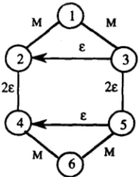
Example 1.
Consider the network depicted in Fig. 1 with six nodes, six edges, and two arcs. TheM M
2E
482 Wen Lea Pearn and C. M. Liu
associated edge and arc lengths are defined as follows: for edges, d(1, 2) = d(l, 3) = d(4, 6) = d(5, 6) = M, d(2, 4) = d(3, 5) = 2~; for arcs, d(3, 2) = d(5, 4) = ~, where M > e > 0. It is easy to verify that the solution obtained by MIXED1 contains artificial edges and arcs {(1, 3), (1, 3), (2, 1), (2, 1), (3, 2), (5, 4)}, and has a total length of 8M + 8~, while the optimal solution has a total length of 4M + 10s. Thus, we have (MIXED1 Solution)/(Optimal Solution) = (8M + 8~)/(4M + 10s)--. 2, as M >> e.
2.2. MIXED2 algorithm
Phase I. Transform G into a Step 1.
Step 2.
Step 3.
Construct a new demand defined for each edge (i, (a) one copy of (b) one copy of (c) one copy of (d) one copy of
symmetric network.
network Gt =(V, At) with arc costs, arc capacities, and node as:
j) e E, create four new arcs in At including (i, j) with cost
d(i, j)
and infinite flow capacity, (J, 0 with costd(i, j)
and infinite flow capacity,(i, j), denote it as
(i, j)',
with cost zero and flow capacity I, (j, i), denote it as (j, i)', with cost zero and flow capacity 1; for each arc (k,/)e A, create one copy of (k,/) in A1, with costd(k, l)
and infinite flow capacity.for each node i ~ V, define
(a) d e m a n d = {deg÷(i)in G~} - {deg-(i)in Gt} ifdeg÷(i)in G 1 > deg-(i)in GI, (b) supply={deg-(i) in G~}-{deg+(i) in GI} if deg-(i) in G t >deg+(i) in
G1, where deg÷(i)=the number of arcs incident out of node i, and deg-(i)= the number of arcs incident into node i.
Find the minimum-cost flow over the network Gt. Let
Yo, Yji, Y~j', Yji',
andYk~
be the number of flow units among the arcs (i, j), (j, i), (i, j)', (j, i)', and (k,/), respectively.Construct a symmetric network G2 = (V, E2, A2). Initially, we set E2 = ~ , and
A2=A.
(a) if
Yi~'
+ Yi~' = 1, put Y~j, copies of arc (i, j) andYj~,
copies of arc (j, i) in A2, (b) if Yo' + YJ~' ~ 1, put one copy of edge (i, j) in E2,(c) put Yii copies of arc
(i,j)
andYji
copies of arc (j, i) in A2, (d) putYkl
copies of arc (k, l) in A2.Phase IL Convert G 2 into an Eulerian network.
Step 1. Solve the C P P over the subnetwork of G consisting of E 2 and the associated
nodes using the matching algorithm of Edmonds and Johnson [1"1.
Step 2. Let Z(E2) be the set of edges obtained from the matching, and E 3 = E 2 u Z(E2),
A3 = A2. The Eulerian network G 3 =(V, E3, A3) is the desired solution.
Clearly, the computational complexity of MIXED2 is the same as that of MIXED1, i.e. O(max{I VI 3,
Ia{I
(maxlAI, IEI})2}). The bound on the worst-case performance of MIXED2 is also the same as that for MIXED1, and the bound is approachable.Example 2.
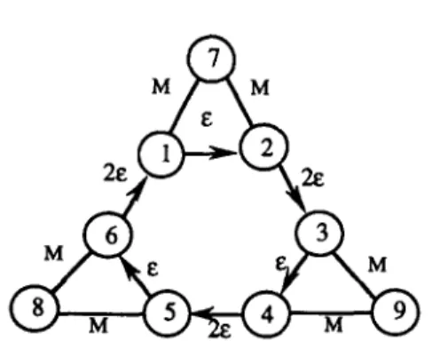
Consider the network depicted in Fig. 2 with eight nodes, six edges, and six arcs. The associated edge and arc lengths are defined as follows: for edges, d(1, 9) = d(2, 9) = d(3, 8) = d(5, 8) = d(4, 9) = d(6, 9) = M; for arcs, d(1, 2) = d(3, 4) = d(5, 6) = e, d(2, 3) = d(4, 5) = d(6, 1) = 2e, where M > e > 0. Clearly, the network is symmetric. Therefore, we may proceed with Phase II of the algorithm directly. It is easy to verify that the following artificial edges {(1, 7), (7, 2), (3, 9), (9, 4), (5, 8), (8, 6)} may be generated and the MIXED2 solution is 12M + 9e, while the optimal solution is 6M + 12e. Hence, we have (MIXED2 Solution)/(Optimal Solution) = (12M + 9e)/(6M + 12e) ~ 2, as M >> e.To improve the solution, Frederickson [51 considered a mixed-strategy approach. The mixed-strategy approach first calls MIXED1 and MIXED2 algorithms to generate two complete M C P P solutions, then selects the best of the two. We refer to this approach as MIXED1-2.
Fig. 2. The MCPP network described in Example 2.
Frederickson [5] showed that the worst-case bound for this approach, is 5/3. In fact, if we apply MIXED1-2 algorithm to example 1, then a solution of minimum {8M +8e, 4 M + 10e} = 4 M + 105 may be obtained, which is optimal. Similarly, if we apply MIXED1-2 algorithm to example 2, then a solution of minimum {6M + 125, 12M + 95} = 6M + 125 may be obtained, which is also optimal. 2.3. A comparison
To compare MIXED1 and MIXED2 algorithms. We generated 60 problems. Some of the test problems are dense networks, and others are sparse. These problems were generated by arbitrarily linking pairs of nodes so that a connected network is formed. The lengths of edges and arcs were also arbitrarily generated. These problems are described in the following with IV] representing the number of nodes, IEI representing the number of edges, [A] representing the number of arcs, and P representing the ratio tAI/(IAI + IEI) in the original M C P P network.
Set A: 5 problems; II/[=10; 2~<IEI~<5, 13~<1Al~<25, 70%<P~<100%. Set B: 5 problems; lVI--20; 2 ~ I E I ~ 19, 45~<lAl ~< 113, 70% <P~< 100%. Set C: 5 problems; IVI=30; 10~<lEl~<55, 115~<1Ar~<235, 70%<P~<100%. Set D: 5 problems; 1V1--35; 7~<1E1~<53, 238~<1A[~<302, 70%<P~<100%. Set A': 5 problems; IVl= 10; 7~<[Et~< 16, 10~<[a[~< 12, 40% <P~<70%. Set B': 5 problems; [V[=20; 28~<1E[~<61, 40~<1A1~<54, 40%<P~<70%. Set C': 5 problems; I VI = 30; 74 ~< IEI ~ 165, 86 ~< Ial -< 191, 40% < P ~< 70%. Set D': 5 problems; rvI = 35; 88 ~< lE[ ~< 186, 120~< [AI ~<274, 40% < P~<70%. Set A": 5 problems; [V[=10; 10 ~< [E[ ~<18, 3~<1A1~<5, 0 % < P ~ 4 0 % . Set B": 5 problems; I VI = 20; 55 ~< IEI ~< 101, 5 ~< IAI ~< 34, 0% < P ~< 40%. Set C": 5 problems; [V[=30; 108~<1E1~<216, 33~<1A1~<72, 0%<P~<40%. Set D": 5 problems; I VI = 35; 182 ~< [El ~< 266, 44 ~< [A[ ~< 131, 0% < P ~< 40%.
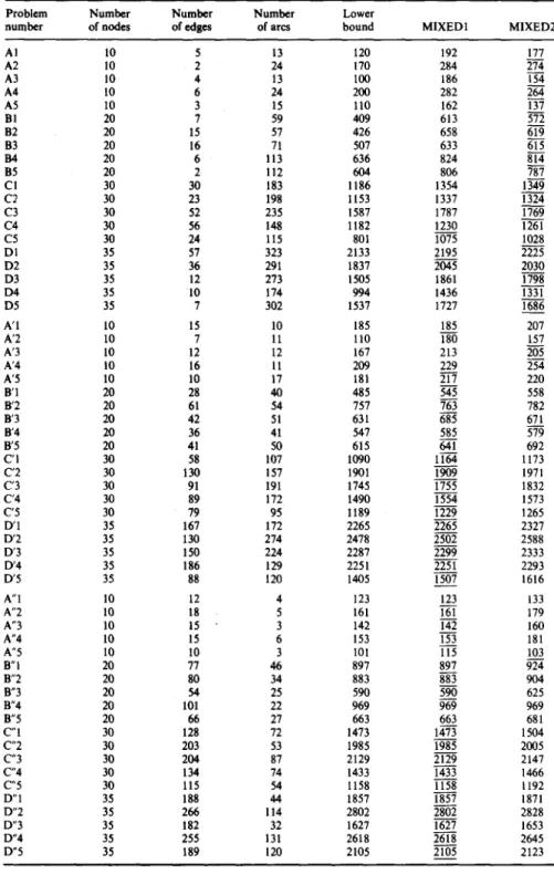
Table 1 presents the solutions generated by MIXED1 and MIXED2 on the 60 test problems. The lower bounds were obtained by solving the CPP over the (undirected) network derived from the original one by ignoring all the arc directions, which is to be used as a convenient reference point for assessing the accuracy of the heuristic solutions. In Table 2, the performance of MIXED1 and MIXED2 are compared. The results indicated that: (1) MIXED1 significantly outperformed MIXED2 for problems with 0% < P~< 70%, as MIXED1 received 33 best solutions out of 40 test problems (which is 82.5%), (2) MIXED2 significantly outperformed MIXED1 for problems with 70% <P~< 100% (most streets are one-way), as MIXED2 received 18 best solutions out of 20 test problems (which is 90%), and (3) MIXED1 performed extremely well on problems with 0% < P,<40% (most streets are two-way), as the algorithm received 19 problem optimal solutions out of 20 test problems (which is 95%).
3. NEW A L G O R I T H M S
Recall that MIXED1 first applies minimal-cost matching then minimum-cost flow algorithms. Both procedures generate artificial arcs. In some cases, these artificial arcs have the same direction
484 Wen Lea Pearn and C. M. Liu
Table !. Solution of the 60 test problems (underlines indicate the best solutions)
Problem N u m b e r N u m b e r Number Lower
number of nodes of edges of ares bound MIXED1 MIXED2
AI 10 5 13 120 192 177 A2 l0 2 24 170 284 274 A3 l0 4 13 100 186 154 A4 10 6 24 200 282 264 A5 10 3 15 110 162 137 Bl 20 7 59 409 613 572 B2 20 15 57 426 658 619 B3 20 16 71 507 633 615 I]4 20 6 113 636 824 814 B5 20 2 112 604 806 787 CI 30 30 183 1186 1354 1349 C2 30 23 198 1153 1337 1324 C3 30 52 235 1587 1787 1769 C4 30 56 148 1182 1230 1261 C5 30 24 115 801 1075 1028 DI 35 57 323 2133 2195 2225 D2 35 36 291 1837 2045 2030 D3 35 12 273 1505 1861 1798 D4 35 10 174 994 1436 1331 D5 35 7 302 1537 1727 1686 A'I 10 15 10 185 185 207 A'2 10 7 11 110 180 157 A'3 10 12 12 167 213 205 A'4 10 16 11 209 229 254 A'5 10 10 17 181 217 220 B'I 20 28 40 485 545 558 B'2 20 61 54 757 763 782 B'3 20 42 51 631 685 671 B'4 20 36 41 547 585 579 B'5 20 41 50 615 641 692 C'I 30 58 107 1090 1164 1173 C'2 30 130 157 1901 1909 1971 C'3 30 91 191 1745 1755 1832 C'4 30 89 172 1490 1554 1573 C'5 30 79 95 1189 1229 1265 D'I 35 167 172 2265 2265 2327 D'2 35 130 274 2478 2502 2588 D'3 35 150 224 2287 2299 2333 D'4 35 186 129 2251 2251 2293 D'5 35 88 120 1405 1507 1616 A"I 10 12 4 123 123 133 A"2 10 18 5 161 161 179 A"3 10 15 3 142 142 160 A"4 10 15 6 153 153 181 A"5 10 10 3 101 115 103 B"l 20 77 46 897 897 924 B"2 20 80 34 883 883 904 B"3 20 54 25 590 590 625 B"4 20 101 22 969 969 969 B"5 20 66 27 663 663 681 C"I 30 128 72 1473 1473 1504 C"2 30 203 53 1985 1985 2005 C"3 30 204 87 2129 2129 2147 C"4 30 134 74 1433 1433 1466 C"5 30 115 54 1158 1158 1192 D"I 35 188 44 1857 1857 1871 D"2 35 266 114 2802 2802 2828 D"3 35 182 32 1627 1627 1653 D"4 35 255 131 2618 2618 2645 D"5 35 189 120 2105 2105 2123
Table 2. Performance comparisons between M1XEDI and MIXED2 (60 problems)
Problem Algorithm N u m b e r Algorithm
Problem sets characteristics MIXED1 of ties MIXED2
A, B, C, D 7 0 % < P ~ I00% 2 0 18
A', B', C', D' 40% < P ~ 7 0 % 17 0 3
and therefore form cycles. From previous experiments we found that this situation occurs, particularly, when P = IAI/(IAI + IEI) is large. Obviously, such artificial cycles may be removed and solutions can be improved. This motivates the following modifications.
3.1. Modified MIXED1 algorithm Phase I. Same as MIXED1. Phase II. Same as MIXED1. Phase III. Same as MIXED1.
Phase IV. Remove artificial cycles from G4.
Let A* be the set of artificial arcs generated from Phases I, II, and III. Arbitrarily select an arc (i, j) from A*. Find a cycle (or a closed circuit) consisting of arcs from A* covering (i, j). Update A* by removing the cycle (circuit) from A*. Repeat this procedure until no more cycles (or closed circuits) can be found.
Finding artificial cycles (or closed circuits) covering a specified arc requires a shortest-path algorithm which is of O(I VI 2) (see Christofides I-15] and Pearn I-16] for such procedures). Therefore, the complexity of Modified MIXED1 is the same as that of MIXED1. For the M C P P with six nodes, six edges, and two arcs described in Example 1, the Modified MIXED1 algorithm removes the following artificial cycle {(1, 3), (3, 2), (2, 1)} generating a solution of 6M + 7e. Comparing this solution with that of MIXED1 which has a total length of 8M + 8e, the improvement is significant (particularly, when M >> e).
3.2. Modified MIXED2 algorithm
Recalling that in Phase II of MIXED2 algorithm the minimal-cost matching algorithm was applied over the subnetwork containing edges only. If the lengths of the edges are relatively large, MIXED2 may perform poorly. In attempting to improve the solution, we took an alternative approach by first duplicating some arcs, and assigning directions to edges to convert the network into an Eulerian one.
Phase I. Same as MIXED2.
Phase II. Convert G 2 into an Eulerian network.
Step 1. Solve the C P P over the subnetwork consisting of E 2 and the associated nodes using the matching algorithm of Edmonds and Johnson [1]. The shortest distance between each pair of nodes, however, was calculated from the original (mixed) network with all arc directions ignored.
Step 2. For each pair of nodes i and j in the matching solution, the shortest path between i and j (may be directed in this case) is added to G 2. If the added path is directed, then clearly other edges in E 2 must be oriented to maintain the resulting network symmetric.
The complexity of the Modified MIXED2 algorithm is the same as that of MIXED2. Applying this modified algorithm over the M C P P described in Example 2, the optimal solution, with a total length of 6M + 12e, can be obtained. In applying the matching algorithm, all arc directions have been ignored. Consequently, the following artificial edges {(1, 2), (3, 4), (5, 6)} rather than {(1, 7), (7, 2), (3, 9), (9, 4), (5, 8), (8, 6)} were generated resulting in a cost reduction of 6M-3e. Following the same idea described in Frederickson [5], we can also consider a mixed-strategy approach. That is, we first call Modified MIXED1, and Modified MIXED2, then select the best of the two solutions. We refer to this approach as Modified MIXED1-2.
4. C O M P U T A T I O N A L R E S U L T S
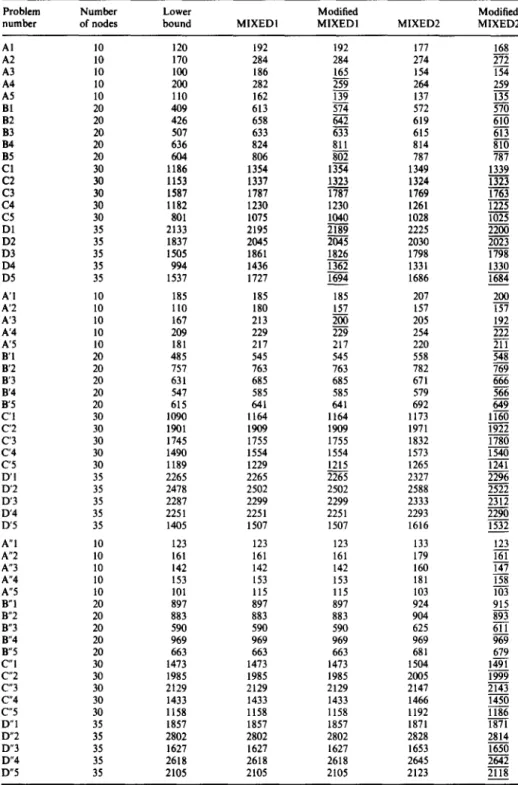
For the purpose of testing the proposed modifications arid comparing them with the original solution procedures, we ran the 60 test problems which have been tested in Section 2. Table 3 represents the solutions generated by the four algorithms, MIXED1; MIXED2, Modified MIXED1, and Modified MIXED2 on the 60 test problems with emphasizes indicating the improved solutions.
486 Wen Lea Pearn and C. M. Liu
Table 3. Solution of the 60 t a t problems (underlines indicate the solutions improved)
Problem Number Lower Modified Modified
number of nodes bound M1XEDI MIXED1 MIXED2 MIXED2
AI 10 120 192 192 177 168 A2 10 170 284 284 274 272 A3 10 100 186 165 154 154 A4 10 200 282 259 264 259 A5 10 110 162 139 137 135 Bl 20 409 613 574 572 570 B2 20 426 658 642 619 610 B3 20 507 633 633 615 613 B4 20 636 824 811 814 810 B5 20 604 806 802 787 787 C1 30 1186 1354 1354 1349 1339 C2 30 1153 1337 1323 1324 1323 C 3 30 1587 1787 1787 1769 1763 C 4 30 1182 1230 1230 1261 1225 C 5 30 801 1075 I040 1028 1025 D 1 35 2133 2195 2189 2225 2200 D 2 35 1837 2045 2045 2030 2023 D 3 35 1505 1861 1826 1798 1798 D 4 35 994 1436 1362 1331 1330 D 5 35 1537 1727 1694 1686 1684 A'I 10 185 185 185 207 200 A'2 10 110 180 157 157 157 A'3 10 167 213 200 205 192 A'4 l0 209 229 229 254 222 A'5 lO 181 217 217 220 211 B'l 20 485 545 545 558 548 B'2 20 757 763 763 782 769 B'3 20 631 685 685 671 666 B'4 20 547 585 585 579 566 B'5 20 615 641 641 692 649
C'l 30 I090 1164 I164 I173 If60
C'2 30 1901 1909 1909 1971 1922 C'3 30 1745 1755 1755 1832 1780 C'4 30 1490 1554 1554 1573 1540 C'5 30 1189 1229 1215 1265 1241 D'l 35 2265 2265 2265 2327 2296 D'2 35 2478 2502 2502 2588 2522 D'3 35 2287 2299 2299 2333 2312 D'4 35 2251 2251 2251 2293 2290 D'5 35 1405 1507 1507 1616 1532 A"I 10 123 123 123 133 123 A"2 I0 161 161 161 179 161 A"3 10 142 142 142 160 147 A"4 I0 153 153 153 181 158 A"5 10 101 I15 115 103 103 B"I 20 897 897 897 924 915 B"2 20 883 883 883 904 893 B"3 20 590 590 590 625 611 B"4 20 969 969 969 969 969 B"5 20 663 663 663 681 679 C"I 30 1473 1473 1473 1504 1491 C"2 30 1985 1985 1985 2005 1999 C"3 30 2t29 2129 2129 2147 2143 C"4 30 1433 1433 1433 1466 1450 C"5 30 1158 1158 1158 1192 1186 D"I 35 1857 1857 1857 1871 1871 D"2 35 2802 2802 2802 2828 2814 D"3 35 1627 1627 1627 1653 1650 D"4 35 2618 2618 2618 2645 2642 D"5 35 2105 2105 2105 2123 2118
Comparisons between modified MIXEDI and modified MIXED2
In Table 4, the performance of Modified MIXED1 and Modified MIXED2 are compared. The results obtained were quite similar to that for comparing MIXED1 and MIXED2:
(1) Modified MIXED1 significantly outperformed Modified MIXED2 for problems with 0% < P ~< 70%, as Modified MIXED1 received 28 best solutions out of 40 test problems (which is 70%);
(2) Modified MIXED2 significantly outperformed Modified MIXED1 for problems with 70% <P~< 100%, as Modified MIXED received 17 best solutions out of 20 test problems (which is 85%).
Table 4. Performance comparisons between Modified MIXEDI and Modified MIXED2 (70 problems)
Problem Modified Number Modified
Problem sets characteristics MIXED1 of ties MIXED2
A. B, C, D 70%<P<~100% 1 2 17
A', B', C', D' 40% <P~<70% 12 1 7
A", B", C", D" 0 % < P ~ < 4 0 % 16 3 1
Table 5. Percentage of problem solutions improved by the modifications (60 problems)
Problem Modified Modified Modified
Problem sets characteristics MIXEDI MIXED2 MIXED1-2
A, B, C, D 70%<P~<100% 65% 85% 85%
A'. B', C', D' 40% <P~<70% 15% 95% 40%
A", B", C", D" 0% <P~<40% 0% 85% 0%
Comparisons between modified approaches and the original algorithms
In Table 5, the performance between the proposed modifications and the original algorithms are compared in terms of the percentage of problem solutions improved. We note that:
(1) modified MIXED 1 improved MIXED 1 for 65 % of problems with 70% < P ~< 100%, 15% of problems with 40% < P ~< 70%, and no improvement for problems with 0% < P ~< 40% (we note that for 19 out of 20 problems in this category, MIXED1 obtained problem optimal solutions; therefore, very little improvement can be made);
(2) modified MIXED2 improved MIXED2 for 85% of problems with 70% < P~< 100%, 95% of problems with 40% < P-%< 70%, and 85% for problems with 0% < P ~< 40%. The improvement, clearly, is very significant.
For mixed strategies, Modified MIXED1-2 improved MIXED1-2 for 85% of the problems with 70% < P ~< 100%, 40% for problems with 40% < P,%< 70%, and no improvement for problems with 0% <P~<40%. We point out that this comparison is important since the two mixed strategies outperformed their corresponding MIXED1 and MIXED2 procedures. In Table 6, the performance of the four algorithms are compared in terms of average deviation from the lower bound, number of problems receiving the best solutions among all algorithms, number of problems achieving the problem lower bounds (in this case, the solution obtained is optimal), and the worst solution in terms of percentage above the lower bound. The results indicated that:
(1) for problems with 40%<P~<70% and 70%<P~<100%, Modified MIXED1 improved MIXED1 for about 1.5 and 4.4%, respectively;
(2) for problems with 0% < P ~< 40%, 40% < P ~< 70%, and 70% < P ~< 100%, Modified MIXED2 improved MIXED2 for about 2.6%, 3.4%, and 1.1%, respectively; (3) for problems with 0% < P ~< 40%, MIXED1 performed very well as the algorithm
received 19 problem optimal solutions out of 20 test problems (which is 95%). Consequently, no further improvements can be made by modified MIXED1; (4) for problems with large P (70% < P ~< 100%), none of the four algorithms seem
to work well (the average percentages above the lower bound for the four algorithms all exceed 25%). This is owing to the fact that our lower bounds were obtained from solving the CPP over the (undirected) network derived from the original one by ignoring all the arc directions.
In our testing, the run times for problems of the same size are very much the same. Therefore, instead of showing the average run time, we only display (Table 7) six test problems in CPU seconds on the IBM 486 as an indication of the relative efficiency of the four algorithms. We note that all the four algorithms are very efficient. A problem with 35 nodes, and 350 edges and arcs only takes less than 2 C P U seconds. It should be pointed out that the run times difference between the modified
488 Wen Lea Pearn and C. M. Liu
Table 6. Performance comparisons of the four algorithms (60 problems)
Problem Modified Modified
characteristics MIXEDI MIXED1 MIXED2 MIXED2
Average percentage above 70% < P ~< 100% 33.46 29.10 26.80 25.69
the lower bound 40% < P ~< 70% 8.89 7.39 10.89 7.5
0% < P ~< 40% 0.69 0.69 4.03 1.41
Number of problems 70% < P ~< 100% 0 3 4 19
receiving the best 40% < P ~< 70% 11 13 1 8
solution 0% < P ~< 40% 19 19 2 4
Number of problems 70% < P ~< 100% 0 0 0 0
achieving the lower 40% < P ~< 70% 3 3 0 0
bound 0% < P ~< 40% 19 19 1 3
Worst solution among 70% < P ~< 100% 86.00 67.06 61.18 60.00 60 problems in term of 40% < P ~< 70% 63.64 42.73 42.73 42.73
percentage above the 0% < P ~<40% 13.86 13.86 18.30 3.56
lower bound
Table 7. Run time comparisons (in CPU s) of the four algorithms
Problem Number Number Number Modified Modified
number of nodes of edges of arcs MIXED1 MIXED2 MIXED1 MIXED2
BI 20 7 59 0.110 0.055 0.110 0.055 B'I 20 28 40 0.110 0.165 0.110 0.165 B"I 20 77 46 0.165 0.165 0.165 0.165 C1 35 57 323 1.879 0.824 0.879 0.824 C' 1 35 167 172 1.154 1.099 1.154 1.099 C" 1 35 188 44 0.604 0.549 0.604 0.549
approaches and the original solution procedures for the same test problem, is negligible (less than 0.055 CPU seconds). Therefore, the difference does not show in Table 7.
5. C O N C L U S I O N S
In this paper, we presented two efficient modifications of the existing algorithms (MIXED1, MIXED2), which we referred to as Modified MIXED1 and Modified MIXED2. The two modified procedures run very fast, and work well in general. We have tested them on many problems which were arbitrarily generated. The computational results indicated that: (1) modified MIXED1 improved MIXED1 for 65% of problems with 70%<P~<100%, and 15% of problems with 40% <P~<70%, (2) Modified MIXED2 improved MIXED2 for 85% of problems with 70%<P~<100%, 95% of problems with 40%<P~<70%, and 85% of problems with 0% <P~<40%. For mixed strategies which are the procedures of choice, Modified MIXED1-2 improved MIXED1-2 for 85% of the problems with 70% < P~< 100%, and 40% of problems with 40% < P~< 70%.
R E F E R E N C E S
1. J. Edmonds and E. Johnson, Matching, Euler tours and the Chinese postman. Math. Progr. 5, 88-124 (1973). 2. C. H. Papadimitriou, O n the complexity of edge traversing. J. Assoc. Comput. Mach. 23, 544-554 (1976).
3. N. Christofides, E. Benavent, V. Campos, A. Corbran and E. Mota, An optimal method for the mixed postman problem.
Proceedings of the l l th IFIP Conference, Copenhagen, Denmark, pp. 641-649 (1983).
4. E. Minieka, The Chinese postman problem for mixed networks. Mgmnt Sci. 25, 643-648 (1979).
5. G.N.Fredericks•n•Appr•ximati•na•g•rithmsf•rs•mep•stmanpr•b•ems.J.Ass•c.C•mput.Mach.•6•538-554(•979).
6. P. Brucker, The Chinese postman problem for mixed graphs. Lecture Notes Comput. Sci. 100, 354-366 (1981). 7. L. Levy and L. Bodin, Scheduling in the postal carriers for the United States postal service: an application of arc
partitioning and routing. In Vehicle Routing: Methods and Studies, pp. 359-394. North-Holland, Amsterdam (1988). 8. J. N. Holt and A. M. Watts, Vehicle routing and scheduling in the newspaper industry. In Vehicle Routing: Methods
and Studies, pp. 347-358. North-Holland, Amsterdam (1988).
10. J. Desrosiers, J. A. Ferland, J. M. Rousseau, G. Lapalme and L. Chapleau, An overview of a school busing system. In
Scientific Management of Transport Systems, pp. 235-243. North-Holland, Amsterdam (1988).
11. R. W. Eglese and L. Y. O. Li, Efficient routeing for winter gritting. J. Opl Res. Soc. 43, 1031-1034 (1992). 12. R. W. Eglese, Routeing winter gritting vehicles, to appear in Discrete Appl. Math. (1992).
13. H. I. Stern and M. Dror, Routing electric meter readers. Comput. Ops Res. 6, 209-223 (1979). 14. A. Nijenhuis and H. S. Wilf, Combinatorial Algorithms. Academic Press, New York (1978). 15. N. Christofides, The optimal traversal of a graph. Omega 1, 719-732 (1973).