A boundary-element-based
optimization
technique for design
of enclosure
acoustical
treatments
T. C. Yang
Center for Measurement Standards, Industrial Technology Research Institute, 321 Sec. 2, Kuang Fu Road, Hsinchu 30042, Taiwan, Republic of China
C. H. Tseng
Department of Mechanical Engineering, National Chiao Tung University, 1001 Ta Hsueh Road, Hsinchu 30050, Taiwan, Republic of China
S. F. Ling
School of Mechanical and Production Engineering, Nanyang Technological University, Nanyang Avenue, Singapore 2263, Singapore
(Received 7 September 1994; revised 31 January 1995; accepted 16 February 1995)
An effective design tool was developed in this study for solving the acoustical treatments in enclosures at low frequencies. The boundary element method was used for accurately predicting sound fields of an acoustical system. The sequential quadratic programming was selected as the continuous design variable optimizer as a result of its robustness and rapid convergence. In coping with the noncontinuous design variables, the optimizer was enhanced by a modified branch and bound procedure. A small two-dimensional cavity and an irregularly shaped car cabin were applied to demonstrate the utilities of the proposed design tool. Computer simulations indicated that at a low frequency, where enclosures can properly be termed as tightly coupled, purely reactive acoustical
treatments
are
generally
preferred
at resonances
or near-resonances
of the
two-dimensional
cavity
as
well as at the frequency of interest in the car cabin. The general agreement between this study andprevious work [R. J. Bernhard and S. Takeo, J. Acoust. Soc. Am. 83, 2224-2232 (1988)] could be
considered adequate for the proposed tool to be utilized for preliminary design studies of acoustical treatments in enclosures. Furthermore, in the case of multiple patching, the optimal locations of acoustical treatments would always contain the region of dominantly acoustical influence. However, simultaneous capability of optimizing locations and impedances of acoustical material were not considered in the previous work. ¸ 1995 Acoustical Society of America.
PACS numbers: 43.50.Gf, 43.55.Ka, 43.55Dt
INTRODUCTION
The design of effective noise control treatments for en- closures where typical dimensions are comparable with acoustic wavelengths, and/or sound sources and enclosures are geometrically complex, is relatively difficult. Such acoustical cavity systems are complicated by the near-field source effects, standing wave characteristics, and low- frequency behavior of typical sound treatments. The passen- ger compartments of a car and a propeller-driven aircraft, and enclosures of close-fitting appliances and business ma- chine enclosures are such important applications where ei- ther the noise source is of low frequency or the enclosure is quite small. However, effective design procedures for such
applications
are rarely
due to the complexity
of the prob-
lems. Therefore, a reliable modeling procedure capable of accurately predicting the acoustical behaviors in enclosures as well as providing the design optimization information is fundamentally necessary.
Absorption of the low-frequency components of un- wanted noise in cavities is difficult and expensive by con- ventional methods of using porous materials because of the thickness required. Through the extensive investigations of
Maa
1'2 and Lee and Swenson,
3 however,
noise
control
for
low frequencies by passive techniques has become practical.
Thus the possibility of employing passive techniques to ef- fectively control low-frequency sound radiated from some- where inside the cavity appears worthy of investigation.
Previous studies on the modeling techniques were useful for enclosures where either high-frequency statistical behav- ior can be assumed or the geometrical configuration is rela-
tively
simple.
4-7 In this
study,
simulation
results
obtained
by
optimally placing acoustical materials on the boundary of enclosures are provided to achieve a better noise control. The boundary element method (BEM), emerging as a powerful alternative to the finite element method (FEM) and only dis- cretizing the surface rather than the volume, is chosen as an analysis tool for evaluating the acoustical characteristics in enclosed spaces. An optimizer employing the sequential qua-dratic
programming
(SQP)
algorithm
8 is integrated
with the
boundary element acoustical analysis for accurately solving the aforementioned acoustical treatment problems in cavities. Locating the proper positions of the sound absorbing materials on the boundary of enclosures is nearly impossible without the assistance of optimization techniques. In previ-ous
work,
e.g.,
Bernhard
and
Takeo,
7 only
the acoustical
im-
pedances of absorbing materials in a fixed position were op- timized; in addition, all of the design variables were considered as the continuous type. However, both the acous- 302 J. Acoust. Soc. Am. 98 (1), July 1995 0001-4966/95/98(1)/302/11/$6.00 ¸ 1995 Acoustical Society of America 302dd
,% ,©%
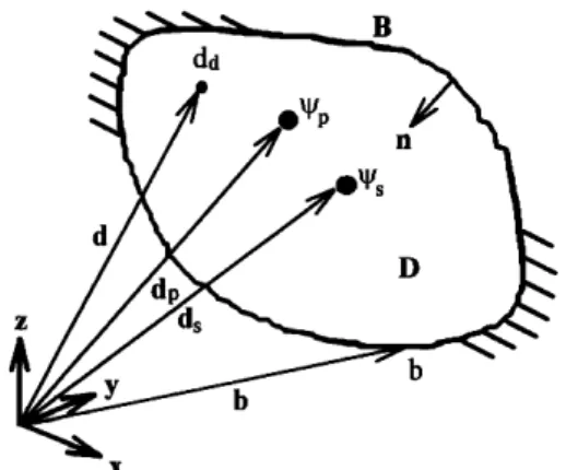
FIG. 1. Domain of acoustic system utilized for interior Helmholtz wave equation.
tical impedance and location of the absorbing material are simultaneously determined in this study for making the po- tential technique useful. Constraints, i.e., geometrical and/or functional, are also included as required due to practical con- siderations. From practical and economic concerns, only some boundaries of the cavity can be reserved for acoustical treatments. The acoustical material is not positioned any- where but is rather patched at specified regions during the optimization process. In coping with this difficulty, noncon- tinuous design variables capable of fully describing the pa- rameter of specified regions must therefore be introduced in addition to continuous ones. As a consequence of manipulat- ing the problems associated with continuous and noncontinu- ous design variables, the SQP scheme is enhanced by a
modified
branch
and
bound
method
(BBM)
9-11
to effectively
solve a general nonlinear passive noise control (PNC) opti- mization problem. Treating the PNC optimization in such a manner is the primary focus of this study, which is of essen- tial concern for design engineers but has not yet been con- sidered in a previous work.An optimization problem is formed in this study which optimizes allocations of acoustical materials on the boundary in cavities by minimizing the objective function which is subjected to suitable constraints. Total acoustic potential en- ergy of the control volume, similar to those in noise control problems, is selected here as the objective function. The op- timization is performed in the frequency domain by assum- ing that the noise source is of harmonic excitation. Next, computer simulations of acoustical treatments in enclosures are performed and discussed for different arrangements. In those simulations, a two-dimensional cavity is used to verify the BEM-based optimization design tool. An irregularly shaped car cabin is then modeled for further studies.
I. BOUNDARY ELEMENT FORMULATION IN
ACOUSTICS
Indirect
BEM as derived
by Chen
and
Schweikert
12
is a
numerical technique that can be used to calculate the sound fields in a three-dimensional space. The method is a numeri- cal implementation of Huygen's principle in acoustics. The optimal acoustical treatments on the boundary of the enclo- sures in this study are simulated from the response at field points of an acoustic system as illustrated in Fig. 1. Thus thederivation of optimal passive noise controllers can be formu- lated by using the indirect BEM technique. The numerical implementation of the indirect B EM technique in this study is customized from the general boundary element formula- tion. In summary, the process can be divided into the follow- ing steps.
Step 1: The nonhomogeneous Helmholtz equation,
V2p
+ k2p
= ½s(Xs),
is utilized
in forming
the
problem,
where
p is the complex acoustic pressure and k is the wave number. The point noise source of strength ½s is located at xs.Step 2: The general form of indirect BEM integral equa- tions for pressure, velocity, and impedance (locally reacting) boundary conditions, respectively, are written as
p(•)=
fBrr(b)p*(b,•)dB+
fz>½s(Xs)p*(Xs,•)dD,
(1)
U(•)=CbCr(•)+
fbCr(b)u*(b,•)dB
+ zOs(Xs)U*(Xs,e)dD,
(2)z(e)=p(e)/u(e), (3)
where o'(b) represents the fictitious source density function at the boundary point b, C b is an integration constant as a
result
of the
integral
singularity,
13
and
• is a dummy
variable.
The fundamental pressure solution p* is the free spaceGreen's
function,
p*(b,•)= 1/[b-•l e-je b-e and
the
fun-
damental
velocity
solution
u* can
be related
TM
to p* by Eu-
ler's equation, p 8u/Ot=-Vp, where p is the density of air.Step 3: A noncompatible, rectangular, linear element is selected to discretize the boundary of the acoustic system. Consequently, results can be obtained with reasonable com- puter capacity and time as a result of the need of optimiza- tion and model with a large number of elements. The volume
integrals of ½s in Eqs. (1), (2), and (3) are then replaced by
the summation term in light of the point noise sources. Hence, Eqs. (1), (2), and (3) are rewritten as
N e
P(bi)
=
j=lE fB
' Jø'(bj)p*(bj'bi)dBj
Nsq-
E •tsl(Xsl)p*(Xsl,bi),
/=1 (4) N eu(bi):Cbø'(bi)q-jE
ß =1
fB
jø'(bJ)u*(bj'bi)dBj
Nsq-
E •tsl(Xsl)lt*(Xsl,bi),
/=1 (5)0=
rr(bj)p*(bj
,bi)dBjn
t-
• ½sl(Xsl)P*(Xsl,bi)
j=l ' J /=1-z(bi)(CbO'(bi)-•-••BO'(bj)Ig*(bj,bi)dB
j=] Jj
)
-3-
• IPsl(Xsl)l•lV•(Xsl
,bi) ,
(6)
/=1where N e is the number of elements, Ns is the number of
noise
sources,
Bj is the boundary
contained
by the jth ele-
ment, and b i is the i th node.
Step 4: A system of N e equations for the N e unknown o-'s is obtained by writing Eqs. (4), (5), and/or (6) for each element according to the given boundary conditions. Thus a compact matrix form of Eq. (7) is solved for the fictitious source strength o- of each element:
Atr= a-bus, (7)
where matrices A and B are computed from Eqs. (4), (5), and/or (6), and vector a contains the values of boundary conditions. For instance, if element i has a pressure boundary condition, then
Aij-
fBjP*(bj,bi)dBj, (8)
Bil=P*(Xsl ,bi), (9)
o•i=p(bi). (10)
Step 5: Finally, Eqs. (4) and (5) are used to find the acoustic pressure and particle velocity of the interior points, in which the boundary point b i is replaced by the domain point xi.
II. MATHEMATICAL MODEL FOR OPTIMIZATION PROBLEM
Generally, three elements are included in a well-defined mathematical statement of the constrained design optimiza- tion, i.e., design variables, objective function, and design constraints. The primary objective of this study is to form an optimization problem capable of optimizing placements of acoustical materials on the boundary of a cavity. Each ele- ment of optimization is described in the following.
A. Design variables
Assuming that the acoustical materials is only locally reacting, the normal impedance has the form R(f )-jX(f ), where R and X are the resistance and reactance parts, respec-
tively,
and
are dependent
on frequency
f.]5 From
a practical
perspective, the candidates of design variables can be the number of pieces (n), centroid location (x,y,z), normal im- pedance (R,X), and size (A) of acoustical materials. The material-patched code (X) of a boundary element can also be a design variable, where X= 1 or 0 implies that the element does or does not cover the acoustical materials. For brevity sake, the size of the acoustic materials is selected as the area of the boundary element, i.e., the size A is a constant. If thecharacteristic of the noise source is known and the sound field is only controlled by the acoustical materials, the acous- tic pressure at field points of the cavity can be represented by
pi=Pi(n,x,y,z,R,X,X), i- 1,Nfp,
(11)
where
Nfp is the total number
of field points.
B. Objective function
Various objective functions have been used for the opti- mization of noise control, i.e., the total acoustic potential
energy
by Jo and
Elliott,
•6 weighted
sum
of the magnitudes
of the squared
pressures
by Mollo and
Bernhard,
17
average
of acoustic
pressures
ratio
by Tanaka
et al. 18
total
acoustic
power
by Cunefare
and Koopmann,
19 and space-average
sound
energy
density
by Yang
et al.
2ø
All of these
functions
are deemed effective as a performance index, even though a slight difference occurs among them. The total acoustic po- tential energy of the control volume is, however, selected as the objective function in this study. Two control strategies,
local
and
global,
2• can
be applied
where
necessary.
The ob-
jective function for various control strategies can always be formulated as'
(I)--
4pc2 Ip(n,x,y,z
g,x,x)l
2 dV,
(12)
where c and V are the speed of sound and the control vol- ume, respectively. The (I) can only be measured by ideal distributed sensors, which may not be practical for applica- tion purposes. In practice, a reasonable number of acoustical pickups are uniformly positioned in the cavity to accumulate the response for formulating the discrete form of the objec- tive function, as illustrated by Eq. (13)'
V Nfp
V-
2 • IPi(n,x,Y,z,R,X,K)I
2.
(13)
4pc i=i
This form is implemented in the numerical simulations. The control volume V can notably be taken out of the summation only if the acoustical pickups are uniformly distributed throughout the cavity. Otherwise, the contribution of each pickups must be weighted.
C. Design constraints
All engineering systems are designed to perform within a given set of constraints which include limitations on re- sources, material failure, response of the system, and mem- ber sizes. Three types of constraints are introduced in this study, i.e., design bounds, equality constraints, and inequality constraints. Possible candidates for each type are defined in the following. 1. Design bounds O•< n•< Ne , (14) x•<xi•<Xu, i=l,n, (15) y•<yi•<yu, i-l,n, (16) z•<zi•<zu, i= l,n, (17)
Rl•<Ri•<R u, i=l,n, (18)
Xi•<Xi•<Xu, i= 1,n, (19)
kj•{0,1},
j=l,Ne,
(20)
where the subcripts 1 and u represent the lower and upper bound of the design variables, respectively.
2. Equality constraints
Xi+X2+'" +XiVe=n.
(21)
This constraint implies that the sum of the patched codes must be equal to the number of pieces of acoustical materials utilized.
3. Inequality constraints
If the user wishes to maintain the specified sound pres-
sure level (SPL) at particular locations, e.g., conforming to
mandatory regulations, the following equation can be consid- ered:
SPL at (xj,yj,;zj)-Lp•<O, j= 1,Nsp
1,
(22)
where
Lp and Nsp
1 are the specified
SPL and number
of se-
lected locations, respectively.
D. Summary of optimization model
In summary, the design optimization model of this study finds the number of pieces (n), location (x,y,z), and imped- ance (R,X) of acoustical materials so as to minimize the total acoustic potential energy, which satisfies the required constraints. Generally, the aforementioned constrained opti- mization problem can be described mathematically while minimizing the objective function
f ( x) = f (x i ,x2 ... X2v), subject to the constraints
(23)
h i(x) = 0, i = 1 ,Neql,
(24)
gj(x) •< 0, j = 1 ,Niq•,
(25)
and the design bounds
x•<x•<Xu, (26)
where
Neq
1 and
Niq
1 are the number
of equality
and
inequality
constraints, respectively. It is a general mathematical model for the nonlinear single-objective constrained optimization problem. The optimum design x can be obtained by employ- ing efficient minimization algorithms capable of solving the related subproblem for determining the search direction, as well as determining the step size by minimizing the descent function. 8
E. Optimization algorithm
Multiple minima basically exist in the feasible domain of the preceding optimization problem along with a number of numerical nonlinear programming (NLP) methods which are capable of solving it. However, the sequential quadratic
programming (SQP) is selected in this study because of its
robustness
and
rapid
convergence.
22-24
The SQP
algorithm
is
a generalized gradient-descent optimization method and sub- sequently converges to a local rather than global optimum. This optimization method solves the quadratic programming subproblem to produce the direction of design improvement, and a step size along the search direction. The subproblem is obtained by using a quadratic approximation of the Lagrang- ian and linearizing the constraints as follows:
min •7f(xk)
r Axk+0.5 Ax•I-I
r Ax •,
subject to
and
hi(xk)
+ •7hi(xk)
r Axk=0,
g/(x•)
+ Vg/(x•)
r Ax•<0,
(27)
i= 1 ,Neql,
(28)
j= 1 ,Niql,
(29)
x•< x • + Axk•<
Xu,
(30)
where H is a positive definite approximation of the Hessian matrix, which is composed of the second partial derivatives of the Lagrangian function with respect to each of the design
variables,
and
x • is the
current
iterate.
The
Lagrang•an
func-
tion is formed here in terms of the objective function andconstraints and is defined as L(x,l•)=f(x)+•/•ihi(x )
+•/•jgj(x), where
/z is the Lagrange
multiplier.
If Ax
• is
selected as the solution of the subproblem, a line search can
be utilized
in finding
the new point
x • + •, i.e.,
x•+ •=xk + •7• Axe,
(31)
where
the step
size •7•
is selected
as 0.5
J with J as the small-
est positive integer which satisfies a descent function having
a lower value at the new point.
8 The descent
function
is
basically formed by the objective function and maximum
constraint
violation
8 due
to its simplicity
and
success
in solv-
ing a large
number
of engineering
design
problems.
25'26
This
iteration process is continued until the convergence test is passed; otherwise, the design variables are updated and the new iteration is executed.
To make use of well-established continuous optimiza- tion algorithms, most discrete optimization techniques are based on the assumption of transforming the noncontinuous solution space into multiple continuous solution sub-spaces. The optimization problems in each of these continuous sub- spaces are solved sequentially by imposing constraints on discreteness of the design variables. The optimal discrete so- lution is selected from among the continuous solutions ob- tained. The conventional discrete optimization techniques re- quire too many executions of the continuous optimization
scheme
and,
thus,
is very
time consuming.
9
Here,
an enhanced
branch
and
bound
method
(BBM)
•ø'•
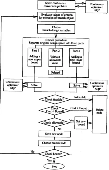
is employed to cope with the obstacles arising from noncon- tinuous design variables. In order to locate a discrete optimal solution using continuous optimization schemes, the BBM repeatedly delete portions of the original design space that do not contain allowable values of the noncontinuous design variables. This procedure is referred to as "branching." As illustrated in Fig. 2, the original design space is first divided into three sub-spaces with the allowable noncontinuous de- sign values nearest the continuous optimal solution as the upper and lower bound of the left and right sub-spaces, re-
Continuous
optimizer
SQP
• Sc
Solve continuous Continuous
conversion problem optimizer
[ SQP
•[ Evaluate values of criteria
-•for selection
of
branch
object
I
Choose
branch design variables Branch procedure:
Separate original design space into three parts
Pa[rtl
I [ Pa[rt2
] [ Paint3
Adding a ] [ Without [ } Ad•ng a
new upper I
.bound
[ lallowable
I value
] !new
bot
lower[
nd
optimizer SQP
Ch,,e;i•e..c•
C
ost
Infeasible
>
Bound
•[
• Delete
I
node{
]
I Choo
branch
I
No
,:.•:.(• ...
FIG. 2. Conceptual flow chart of the noncontinuous optimizer BBM.
spectively. The branching procedure must be repeated in each of the sub-spaces until a feasible optimal design is lo- cated. Each design sub-space is depicted as a "node" and a diagram of the branching is referred to as the "tree" of BBM. Theoretically, a discrete solution can be found if an exhaustive search of the tree is made.
If a feasible noncontinuous solution is obtained in the process of branching, the corresponding objective function value can be taken as a bound. Any other design sub-spaces that possess a continuous minimum cost larger than this bound need not be further branched since it would only gen- erate higher cost values. This strategy is referred to as "bounding" and can be used to select a branching route in- telligently, thereby avoiding complete and impartial search- ing through the tree.
Furthermore, all the procedures of the constrained opti- mization model defined in this study are incorporated into an architectural framework for the proposed design tool, as il- lustrated in Fig. 3. The communication between the BEM acoustical analysis and the BBM enhanced SQP optimization during the solution procedure is also shown in this architec- tural framework.
Input f'fle
INPUT
Read input data
BBM Non-continuous design variable treatment Optimization
Input
f'de
Sound field computation Objective Constraint SQP Single-objective continuous design variable optimizerBoundary element analysis
Output f'de
FIG. 3. Architectural framework of the proposed design tool, where cuserxx routines are user supplied functions. The cusermf and cusermg compute values of the objective and constraint functions, respectively. The cusercf and cusercg calculate gradients of the objective and constraint functions, respectively. However, the cuserou can provide additional data for verifica-
tion.
III. COMPUTER SIMULATIONS
A. Verification of the BEM-based optimization algorithm
Numerical characteristics of the developed BEM-based optimization technique are investigated by conducting a computer simulation for design of acoustical treatments in a two-dimensional cavity (Fig. 4). The cavity with two open- ings has a dimension of 0.56X0.32X0.08 m, i.e., slightly
different
from the one utilized
by Bernhard
and Takeo.
7 A
point
noise
source
of volume
velocity
1 m3/s
is positioned
at
(0.14, 0, 0.04) and is a harmonic source at frequencies rang- ing between 1500 and 2000 Hz.Two configurations of acoustical treatments, C1 and C2 (Fig. 4), are first simulated to make a qualitative comparison of the results with the concluding remarks in the previous
work,
7 i.e., (1) it would
appear
that
at a low frequency,
where
C1
Noise source
Openings
FIG. 4. Schematic diagram of a two-dimensional cavity utilized in Sec.
IIIA
• 600
•
•
1000
• 400 • soo • 200 o 0•
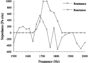
-200-500
x -1000 x -1500 -600 1500 1600 1700 1800 1900 2000 1500 1600 1700 1800 1900 2000 Frequency(I-Iz) Fre•ency (Hz)FIG. 7. Optimal acoustical •eatments versus •equency at C2 configuration. FIG. 5. Optimal acoustical •eatments versus •equency at C1 configurationß
enclosures can properly be termed as tightly coupled, purely reactive noise control treatments are preferred; (2) there is also a particular optimal reactive impedance depending on the frequency, geometry, and design objective function. For illustrative purposes, the impedance (R,X) of acoustical ma- terials is selected as the only design variable (i.e., acoustical material being fixed at specified location). The design bounds are set to 0•<R•<1000 Pa s/m and -2000<•X•<2000 Pa s/m. No physical constraints are involved in this case. Consequently, acoustical impedance at fixed configuration (i.e., n = 1) is optimized with the noise source of resonant or off-resonant excitation. Typical results are summarized in Figs. 5-8. The following general statements can be drawn from these numerical simulations.
(1) The optimal impedances of acoustical material vary with the exciting frequencies of the noise source and also change with locations of acoustical treatments. At resonances (i.e., 1540, 1610, and 1840 Hz in the frequency of interest) or near resonances, the optimal noise control treatments in this small cavity are more or less purely reactive (see Figs. 5 and 7) as a result of attenuation of the noise level by altering the mode shape. These remarks are quite similar to those
concluded
by Bernhard
and
Takeo.
7
(2) In light of no obvious mode shape, however, the mechanism of controlling the noise level at off-resonances of
the cavity can be different from that described at resonances. As also shown in Figs. 5 and 7, resistances (i.e., absorption) of the acoustical material are required in the off-resonant excitations for globally dissipating the acoustic energy in the control volume for better noise reduction.
(3) The objective function at resonances or near- resonances of the cavity decreases dramatically while the optimal impedances are obtained (Figs. 6 and 8). This can be considered as a consequence of a large reduction of SPL in the control volume. However, the objective function is insen- sitive to the variation of impedances of acoustical materials at off-resonances. Thus, the global minimum of this situation is difficult to be located. The local minimum can definitely be accepted from an engineering perspective if the improve- ment of design is obvious.
In summary, the major remarks of this simulation corre-
late sufficiently
with those
of Bernhard
and
Takeo.
7 Further
studies of acoustical treatments in enclosures are thus sup- ported by utilizing the proposed design tool of this work. Due to the powerfulness of the BBM enhanced SQP algo- rithm, the location and impedance of acoustical materials as design variables are simultaneously solved for the aforemen- tioned case. Two more configurations, C3 and C4, are added to the current case for further investigations (Fig. 9). Addi- tionally, design bounds of impedance are restricted to
-o• Optimal
•
Optimal
ß 3000 ß 3000 • 2000 c5 2000 ß
1000
.•
o 1000•-x
o
-
--
o
,
1500 1600 1700 1800 1900 2000 1500 1600 1700 1800 1900 2000 Frequency (Hz) Frequency (Hz)FIG. 6. Optimal objective function versus frequency at C1 configuration. FIG. 8. Optimal objective function versus frequency at C2 configuration.
C1 Openings C2 C3 Noise source C4
FIG. 9. Schematic diagram of a two-dimensional cavity utilized in Sec.
IiI A.
0•R•1000 and 100•X•2000 Pa s/m as a result of avoid-
ing the possibility of zero impedance, which is approximated
for a waterborne
sound
by the free surface
of the ocean?
Here, only noise source of the resonance of the cavity is focused on, i.e., at frequencies of 1540, 1610, and 1840 Hz, in light of having a large acoustic potential energy. Three cases, i.e., patching the acoustical material at a single, two,
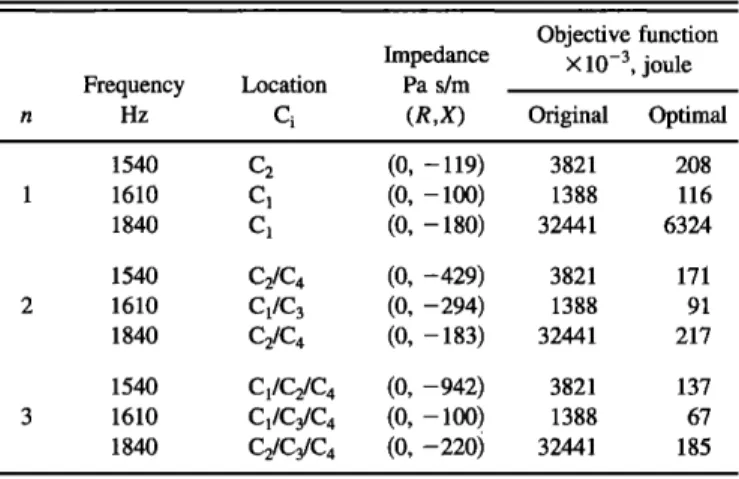
and three configuration; • are simulated, as indicated in Table
I. As previously mentioned, optimal impedances for these cases are generally purely reactive. Also, optimal locations and impedances of acoustical treatments alter with the fre- quency of excitation. If the characteristic of the noise source is a narrow band with the specific resonance of •..cavity, this information can be useful for better acoustical material patching in the preliminary design stage. Performance of us- ing three pieces of acoustical material is deemed more gen- erally effective than that of a single and double one, i.e., a 16% to 97% lower objective function. Table II indicates that the typical history of iterations while location and impedance of acoustical material are simultaneously considered as de- sign variables.
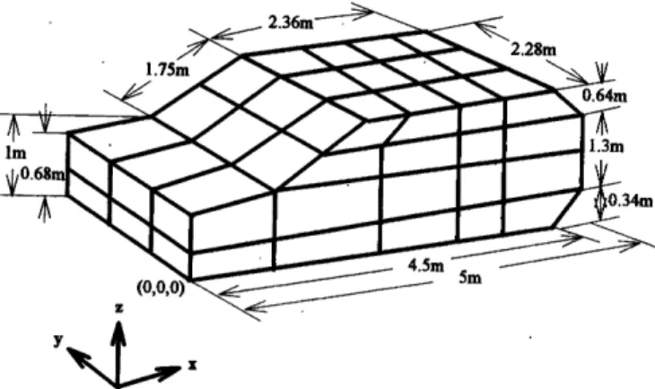
B. Acoustical treatments in an irregularly shaped cavity
A car cabin
of its dimensions
shown
in Fig. 1028
is se-
lected as a practical situation in which an irregularly shaped boundary occurs. The engine firing frequency dominates the internal noise level in a number of cars, particularly at higher
TABLE I. Optimal acoustical treatments in the resonant excitation of the two-dimensional cavity with n = 1, 2, and 3, respectively.
Objective function Impedance X 10 -3, joule Frequency Location Pa s/m n Hz Ci (R,X) Original Optimal 1540 C2 (0, - 119) 3821 208 1610 C 1 (0, -100) 1388 116 1840 C1 (0, - 180) 32441 6324 1540 C2/C 4 (0, -429) 3821 171 1610 C•/C 3 (0, -294) 1388 91 1840 C2/C4 (0, -183) 32441 217 1540 C1/C2/C 4 (0, -942) 3821 137 1610 C1/C3/C 4 (0, - 100) 1388 67 1840 C2/C3/C 4 (0, -220) 32441 185 ,
engine
speeds.
29 Therefore,
control
of engine-induced
noise
inside the car is of vital interest in this study. A frequency range of 20 to 200 Hz is focused upon as a result of the likelihood of a low-frequency, engine noise boom phenom- enon which is increased by the current trend toward lighter car bodies and more powerful engines. The control volume
utilized
to compute
the squared
acoustic
pressure
(p2) of the
objective function is located in the vicinity of the driver's and passengers' heads in the cavity. For convenience, the seats in the cabin are removed, and rigid walls are assumed on the boundary unless otherwise stated. A noise source of
volume
velocity
1 m3/s
is positioned
at (0.5, 0.14, 0.34) to
simply simulate a single transmission path of the engine- induced noise. Five candidate regions are selected for patch- ing acoustical matehals, i.e., roof, floor, left door, right door, and back panels. Design bounds of impedance are 0•<R •< 1000 and 100•<X•<2000 Pa s/m. SPL at passenger heads, i.e., locations of (2.3, 0.6, 1.2), (2.3, 1.4, 1.2), (3.2, 0.6, 1.2), and (3.2, 1.4, 1.2), must be smaller than 80 dB. This SPL value can be practically assigned if the character- istics of the noise source are precisely defined.
First, acoustical influences in the frequency range from 20 to 200 Hz at five regions are verified at specified imped- ance, as shown in Fig. 11. Acoustical influence is defined here as the average insertion loss (IL) in the frequency range of interest. However, the IL is known to be the difference of SPL in the control volume with and without the acoustical treatments. The thickness of the shading near the panel or the number of the dB, indicates the relative influence on the sound pressure reduction of the control volume qualitatively or quantitatively. This reduction is a result of patching acous- tical matehal with fixed impedances to that particular panel across the frequency band of interest. This figure reveals that the major contributing panel to noise reduction is situated in the floor region. Of course, these results depend strongly upon the frequency range, control volume, characteristics of noise source, and specified impedance of acoustical material. However, computations such as these can provide useful in- formation regarding contributing panels at frequencies char- actedzing important excitation of engine firing. From Fig. 11, acoustical influence of the floor panel (region) is obvi- ously more dominant than others, i.e., a 6 to 7 dB higher IL.
In order to more fully comprehend the characteristics of acoustical treatments in the region of floor, a simulation of results shown in Figs. 12 and 13 is conducted. Again, the purely reactive impedance is preferred at the optimal acous- tical treatments in this low frequency range. Reasons for this trend are similar to those mentioned in Sec. III A. However, a lower bound tendency of the optimal reactance can be re- lated to the geometrical configuration of the cavity, position of noise source, and complexity of sound fields in the cabin. Furthermore, effectiveness of acoustical treatments is quite high at the resonant excitation of the car cabin due to a lower objective function (0.4%-6% of original one) and a higher insertion loss (13 dB on average).
Finally, acoustical treatments in the resonant excitation of the car cabin with location and impedance as design vari- ables simultaneously are illustrated in Table III for n = 1, 2
TABLE II. The typical history of iterations while using the location of the acoustical material as a design
variable.
Acoustical treatments for a cavity of dimensions 0.56X0.32X0.08 m The input data file in pnc. inp
NUMBER OF DESIGN VARIABLES --6
NUMBER OF OBJECTIVE FUNCTIONS -1
NUMBER OF EQUALITY CONSTRAINTS -1 NUMBER OF INEQUALITY CONSTRAINTS =0
MAXIMUM NUMBER OF ITERATIONS -100
INDEX OF PRINTING CODE =0
GRADIENT CALCULATION INDICATOR -1 NO. OF CONSECUTIVE ITER. FOR ACT =5 TOL. IN CONSTR. VIOL. AT OPT. = 1.0000e-04
CONVERGENCE PARAMETER VALUE = 1.0000e-04
DEL FOR F. D. GRAD. CALCULATION = 1.0000e-01 ACCEPTABLE CHANGE IN COST FUNC. = 1.0000e-09
ß :::' Type, Starting design and its limits ...
No. Type Design Lower lim Upper lim
1 Zero-one 0.0000e +00 0.0000e +00
2 Zero-one 1.0000e +00 0.0000e +00
3 Zero-one 0.0000e +00 0.0000e +00
4 Zero-one 1.0000e +00 0.0000e +00
5 Continue 0.0(J00e +00 0.0000e +00
6 Continue i.0000e +02 1.0000e +02
First cycle: Initial design:
X[1] 0.0000e +00 X[2] 1.0000e +00 X[3] 0.0000e +00 X[4] 1.0000e +00
X[5] 0.0000e+00 X[6] 1.0000e+02
*** Final design:: ***
*X[1] 0.0000e+00 *X[2] 5.0000e-01 *X[3] 1.0000e+00
*X[4] 5.0000e-01 *X[5] 0.0000e+00 *X[6] 1.9686e+02
*** Cost function at optimum = 1.8992628 e + 02 ***
No. of calls for cost function evaluation (usermf) =700
No. of calls for cost function gradient evaluation (usermg) =0
No. of calls for constraint function evaluation (usercf) =700
No. of calls for constraint function gradients evaluation (usercg) =0
No. of total gradient evaluations = 100
The following cycles are the BRANCH-AND-BOUND cycles:
Initial design:
X[1] 0.0000e +00 X[2] 1.0000e +00 X[3] 5.0000e-01 X[4] 0.0000e +00 X[5] 1.9686e+02
*** Final design:: ***
*X[1] 4.4432e-02 *X[2] 1.0000e+00 *X[3] 9.5557e-01
*X[4] 0.0000e+00 *X[5] 1.9318e+02
*** Cost function at optimum=2.3261524e +02 ***
No. of calls for cost function evaluation (usermf)=71 No. of calls for cost function gradient evaluation (usermg)=0 No. of calls for constraint function evaluation (usercf)=69 No. of calls for constraint function gradients evaluation (usercg)=0 No. of total gradient evaluations=6
1.0000e+00 1.0000e +00 1.0000e+00 1.0000e +00 1.0000e+03 2.0000e+03
TABLE II. (Continued.)
(The middle steps are deleted) Initial design:
X[1] 0.0000e+00 X[2] 0.0000e+00 X[3] 0.0000e+00 X[4] 1.8345e+02
*** Final design:: ***
*X[1] 0.0000e+00 *X[2] 0.0000e+00 *X[3] 0.0000e+00 *X[4] 1.8345e+02 *** Cost function at optimum=2.1746219e +02 ***
No. of calls for cost function evaluation (usermf)=30 No. of calls for cost function gradient evaluation (usermg)=0 No. of calls for constraint function evaluation (usercf)=29 No. of calls for constraint function gradients evaluation (usercf)=0 No. of calls gradient evaluations=2
Final results:
Number of iterations= 1
Maximum constraint violation = 0.00000e + 00
Convergence parameter= 1.48308e-01 The value of supercrition= 2.17462e + 02 The design variables:
X[1] 0.0000e+00 x[2] 1.0000e+00 X[3] 0.0000e+00
X[4] 1.0000e+00 X[5] 0.0000e+00 X[6] 1.8345e+02
Total number of calls of USERMF=2308
Total number of calls of USERMG=0 Total number of calls of USERCF=2304
Total number of calls of USERCG=0
No. of total eval. of grad=386
and 3, respectively. Some remarks can be drawn from these
typical simulations.
(1) The optimal location of acoustical patching for the n = 1 case is all of positioning in the floor region. Also, one of the optimal treatments for all of n =2 and 3 cases contains the floor panel. These results can directly correlate with the analysis of acoustical influence in the aforementioned sec-
tion. ß
(2) In light of dominance of acousti6al treatment in the
floor region, performance of the n =2 and 3 cases does not
have much of an improvement as compared with the n-1
case, except for the resonant excitations of 39 and 66 Hz. (3) However, purely-reactive impedance preferred is not
true for some particular situations. For instance, resistance is
1.75: 2.28m 0.64m 1.3111 0.34m (o,o,o] 5m
FIG. 10. The mesh and dimensions of a car cabin utilized in Sec. III B.
310 d. Acoust. Soc. Am., Vol. 98, No. 1, July 1995
also required
to optimally
attenuate
the noise
at the excita-
tions of 75 and 103 Hz for the n =2 case. This can be as a result of either the objective function being insensitive to the variation of impedance in the neighborhood of global mini- mum or other mechanisms which are not clearly known.
4.2
dB
Roof
ø•
Back Floor' 10.5 dB -'"' ß 3.1 dB 3.5 dB 3.O dB (a) Right door Left doorß -•
(b) .FIG. 11. Acoustical influence diagram: (a) side view, (b) top view.
0 • o o
-tOO
-200 -300X-X-X--
X X (X-XX-X--X• •-X•x Resistance ---x-- Reactance 0 50 tOO 150 200 Frequency (Hz)FIG. 12. Optimal impedance in the region of floor as a function of fre- quency for the car cabin.
(4) Performance for the n = 3 case is not necessarily bet-
ter than that for the n-- 1 and 2 cases as a result of complexi- ties of primary sound fields in the cavity, dominance of acoustical treatment in the floor region, and local minimum searching of the algorithm. This knowledge implies that the number of piece of acoustical materials can be optimized if it is selected as a design variable.
IV. CONCLUSIONS
Combining the numerical BE acoustical analysis with the SQP optimization solver could be an effective tool for designing acoustical treatments in cavities at low frequency. The SQP optimization solver was enhanced in this study by the modified BBM procedure to simultaneously treat the practical applications of continuous and noncontinuous de- sign variables. This would be especially useful while the conventional combinatorial design has become impractical. A small two-dimensional cavity was verified as well as the utility of the proposed design tool demonstrated by an irregu- larly shaped car cabin. Computer simulations indicated that at a low frequency, where enclosures can properly be termed as tightly coupled, purely reactive acoustical treatments are generally preferred at resonances or near-resonances of the two-dimensional cavity as well as at the frequency of interest
1200 1000
800
600400
200 0i
•
original
-->xxxxxx. x- u-XX-xx_xx-x x•x x• 0 50 100 150 200 Frequency (Hz)FIG. 13. Objective function in the region of floor as a function of frequency
for the car cabin.
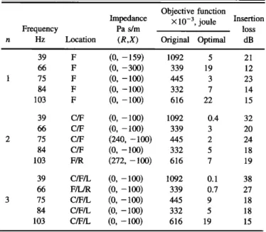
TABLE III. Optimal acoustical treatments in the resonant excitation of the car cabin with n = 1, 2 and 3, where C, F, L, and R represent the regions of ceiling, floor, left, and right door panel, respectively.
Objective function
Impedance X 10
-3, joule Insertion
Frequency Pa s/m loss
n Hz Location (R,X) Original Optimal dB
39 F (0, - 159) 1092 5 21 66 F (0, -300) 339 19 12 1 75 F (0, - 100) 445 3 23 84 F (0, -100) 332 7 14 103 F (0, - 100) 616 22 15 39 C/F (0, - 100) 1092 0.4 32 66 C/F (0, - 100) 339 3 20 2 75 C/F (240, - 100) 445 2 24 84 C/F (0, - 100) 332 5 18 103 F/R (272, - 100) 616 7 19 39 C/F/L (0, - 100) t 092 0.1 38 66 F/L/R (0, - 100) 339 0.7 27 3 75 C/F/L (0, -100) 445 9 18 84 C/F/L (0, - 100) 332 5 18 103 C/F/L (0, - 100) 616 19 15
in the car cabin. This general agreement between the present
study
and the previous
work of Bernhard
and Takeo
7 was
considered adequate for the proposed tool to be utilized for the preliminary design study of acoustical treatments in en- closures. Furthermore, the optimal locations of acoustical treatments would always contain the region of dominant acoustical influence in the situation of multiple patching. However, capability of optimizing locations and impedances of acoustical material simultaneously were not considered in the previous work.
ACKNOWLEDGMENTS
The authors acknowledge the National Science Council, Taiwan, R.O.C. for partial support of this work under grant
NSC 82-0401-E009-085. The Center for Measurement Stan-
dards of Industrial Technology Research Institute, Taiwan, R.O.C. is also appreciated for financially supporting T. C. Yang.
1D. Y. Maa, "Theory and Design of Microperoforated Panel Sound-
Absorbing Constructions," Sci. Sinica 18, 55-71 (1975).
D. Y. Maa, "Microperoforated Panel Wideband Absorbers," Noise Control
Eng. J. 29 (3), 77-84 (1987).
3j. Lee and G. W. Swenson, Jr., "Compact Sound Absorbers for Low
Frequencies," Noise Control Eng. J. 38 (3), 109-117 (1992).
4R. S. Jackson, "The Performance of Acoustic Hoods at Low Frequen-
cies," Acusfica 12, 139-152 (1962).
M. C. Junger, "Sound Transmission Through an Elastic Enclosure Acous-
tically Closely Coupled to a Noise Source," ASME Paper No. 70-WA/ DE-t2 (1970).
L. W. Tweed and D. R. Tree, "Three Methods for Predicting the Insertion
Loss of Close-Fitting Acoustical Enclosures," Noise Control Eng. 10 (2), 74-79 (1978).
7R. J. Bernhard and S. Takeo, "A Finite Element Procedure for Design of Cavity Acoustical Treatments," J. Acoust. Soc. Am. 83, 2224-2230 (1988).
8j. S. Arora, Introduction to Optimum Design (McGraw-Hill, New York,
1989).
9C. H. Tseng, L. W. Wang, and S. E Ling, "Numerical Study of Branch-
and-Bound Method in Structural Optimization," Technical Report AODL-
90-02, National Chiao Tung University, Taiwan, ROC (1990).
løC. H. Tseng, L. W. Wang, and S. E Ling, "Enhancing the Branch-and-
Bound Structural Optimization," Proc. Int. Conf. Comput. Methods Eng.,
Singapore, 1180-1185 (1992).
• C. H. Tseng, L. W. Wang, and S. F. Ling, "Enhancing the Branch-and-
Bound Method for Structural Optimization," to appear in the ASCE J. Struct. Eng. (1995).
12L. H. Chen and D. G. Schweikert, "Sound Radiation from an Arbitrary Body," J. Acoust. Soc. Am. 35, 1626-1632 (1963).
13 R. D. Ciskowski and C. A. Brebbia, Boundary Element Methods in Acous- tics (Elsevier Applied Science, London, 1991).
14L. E. Kinsler, A. R. Frey, A. B. Coppens, and J. V. Sanders, Fundamentals of Acoustics. (Wiley, New York, 1982).
•5 A. Craggs, "A Finite Element Method for Modeling Dissipative Mufflers with a Locally Reactive Lining," J. Sound Vib. 54 (2), 285-296 (1977). •6C. H. Jo and S. J. Elliott, "Active Control of Low Frequency Sound
Transmission Between Rooms," J. Acoust. Soc. Am. 92, 1461-1472 (1992).
•7 C. G. Mollo and R. J. Bernhard, "Generalized Method of Predicting Op-
timal Performance of Active Noise Controllers," AIAA J. 27 (11), 1473- 1478 (1989).
•8M. Tanaka, Y. Yamada, and M. Shirotori, "Boundary Element Method
Applied to Simulation of Active Noise Control in Ducts," JSME Int. J. 35 (3), 387-392 (1992).
19 K. A. Cunefare and G. H. Koopmann, "A Boundary Element Approach to
Optimization of Active Noise Control Sources on Three-Dimensional Structures," ASME J. Vib. Acoust. 113, 387-394 (1991).
2øT. C. Yang, C. H. Tseng, and C. H. Huang, "An Interface Coupler for
Finite Element Analysis and Optimization," Proc. Sixteenth National Conf. Theoretical and Applied Mechanics, Keelung, Taiwan, ROC, 887- 894 (1992).
2•T. C. Yang, C. H. Tseng and S. F. Ling, "Constrained Optimization of
Active Noise Control Systems in Enclosures," J. Acoust. Soc. Am. 95, 3390-3399 (1994).
22C. H. Tseng and J. S. Arora, "On Implementation of Computational Al-
gorithms for Optimal Design, Part I: Preliminary Investigation," Int. J. Num. Methods Eng. 26, 1365-1384 (1988).
23 C. H. Tseng and J. S. Arora, "On Implementation of Computational Al-
gorithms for Optimal Design, part II: Extensive Numerical Investigation," Int. J. Num. Methods Eng. 26, 1385-1402 (1988).
24C. U. Tseng and W. C. Liao, "Integrated Software for Multifunctional
Optimization," Tech. Report AODL-90-01, Dept. of Mechanical Eng., Na- tional Chiao Tung Univ., Taiwan, ROC (1990).
25 B. N. Pshenichny, "Algorithms for the General Problem of Mathematical Programming," Kibemetica, No. 5 (1978).
26 A.D. Belegundu and J. S. Arora, "A Recursive Quadratic Programming
Algorithm with Active Set Strategy for Optimal Design," Int. J. Num. Methods Eng. 20, 803-816 (1984).
27 M. C. Junger and D. Feit, Sound, Structures, and Their Interaction (MIT,
Cambridge, 1986).
28M. R. Bai, "Study of Acoustic Resonance in Enclosures Using Eigenan- alysis Based on Boundary Element Methods," J. Acoust. Soc. Am. 91,
2529-2538 (1992).
29p. A. Nelson and S. J. Elliott, Active Noise Control of Sound (Academic,
London, 1992).