Research Article
A Computer-Aided Approach to Pozzolanic Concrete Mix Design
Ching-Yun Kao ,
1Chin-Hung Shen,
2Jing-Chi Jan,
3and Shih-Lin Hung
41Associate Professor, Department of Applied Geoinformatics, Chia Nan University of Pharmacy & Science, No. 60,
Sec. 1, Erh-Jen Rd., Tainan 71710, Taiwan
2Graduate Student, Department of Civil Engineering, National Chiao Tung University, No. 1001, University Rd.,
Hsinchu 300, Taiwan
3Associate Professor, Department of Computer Science and Information Engineering, Chien Hsin University of Science and
Technology, No. 229, Jianxing Rd., Zhongli Dist., Taoyuan City 32097, Taiwan
4Professor, Department of Civil Engineering, National Chiao Tung University, No. 1001, University Rd., Hsinchu 300, Taiwan
Correspondence should be addressed to Shih-Lin Hung; [email protected] Received 30 May 2018; Accepted 2 September 2018; Published 10 October 2018 Guest Editor: Maksym Grzywinski
Copyright © 2018 Ching-Yun Kao et al. This is an open access article distributed under the Creative Commons Attribution License, which permits unrestricted use, distribution, and reproduction in any medium, provided the original work is properly cited.
Pozzolanic concrete has superior properties, such as high strength and workability. The precise proportioning and modeling of the concrete mixture are important when considering its applications. There have been many efforts to develop computer-aided approaches for pozzolanic concrete mix design, such as artificial neural network- (ANN-) based approaches, but these approaches have proven to be somewhat difficult in practical engineering applications. This study develops a two-step computer-aided approach for pozzolanic concrete mix design. The first step is establishing a dataset of pozzolanic concrete mixture proportioning which conforms to American Concrete Institute code, consisting of experimental data collected from the literature as well as numerical data generated by computer program. In this step, ANNs are employed to establish the prediction models of compressive strength and the slump of the concrete. Sensitivity analysis of the ANN is used to evaluate the effect of inputs on the output of the ANN. The two ANN models are tested using data of experimental specimens made in laboratory for twelve different mixtures. The second step is classifying the dataset of pozzolanic concrete mixture proportioning. A classification method is utilized to categorize the dataset into 360 classes based on compressive strength, pozzolanic admixture replacement rate, and material cost. Thus, one can easily obtain mix solutions based on these factors. The results show that the proposed computer-aided approach is convenient for pozzolanic concrete mix design and practical for engineering applications.
1. Introduction
Concrete plays an important role in the growing con-struction industry. Presently, various types of by-product materials, such as fly ash, silica fume, rice husk ash, and others have been widely used as pozzolanic materials in concrete. Studies [1–4] have shown that utilization of pozzolanic material not only improves concrete properties (such as strength and durability) but also helps to preserve the environment. Moreover, superplasticizers play a crucial role in the development of high strength and high-performance concrete. Superplasticizers are admixtures which are added to concrete mixture in very small dosages. Their addition results in a significant increase in the
workability of the mixture, as well as a reduction of water/cement ratio and of cement quantity [5].
Several researchers have looked into the characteristic parameters that affect the compressive strength and slump of conventional and high-strength concrete [6–8]. These parameters typically include water, cement, coarse aggre-gate, and fine aggregate. Conventional methods initially involve constructing a mathematical model, which is fol-lowed by a regression analysis using experimental data to determine unknown coefficients in that model and es-tablish correlations between these parameters and com-pressive strength and slump. Conventional methods generally include complex modeling and are inappropriate where experimental data are imprecise and parameters
Volume 2018, Article ID 4398017, 15 pages https://doi.org/10.1155/2018/4398017
affecting compressive strength and slump are incomplete in the experimental data.
Artificial neural networks (ANNs) were originally de-veloped to simulate the function of the human brain or neural system. Subsequently, they have been widely applied to diverse fields, ranging from biology to many engineering fields. ANNs exhibit a number of desirable properties not found in conventional symbolic computation systems, in-cluding robust performance when dealing with noisy or incomplete input patterns, a high degree of fault tolerance, high parallel computation rates, the ability to generalize, and adaptive learning [9–11]. ANNs are capable of modeling input-output functional relations, even when mathemati-cally explicit formulas are unavailable. Therefore, ANNs are suitable for prediction of compressive strength and slump of concrete. Accordingly, the feasibility of applying ANNs to predict compressive strength and slump of concrete has received considerable attention. Yeh [12] investigated the potential of using design of experiments and ANNs to determine the effect of fly ash replacements on early and late compressive strength of low- and high-strength concrete. Yeh [13] further demonstrated the possibilities of adapting ANNs to predict the compressive strength of high-performance concrete. Kasperkiewics et al. [14] applied ANNs to predict the 28-day compressive strength of high-performance concrete composed of six components (ce-ment, silica, superplasticizer, water, fine aggregate, and coarse aggregate). Lee [15] used ANNs to predict the compressive strength development of concrete. Bai et al. [16] developed neural network models to predict the workability of concrete incorporating metakaolin and fly ash. Duan et al. [17] applied ANNs to predict the compressive strength of recycled aggregate concrete. Ni and Wang [18] developed a method to predict 28-day compressive strength of concrete by using ANNs based on the inadequacy of methods dealing with multiple variable and nonlinear problems.
In light of the above developments, this study develops a two-step computer-aided approach for pozzolanic con-crete mix design. The first step is establishing the dataset of pozzolanic concrete mixture proportioning which conform to American Concrete Institute (ACI) code. The dataset consists of experimental data collected from the literature and numerical data generated by computer program. In this step, ANNs are employed to establish the prediction models of compressive strength and slump of concrete. Sensitivity analysis of the ANN is used to evaluate the effect of inputs on the output of the ANN. The two ANN models are tested using data of experimental specimens made in laboratory for twelve different mixtures. The second step is classifying the dataset of pozzolanic concrete mixture proportioning. A classification method is utilized to categorize the dataset into 360 classes based on compressive strength of concrete, pozzolanic admixture replacement rate, and cost of the concrete.
2. Artificial Neural Networks
ANNs form a class of systems that are inspired by biological neural networks. The topology of an ANN model consists of
a number of simple processing elements, called nodes, which are interconnected to each other. Interconnection weights that represent the information stored in the system are used to quantify the strength of the interconnections; these weights hold the key to the functioning of an ANN.
2.1. Back-Propagation Neural Networks. Among the many
different types of ANN, by far the most commonly applied neural network learning model, due to its simplicity, is the feedforward, multilayered, supervised neural network with error propagation algorithm, the so-called back-propagation (BP) network [11]. Before an ANN can be used in an application, it must either learn or be trained from an existing database consisting of pairs of input-output patterns. The topology of BP networks consists of an in-put layer, one or more hidden layers, and an outin-put layer. The training of a supervised neural network usually involves three stages. The first stage is the data feedforward. The output of each node is defined as follows:
netj� n i�1 WijOi+θj, Oj� fnetj, (1)
where Wijis the weight associated with the ith node in the preceding layer to the jth node in the current layer; Oiis the output of ith node in the preceding layer; θjis the threshold value of node j in the current layer; Ojis the output of node j in the current layer; and function f is the activation function, which has to be differentiable. Herein, the hyperbolic tan-gent function is used as the activation function and is defined as follows:
f(x) �e
x− e−x
ex+ e−x. (2) The second stage is error back-propagation and ad-justment of the network weights. The training process ap-plies mean square error (E), the absolute fraction of variance (R2), and sum of the squares error (SSE), to monitor the learning performance of the network. E, R2, and SSE are defined, respectively, as E �1 P P p�1 K k�1 dpk− opk 2, R2�1 − P p�1 K k�1dpk− opk 2 Pp�1Kk�1opk2 , SSE � P p�1 K k�1 dpk− opk 2, (3)
where P denotes the number of instances in the training set, while dpk and opk represent the desired and calculated output of the kth output node for the pth instance, re-spectively. The standard BP algorithm employs a gradient descent approach with a constant step length (learning ratio) to train the network.
Wij,k+1� Wij,k+ΔWij,
ΔWij�−η zE
zWij,
(4)
where η is the learning ratio, which is a constant in the range of [0, 1]. The suffix index k denotes the kth learning iteration. Unfortunately, BP supervised neural network learning models require a significant amount of time to learn. Moreover, the convergence of a BP neural network is highly dependent upon the use of a learning rate (η). Consequently, several different approaches are developed here to enhance the learning performance of the BP learning algorithm [10].
Hung and Lin [19] developed a more effective adaptive limited memory Broyden–Fletcher–Goldfarb–Shanno (L-BFGS) learning algorithm based on the approach of a L-BFGS quasi-Newton second-order method [20, 21] with an inexact line search algorithm. This algorithm achieved a superior convergence rate to the BP learning algorithm by using second-order derivatives of the system error function with respect to the network weights. In the conventional BFGS method, the approximation Hk+1 to the inverse Hessian matrix of function E(W) is updated by
Hk+1� I − ρksky T k Hk I − ρkyks T k +ρksks T k ≡ VTkHkVk+ρksks T k, (5) where ρk� 1 yT ksk , Vk�I − ρkyks T k, sk�Wk+1− Wk, yk�gk+1− gk, gk� zE zW. (6)
Instead of forming the matrix Hkwith the BFGS method, the vectors skand ykare saved. These vectors first define and then implicitly and dynamically update the Hessian ap-proximation using information from the last few iterations, referred to here as m. Therefore, the final stage of the ad-justment of the weights in a BP-based ANN is modified as follows:
Wk+1�Wk+αkdk. (7)
The search direction is given by
dk�−Hkgk+βkdk−1, (8) where βk� yT (k− 1)H(k−1)g(k−1) yT (k− 1)d(k−1) . (9)
The step length, αk, is adapted during the learning process through a mathematical approach: the inexact line search algorithm. This approach is used in the L-BFGS learning algorithm instead of a constant learning ratio [19]. The inexact line search algorithm is based on three se-quential approaches: bracketing, sectioning, and in-terpolation. The bracketing approach brackets the potential step length, α, between two points, through a series of function evaluations. The sectioning approach then uses the two points of the bracket as the initial points, reducing the step size, and locating the minimum between points, such as,
α1 and α2, to a specified degree of accuracy. Finally, the quadratic interpolation approach uses the three points, α1,
α2, and (α1+ α2)/2, to fit a parabola to determine the step length, αk. Consequently, the step length αkmust satisfy the following conditions in each iteration [19]:
E Wk+αkdk≤ E Wk +βαk ∇E Wk T dk β ∈ (0, 1) and αk> 0, ∇E Wk+αkdk T dk≥ θ ∇E Wk T dk θ ∈ (β, 1) and αk> 0, ∇E Wk+αkdk T d(k+1)< 0. (10) The problem of selecting a learning ratio through trial and error in the BP algorithm is thus circumvented in the adaptive L-BFGS learning algorithm.
2.2. Architectures of ANN Models. The ANN models,
com-pressive strength prediction neural network (CSPNN) and slump prediction neural network (SPNN), are used in this study for prediction of the 28-day compressive strength (abbreviated below as compressive strength) and slump of pozzolanic concrete, respectively. The architectures of the CSPNN and SPNN are illustrated in Figure 1. Both CSPNN and SPNN developed in this study have seven neurons in the input layer and one neuron in the output layer. The inputs of both CSPNN and SPNN are water, cement, ground gran-ulated blast furnace slag (GGBFS), fly ash, coarse aggregate (CA), fine aggregate (FA), and superplasticizer (SP). The outputs of CSPNN and SPNN are compressive strength (fc′) and slump (S), respectively. Table 1 shows the minimum and maximum values of the seven input parameters used in CSPNN and SPNN.
2.3. Sensitivity Analysis. Cybenko [22] and Funahashai [23]
rigorously demonstrated that even with only one hidden layer, neural networks can uniformly approximate any continuous function. Although neural networks can find a relationship between the input and output values in-ternally, it is not always easy to interpret the resulting weight state. Thus, the effect of one input parameter on the output is difficult to analyze. Alternatively, it is possible to compute the sensitivity of the output value with respect to one of its inputs by taking the first-order partial derivative [24, 25].
If there is a network with n hidden layers, the output of the kth node in the output layer is defined as follows:
Ok� f netok, netok�
j
Whnj,okHnj+θok, (11)
where Hnjis the output of the jth node in the nth hidden layer, θokis the threshold value of the kth node in the output layer, Whnj,okis the weight associated with the jth node in the
nth hidden layer to the kth node in the output layer, and
function f is the activation function.
The first-order partial derivative of the kth output with respect to ith input D1kican be derived as follows:
D1ki�zOk zXi � jn , . . . , j1
Whnjn,okf′ netok, . . . , Wxi,h1j1f′neth1j1, (12) where Wxi,h1j1is the weight associated with the ith node in the input layer to the j1th node in the first hidden layer and
Whnjn,okis the weight associated with the jnth node in the
nth hidden layer to the kth node in the output layer.
Equation (12) indicates that D1
ki is a function of weights, threshold value, and the first-order derivative of the acti-vation function (or a function of weights, threshold values, and training instances). Since D1kiis a function of training instances, generally, the mean of D1kifor the entire training instances can be used to describe the nominal value of the
sensitivity of the kth output parameter with respect to the
ith input parameter. The mean of D1
kifor the entire training instances is D1ki�1 P P p�1 D1ki,p, (13)
where D1ki,pis the value of D1kiof the pth training instance, and P is the total number of training instances. In fact, D1ki can represent the correlation between the kth output pa-rameter and the ith input papa-rameter. A positive (negative) value of D1kirepresents a positive (negative) correlation. The absolute value of D1ki represents the strength of the corre-lation. A larger absolute value of D1ki represents a stronger correlation. Absolute values of D1kinear zero indicate little or no correlation.
3. Proposed Approach for Pozzolanic Concrete
Mix Design
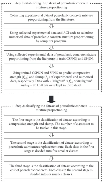
This study develops a computer-aided approach for poz-zolanic concrete mix design. This approach is suitable for designing a mix of pozzolanic concrete with compressive strength, fc′, from 210 kgf/cm2to 980 kgf/cm2and slump, S, equal to 20 cm. As shown in Figure 2, this approach involves two steps. The first step is establishing the dataset of poz-zolanic concrete mixture proportioning that conform to ACI code, consisting of experimental data collected from liter-ature and numerical data generated by computer program. The second step is classifying the dataset of pozzolanic concrete mixture proportioning. A classification method is utilized to categorize data into 360 clusters according to compressive strength of concrete, pozzolanic admixtures replacement rate, and material cost. The following presents the details of the proposed approach.
3.1. Establishing the Dataset of Pozzolanic Concrete Mixture Proportioning. As shown in Figure 2, the process of
establishing the dataset of pozzolanic concrete mixture proportioning is listed as follows:
(1) Collecting experimental data of pozzolanic concrete mixture proportioning from the literature [3, 26–38].
Water Cement Ground granulated blast furnace slag
Fly ash Coarse aggregate Fine aggregate Superplasticizer Compressive strength (a) Water Cement Ground granulated blast furnace slag
Fly ash Coarse aggregate Fine aggregate Superplasticizer Slump (b)
Figure 1: The architectures of (a) CSPNN and (b) SPNN.
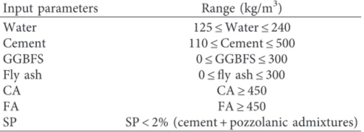
Table 1: Range of input parameters of CSPNN and SPNN in dataset.
Input parameters Range (kg/m3)
Water 125 ≤ Water ≤ 240
Cement 110 ≤ Cement ≤ 500
GGBFS 0 ≤ GGBFS ≤ 300
Fly ash 0 ≤ fly ash ≤ 300
CA CA ≥ 450
FA FA ≥ 450
(2) Generating numerical data of pozzolanic concrete mixture proportioning since the collected experi-mental data may be insufficient. Before generating numerical data, the ranges of material contents (as listed in Table 1) are set based on collected experi-mental data of pozzolanic concrete mixture pro-portioning and ACI code for pozzolanic concrete mix design (as listed in Tables 2–8) [39]. Numerical data of pozzolanic concrete mixture proportioning are then generated randomly using the ACI mix design method for pozzolanic concrete (as shown in Figure 3). (3) Using a portion of collected experimental data of
pozzolanic concrete mixture proportioning to train CSPNN and SPNN. The effect of input parameters on the output is evaluated by sensitivity analysis. The prediction accuracy of CSPNN and SPNN is tested using the remainder of the collected experimental
data and data from experimental specimens made in our laboratory for twelve different mixtures. (4) Using trained CSPNN and SPNN to predict
com-pressive strength and slump of experimental and numerical data, respectively. Data that satisfy the following conditions are kept in the dataset.
210 kgf/cm2≤ fc,CSPNN′ ≤ 980 kgf/cm 2, 20 + 3.8 cm ≤ SSPNN≤ 20 − 3.8 cm,
(14)
where fc,CSPNN′ and SSPNN are compressive strength and slump predicted by CSPNN and SPNN, respectively. The reasons for this are (1) this approach is suitable for mixing design of pozzolanic concrete with compressive strength, fc′, from 210 kgf/cm2to 980 kgf/cm2and slump, S, equal to 20 cm, and (2) the allowable data range width of slump in Taiwan is set to be 3.8 cm when slump is larger than 10 cm [40].
3.2. Classifying the Dataset of Pozzolanic Concrete Mixture Proportioning. To produce a dataset of pozzolanic concrete
mixture proportioning which is more feasible and conve-nient for engineering applications, it is classified further.
In classification, a sampling unit (subject or object) whose class membership is unknown is assigned to a class on the basis of the vector, y, associated with the unit. To classify the unit, we must have available a previously obtained sample of observation vectors from each class. One approach is to then compare y with the mean vectors y1, y2,. . ., ykof the k classes and assign the unit to the class whose yi is closest to y [41]. Many techniques use an index of similarity or proximity between y and yi. A convenient measure of proximity is the distance. The distances used in classification algorithms include Euclidean distance, Manhattan distance, Chebyshev distance, Minkowski distance, and Mahalanobis distance. Since Euclidean distance is the most well-known distance, it is applied in this study. The Euclidean distance between two vectors (points) a and b is defined as
dis(a, b) � ����������� j aj− bj 2 , (15)
where ajand bj are the jth element of a and b, respectively. The proposed classification of the dataset of pozzolanic concrete mixture proportioning is according to compressive strength, pozzolanic admixture replacement rate, and cost. As shown in Figure 2, the classification method used in this study involves three stages. The first stage is the classification of dataset according to compressive strength and slump. The number of classes is set as twelve in this stage. The mean (designed) values of compressive strength of the twelve classes are increased from 210 kgf/cm2 (20.6 MPa) to 980 kgf/cm2 (96.1 MPa) every 70 kgf/cm2(6.8 MPa). The mean (designed) values of slump of all twelve classes are the same and are equal to 20 cm. According to the related code in Taiwan, the allowable data range width of compressive strength and slump is 3.4 MPa and 3.8 cm, re-spectively. Thus, the classification rule can be written as
Step 1: establishing the dataset of pozzolanic concrete mixture proportioning
The first stage is the classification of dataset according to compressive strength and slump. The number of class is set to
be twelve in this stage.
The second stage is the classification of dataset according to pozzolanic admixtures replacement rate. Each class in the first
stage is divided into five smaller classes
Collecting experimental data of pozzolanic concrete mixture proportioning from the literature.
Using collected experimental data and ACI code to calculate numerical data of pozzolanic concrete mixture proportioning
by computer program.
Using trained CSPNN and SPNN to predict compressive strength (f′c,p) and slump (Sp) of experimental and numerical
data, respectively. Data with 210 kg/cm2 ≤ f′
c,p ≤ 980 kg/cm2
and Sp = 20±3.8 cm were kept in the dataset.
Using collected experimental data of pozzolanic concrete mixture proportioning from the literature to train CSPNN and SPNN.
The third stage is the classification of dataset according to the cost of pozzolanic concrete. Each class in the second stage is
divided into six smaller classes. Step 2: classifying the dataset of pozzolanic concrete
mixture proportioning
Figure 2: Schematic diagram of the proposed approach for poz-zolanic concrete mix design.
Table 2: Cementitious materials requirements for concrete exposed to deicing chemicals “Table 2 is reproduced from Kosmatka et al. [39] (under the creative commons attribution license/public domain).”
Cementitious materials Maximum percent of total cementitious
materials by mass
Fly ash and natural pozzolans 25
Slag 50
Silica fume 10
Total of fly ash, slag, silica fume, and natural pozzolans 50
Total of natural pozzolans and silica fume 35
Table 3: Approximate mixing water and target air content requirements for different slumps and nominal maximum sizes of aggregate “Table 3 is reproduced from Kosmatka et al. [39] (under the creative commons attribution license/public domain).”
Slump (mm) or air content
Water, kilograms per cubic meter of concrete, for indicated sizes of aggregate
(kg/m3) 9.5 mm 12.5 mm 19 mm 25 mm 37.5 mm 50 mm 75 mm 150 mm Non-air-entrained concrete 25 to 50 207 199 190 179 166 154 130 113 75 to 100 228 216 205 193 181 169 145 124 150 to 175 243 228 216 202 190 178 160 –
Approximate amount of entrapped air in
non-air-entrained concrete (%) 3 2.5 2 1.5 1 0.5 0.3 0.2
Air-entrained concrete
25 to 50 181 175 168 160 150 142 122 107
75 to 100 202 193 184 175 165 157 133 119
150 to 175 216 205 197 184 174 166 154 –
Recommended average total air content, percent, for level of exposure:
Mild exposure 4.5 4.0 3.5 3.0 2.5 2.0 1.5 1.0
Moderate exposure 6.0 5.5 5.0 4.5 4.5 4.0 3.5 3.0
Severe exposure 7.5 7.0 6.0 6.0 5.5 5.0 4.5 4.0
Table 4: Bulk volume of coarse aggregate per unit volume of concrete “Table 4 is reproduced from Kosmatka et al. [39] (under the creative commons attribution license/public domain).”
Nominal maximum size of aggregate (mm)
Bulk volume of dry-rodded coarse aggregate per unit volume of concrete for different fineness moduli of fine aggregate
2.40 2.60 2.80 3.00 9.5 0.50 0.48 0.46 0.44 12.5 0.59 0.57 0.55 0.53 19 0.66 0.64 0.62 0.60 25 0.71 0.69 0.67 0.65 37.5 0.75 0.73 0.71 0.69 50 0.78 0.76 0.74 0.72 75 0.82 0.80 0.78 0.76 150 0.87 0.80 0.83 0.81
Table 5: Relationship between water to cementitious material ratio and compressive strength of concrete “Table 5 is reproduced from Kosmatka et al. [39] (under the creative commons attribution license/public domain).”
Compressive strength at 28 days (MPa) Water-cementitious materials ratio (by mass)
Non-air-entrained concrete Air-entrained concrete
45 0.38 0.30 40 0.42 0.34 35 0.47 0.39 30 0.54 0.45 25 0.61 0.52 20 0.69 0.60 15 0.79 0.70
if disp,i� �������������������� fc,p′ − fc,i′ 2+ S p− Si2 ≤ 5.10 then classp� i(i �1, 2, . . . , 12),
else classp�null,
(16)
where fc,p′ and Spare the compressive strength and slump of the pth instance in the dataset, respectively; fc,i′ and Siare the mean (designed) compressive strength and mean (designed) slump of the ith class, respectively; dp,i is the Euclidean distance between the vector associate to the pth instance in the dataset, yp� (fc,p′ , Sp), and mean vector of class i,
yi� (fc,i′ , Si); and classpis the class the pth instance in the database belongs to.
The second stage is the classification of dataset according to pozzolanic admixtures replacement rate. Pozzolanic ad-mixtures may be used as a partial replacement of cement in
concrete. The pozzolanic admixtures used in this study are fly ash and ground granulated blast furnace slag. Pozzolanic admixture replacement rate, RPA, is expressed as follows:
RPA� PA
PA + cement×100%, (17)
where PA is pozzolanic admixtures. Each class in the first stage is divided into five smaller classes. The class intervals of
RPA are 0–≤10%, >10%–≤20%, >20%–≤30%, >30%–≤40%, and >40%–≤50%.
The third stage is the classification of dataset according to the cost of pozzolanic concrete. Each class in the second stage is divided into six smaller classes. The class intervals of the cost of pozzolanic concrete are 0 (NTD/m3)–≤2000 (NTD/m3), >2000 (NTD/m3)–≤2250 (NTD/m3), >2250 (NTD/m3)–≤2500 (NTD/m3), >2500 (NTD/m3)–≤2750 (NTD/m3), >2750 (NTD/m3)–≤3000 (NTD/m3), and >3000 Table 6: Maximum water-cementitious material ratios and minimum design strengths for various exposure conditions “Table 6 is reproduced from Kosmatka et al. [39] (under the creative commons attribution license/public domain).”
Exposure condition Maximum water-cementitious material ratio
by mass for concrete
Minimum design compressive strength, fc′
(Mpa) Concrete protected from exposure to freezing
and thawing, application of deicing chemicals, or aggressive substances
Select water-cementitious material ratio on basis of strength, workability, and finishing
needs
Select strength based on structural requirements
Concrete intended to have low permeability
when exposed to water 0.50 28
Concrete exposed to freezing and thawing in
a moist condition or deicers 0.45 31
For corrosion protection for reinforced concrete exposed to chlorides from deicing salts, salt water, brackish water, sea water, or spray from these sources
0.40 35
Table 7: Recommended slumps for various types of construction “Table 7 is reproduced from Kosmatka et al. [39] (under the creative commons attribution license/public domain).”
Concrete construction Slump (mm)
Maximum Minimum
Reinforced foundation walls and footings 75 25
Plain footings, caissons, and substructure walls 75 25
Beams and reinforced walls 100 25
Building columns 100 25
Pavements and slabs 75 25
Mass concrete 75 25
Table 8: Requirements for concrete exposed to sulfates in soil or water “Table 8 is reproduced from Kosmatka et al. [39] (under the creative commons attribution license/public domain).”
Sulfate exposure
Water-soluble sulfate
(SO4) in soil, percent by
mass
Sulfate (SO4)
in water, ppm Cement type
Maximum water-cementitious material ratio, by mass Minimum design compressive strength, fc′ (MPa)
Negligible Less than 0.10 Less than 150 No special type required – –
Moderate 0.10 to 0.20 150 to 1500
II, MS, IP(MS), IS(MS), P (MS), I(PM) (MS), I(SM) (MS) 0.50 28 Severe 0.20 to 2.00 1500 to 10,000 V, HS 0.45 31 Very
(NTD/m3). There are 360 classes overall in the dataset of pozzolanic concrete mixture proportioning.
4. Results and Discussion
4.1. ANN-Based Compressive Strength Prediction Model: CSPNN
4.1.1. Training and Testing of the CSPNN Using Collected Experimental Data. All 482 samples collected were used to
train and test the CSPNN. Among the 482 samples, 462 and 20 samples were used to train and test CSPNN, respectively. Here, the CSPNN is constructed with seven, fourteen, and one nodes in input layer, hidden layer, and output layer, respectively, and denoted as CSPNN(7-14-1). The complete offline training process took 47 cycles. The E and R2 were 0.005988 and 0.92556, respectively. After the CSPNN was trained on the 462 training samples, it was tested to observe how accurately it would predict compression strength of other samples. Table 9 and Figure 4 summarize the results of these tests, indicating that the CSPNN can satisfactorily predict the compression strength in all 20 testing samples.
4.1.2. Sensitivity Analysis of the CSPNN. Figure 5 shows the
distribution of compressive strength and water for the training samples of the CSPNN. It shows that compressive strength decreases with increasing amounts of water in the concrete mixture. Compressive strength is inversely pro-portional to water content, and the slope of the fitted simple
regression line is −0.123. Figure 6 shows the distribution of water and the first-order partial derivative of compressive strength with respect to water for the training samples of the CSPNN, and its mean is −0.092. The negative mean value of the first-order partial derivative of compressive strength with respect to water indicates a negative correlation be-tween compressive strength and water, which is consistent with the negative slope value of the fitted simple regression line in Figure 5.
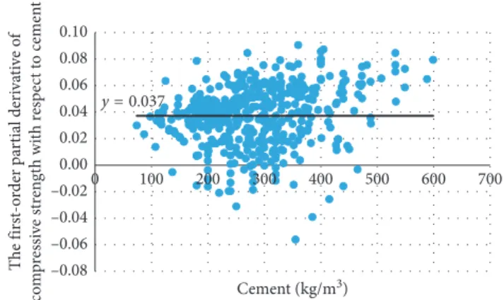
Figure 7 shows the distribution of compressive strength and cement for the CSPNN training samples. It shows that compressive strength increases with an in-crease in the amount of cement in the concrete mixture. Compressive strength is proportional to cement, and the slope of the fitted simple regression line is 0.0764. Figure 8 shows the distribution of cement and the first-order partial derivative of compressive strength with respect to cement for the CSPNN training samples, where the mean is found to be 0.037. The positive mean value of the first-order partial derivative of compressive strength with respect to cement indicates a positive correlation between compressive strength and cement, which is consistent with the positive slope value of the fitted simple regression line in Figure 7.
Figure 9 shows a similar distribution of compressive strength and SP for the CSPNN training samples. Com-pressive strength increases with an increase in the amount of SP in the concrete mixture. Compressive strength is pro-portional to SP, and the slope of the fitted simple regression line is 1.6298. Figure 10 shows the distribution of SP and the first-order partial derivative of compressive strength with respect to SP for the CSPNN training samples. The mean of the first-order partial derivative of compressive strength
Selection of mixture characteristics Start Selection of slump Selection of nominal maximum aggregate size Estimation of water-cement ratio or water-cementitious material ratio Estimation of mixing
water, air, and superplasticize content Selection of the proportion of each pozzolanic material to total cementitious materials Estimation of cement and pozzolanic materials content Estimation of coarse aggregate content Estimation of fine aggregate content Adjustment of mix proportions for the field
conditions
End Mixing
Figure 3: The flow chart of ACI mix design method.
Table 9: Comparison of exact compressive strength with CSPNN-predicted compressive strength for the 20 testing samples.
No. of sample Exact compressive strength (fc,e′) (MPa) Predicted compressive strength (fc,CSPNN′ ) (MPa) fc,e′-fc,CSPNN′ (MPa) 1 57.67 54.93 2.74 2 67.06 58.74 8.32 3 54.90 51.92 2.98 4 41.67 41.12 0.54 5 57.45 58.72 −1.27 6 51.08 52.51 −1.43 7 60.70 62.97 −2.27 8 44.70 38.17 6.53 9 24.20 16.85 7.35 10 46.14 54.93 −8.79 11 44.62 40.39 4.23 12 40.80 44.19 −3.39 13 25.00 30.28 −5.28 14 57.00 59.32 −2.32 15 77.00 70.62 6.38 16 69.00 65.30 3.70 17 64.00 57.01 6.99 18 84.30 85.01 −0.71 19 78.10 75.91 2.19 20 59.00 59.52 −0.52
with respect to SP for the training samples of the CSPNN is 0.087. The positive mean value of the first-order partial derivative of compressive strength with respect to SP in-dicates positive correlation between compressive strength and SP, which is again consistent with the positive slope value of the fitted simple regression line in Figure 9. Sen-sitivity analysis results of the CSPNN therefore indicate that the CSPNN is a reasonable model representing the re-lationship between the 7 input parameters and compressive strength.
4.2. ANN-Based Slump Prediction Model: SPNN
4.2.1. Training and Testing of the SPNN Using Collected Experimental Data. As mentioned, only 295 samples have
slump data among the total of 482 collected samples. Therefore, 295 samples were used to train and test the SPNN. Among the 295 samples, 285 and 10 samples were used to train and test SPNN, respectively. Here, the SPNN is con-structed with seven, six, and one nodes in the input layer,
0 10 20 30 40 50 60 70 80 90 0 10 20 30 40 50 60 70 80 90 Pr edic te d co m pr es si ve st re ng th (MP a)
Exact compressive strength (MPa) Performance of testing samples
Figure 4: Performance of the 20 testing compressive strength samples. y = –0.123x + 67.775 0 20 40 60 80 100 120 0 50 100 150 200 250 300 C om pre ss iv e s tre ng th (M Pa ) Water (kg/m3)
Figure 5: Distribution of compressive strength and water for the training samples of the CSPNN.
y = –0.092 –0.30 –0.25 –0.20 –0.15 –0.10 –0.05 0.00 0.05 0 50 100 150 200 250 300 The f ir st-o rder p ar tial der iva ti ve o f co m p res si ve str en gt h wi th r esp ec t t o wa ter Water (kg/m3)
Figure 6: Distribution of water and the first-order partial de-rivative of compressive strength with respect to water for the training samples of the CSPNN.
y = 0.0764x + 23.564 0 20 40 60 80 100 120 0 100 200 300 400 500 600 700 C om pre ss iv e s tre ng th (M Pa ) Cement (kg/m3)
Figure 7: Distribution of compressive strength and cement for the training samples of the CSPNN.
y = 0.037 –0.08 –0.06 –0.04 –0.02 0.00 0.02 0.04 0.06 0.08 0.10 0 100 200 300 400 500 600 700 The f ir st-o rder p ar tial der iva tiv e o f co m pr es si ve str en gt h wi th r esp ec t t o cemen t Cement (kg/m3)
Figure 8: Distribution of cement and the first-order partial de-rivative of compressive strength with respect to cement for the training samples of the CSPNN.
y = 1.6298x + 37.688 0 20 40 60 80 100 120 0 5 10 15 20 25 30 C om pre ss iv e s tre ng th (M Pa ) SP (kg/m3)
Figure 9: Distribution of compressive strength and SP for the training samples of the CSPNN.
hidden layer, and output layer, respectively, and is denoted as
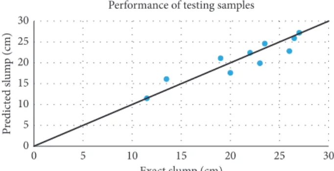
SPNN(7-6-1). The complete offline training process took 31 cycles. The E and R2were 0.0079527 and 0.93996, respectively. After the SPNN was trained on the 285 training samples, it was tested to observe how accurately it would predict slump of other samples. Table 10 and Figure 11 summarize the results of these tests, indicating that the SPNN can satisfactorily predict the slump in all 10 testing samples.
4.2.2. Sensitivity Analysis of the SPNN. Figure 12 shows the
distribution of slump and SP for the training samples of the SPNN. It shows that slump increases with an increase in the amount of SP in the concrete mixture. Slump is proportional to SP, and the slope of the fitted simple regression line is 0.6246. Figure 13 shows the distribution of SP and the first-order partial derivative of slump with respect to SP for the SPNN training samples. The mean of the first-order partial derivative of slump with respect to SP for the training samples of the SPNN is −0.146. The negative mean value of the first-order partial derivative of slump with respect to SP indicates negative correlation between slump and SP, which is inconsistent with the positive slope value of the fitted simple regression line in Figure 12. The reason may be that SP is a material with larger variance, and the properties of different brands of SP are different.
4.3. Experimental Program. Experimental specimens were
also made in the laboratory to study the prediction accuracy of the CSPNN and SPNN in terms of pozzolanic concrete conforming to the ACI concrete mixture code. Twelve concrete mixtures (listed in Table 11) were generated ran-domly by computer program according to the concrete mixture in ACI code. Four experimental specimens were made for each concrete mixture.
4.3.1. Prediction of Compressive Strength. Figure 14 shows
a comparison of exact compressive strength to CSPNN-y = 0.087 0.00 0.05 0.10 0.15 0.20 0.25 0 5 10 15 20 25 30 The f ir st-o rder p ar tia l der iva ti ve o f co m p res si ve str en gt h wi th r esp ec t t o S P SP (kg/m3)
Figure 10: Distribution of SP and the first-order partial derivative of compressive strength with respect to SP for the training samples of the CSPNN. 0 5 10 15 20 25 30 0 5 10 15 20 25 30 Pr edic te d sl um p (cm) Exact slump (cm) Performance of testing samples
Figure 11: Performance of the 10 testing slump samples.
y = 0.6246x + 19.345 0 5 10 15 20 25 30 35 40 0 5 10 15 20 25 30 Sl um p (cm) SP (kg/m3)
Figure 12: Distribution of slump and SP for the training samples of the SPNN.
Table 10: Comparison of exact slump with SPNN-predicted slump for the 10 testing samples.
No. of sample Exact slump (Se) (cm) Predicted slump (Sp) (cm) Se-Sp (cm) 1 23.0 19.9 3.1 2 20.0 17.6 2.4 3 23.5 24.6 −1.1 4 27.0 27.2 −0.2 5 13.5 16.1 −2.6 6 11.5 11.5 0.0 7 22.0 22.4 −0.4 8 26.5 25.9 0.6 9 26.0 22.8 3.2 10 19.0 21.1 −2.1 y = –0.146 –0.45 –0.40 –0.35 –0.30 –0.25 –0.20 –0.15 –0.10 –0.05 0.00 0.00 5.00 10.00 15.00 20.00 25.00 30.00 The f ir st-o rder p ar tia l der iva tiv e o f sl um p wi th r esp ec t t o S P SP (kg/m3)
Figure 13: Distribution of SP and the first-order partial derivative of slump with respect to SP for the training samples of the SPNN.
T able 11: T welve experimental concrete mixtures and their exact and predicted compressive strength and slump. No. of concrete mix Water (kg/m 3 ) Cement (kg/m 3 ) Fly ash (kg/m 3 ) GGBFS (kg/m 3 ) CA (kg/m 3 ) FA (kg/m 3 ) SP (kg/m 3 ) Exact compressive strength (f ′c,e ) (MPa) Predicted compressive strength (f ′c,CSPNN ) (MPa) f ′c,e -f ′c,CSPNN (MPa) Exact slump (Se ) (cm) Predicted slump (SSPNN ) (cm) Se − SSPNN (cm) 1 194 223 72 76 1040 669 0.74 44. 10 34.32 9.77 19.0 19.0 0.0 2 184 244 19 105 1104 649 0.79 47.99 32.26 15.73 20.0 18.5 1.5 3 187 194 22 17 1 1072 650 0.8 1 49.75 34.85 14.90 20.0 19.0 1.0 4 189 272 14 12 1 1040 670 0.70 52.87 35.60 17.27 20.0 19.2 0.8 5 19 1 346 41 38 1136 549 0.73 46.70 45.96 0.74 20.0 16.9 3. 1 6 189 26 1 57 93 1072 619 0.88 47.06 39.04 8.02 20.0 18.7 1.3 7 204 33 1 54 99 1136 457 0.77 54.52 54.55 -0.03 18.0 14. 1 3.9 8 19 1 280 46 12 1 1104 555 0.68 47.6 1 50. 16 -2.55 19.5 17.2 2.3 9 210 300 51 13 1 1040 535 0.54 46.06 52.05 -5.99 20.5 16.7 3.8 10 207 430 61 20 960 604 0.76 54.30 40.08 14.22 21.0 19. 1 1.9 11 190 329 52 112 1104 516 0.87 54.98 55.07 -0.09 19.0 17.2 1.8 12 208 35 1 12 1 52 960 554 0.72 55. 13 40.9 1 14.22 21.5 14. 1 7.4
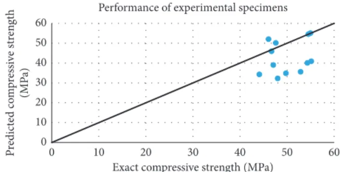
predicted compressive strength for the 12 experimental concrete mixtures. The compressive strength of each con-crete mixture is the average compressive strength of the four specimens for each concrete mixture. Most exact compressive strength values are larger than the CSPNN-predicted com-pressive strength values. Possible reasons may be that (1) coarse aggregates were crushed by machine; thus, the edges of coarse aggregates are sharp, producing a good interlocking effect which increases compressive strength or that (2) ex-perimental specimens were kept submerged in lime water, and the fine weather and relative humidity was sufficient during the curing period to cause the concrete hydration to occur more quickly such that the late compressive strength was reached early. Although some predicted errors of com-pressive strength are large, it is still acceptable.
4.3.2. Prediction of Slump. Figure 15 shows a comparison of
exact slump to SPNN-predicted slump for the 12 experimental concrete mixtures. The slump of each concrete mix is the average slump of the four specimens for each concrete mixture. Most predicted errors for slump are within the al-lowable data range for width of slump (3.8 cm), with only one being extreme (7.4 cm). The predicted error of slump may be mainly caused by SP, since SP is a material with larger variance and the properties of different brands of SP are different. Notably, CSPNN and SPNN were trained using experimental data of pozzolanic concrete mixture proportioning collected from the literature. It is believed that predicted error of compressive strength and slump can be largely decreased if a sufficient number of experimental specimens could be made and used for training of CSPNN and SPNN.
The trained and tested CSPNN and SPNN represent accurate models for compressive strength and slump, re-spectively, and they were used to predict compressive strength and slump of experimental and numerical data. Among 1500 experimental and numerical data, 278 data satisfy Equation (14) and they were kept in the dataset.
4.4. Classification of Pozzolanic Concrete Mixture Proportioning. After establishing the dataset of pozzolanic
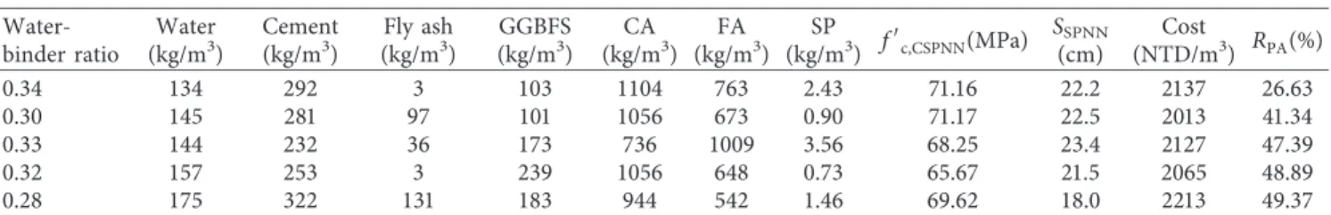
concrete mixture proportioning, it was classified further according to compressive strength, pozzolanic admixture re-placement rate, and cost of concrete. Tables 12 and 13 give some of the results. Table 12 lists concrete mixture pro-portioning samples for compressive strength � 210 kgf/cm2and cost ≤2000 NTD/m3. Table 13 lists concrete mixture pro-portioning samples for compressive strength � 700 kgf/cm2 and 2000 NTD/m3≤ cost ≤ 2250 NTD/m3. Engineers can uti-lize the classified dataset to easily predict mix proportioning (solution) from required compressive strength of concrete, pozzolanic admixture replacement rate, and cost of concrete.
5. Conclusions
This study develops a two-step computer-aided approach for pozzolanic concrete mix design. The first step is to establish a dataset of pozzolanic concrete mixture proportioning that conforms to ACI code. In this step, ANNs are employed to
establish the prediction models of compressive strength and slump of concrete. The second step is to classify the dataset of pozzolanic concrete mixture proportioning. A classification method is utilized to categorize the dataset into 360 classes based on compressive strength of concrete, pozzolanic ad-mixture replacement rate, and material cost. The following important conclusions are drawn from the results:
(1) The CSPNN and SPNN were trained using a portion of collected experimental data. After training, the CSPNN and SPNN were tested using the rest of collected experimental data and data of experimental specimens made in our laboratory for twelve different mixtures. Results prove that CSPNN and SPNN can satisfactorily predict compressive strength and slump, respectively, from respective amounts of water, ce-ment, ground granulated blast furnace slag, fly ash, coarse aggregate, fine aggregate, and superplasticizer. (2) Sensitivity analysis of the ANN can be used to explore the cause and effect relationship between network input and output. Therefore, sensitivity analysis of the CSPNN and SPNN, respectively, can be used to evaluate the effect of various concrete mix constitu-ents (water, cement, ground granulated blast furnace slag, fly ash, coarse aggregate, fine aggregate, and superplasticizer) on the compressive strength and slump of concrete. 0 10 20 30 40 50 60 0 10 20 30 40 50 60 Pr edic te d co m pr es si ve str en gt h (MP a)
Exact compressive strength (MPa) Performance of experimental specimens
Figure 14: Comparison of exact compressive strength with CSPNN-predicted compressive strength for the 12 experimental concrete mixtures. 0 5 10 15 20 25 0 5 10 15 20 25 Pr edic te d sl um p (cm) Exact slump (cm)
Performance of experimental specimens
Figure 15: Comparison of exact slump with SPNN-predicted slump for the 12 experimental concrete mixtures.
(3) The distribution of slump and SP for the training samples of the SPNN shows that slump increases with an increase in the amount of SP in the concrete mixture. Slump is proportional to SP, and the slope of the fitted simple regression line is a positive value (0.6246). However, the mean of the first-order partial derivative of slump with respect to SP for the training samples of the SPNN is a negative value (−0.146). The negative mean value of the first-order partial de-rivative of slump with respect to SP indicates neg-ative correlation between slump and SP, which is inconsistent with the positive slope value of the fitted simple regression line. The reason for this may be that SP is a material with larger variance and the properties of different brands of SP are different. (4) To construct a dataset of pozzolanic concrete
mix-ture proportioning which is practical and convenient for engineering applications, it is classified further. Engineers can utilize the classified dataset to easily predict mix proportioning from required compres-sive strength of concrete, pozzolanic admixture re-placement rate, and the necessary cost of concrete.
Abbreviations
AAN: Artificial neural network
ACI: American Concrete Institute
BFGS method: Broyden–Fletcher–Goldfarb–Shanno
method
BP network: Back-propagation network
CA: Coarse aggregate
classp: The class the pth instance in the
database belongs to
CSPNN: Compressive strength prediction neural
network
d: Search direction
D1ki: The first-order partial derivative of the
kth output with respect to ith input
D1ki: The mean of D1
ki
dpk: The desired output of the kth output
node for the pth instance
dis(a, b): The Euclidean distance between two
vectors (points) a and b
disp,i: The Euclidean distance between the
vector associate to the pth instance in the dataset
E: Mean square error
f: The activation function
FA: Fine aggregate
fc′: Compressive strength
fc,CSPNN′ : Compressive strength predicted by CSPNN
fc,i′: Mean (designed) compressive strength
of the ith class
fc,p′ : Compressive strength of the pth
instance in the dataset
GGBFS: Ground granulated blast furnace slag
H: The inverse Hessian matrix
Hnj: The output of the jth node in the nth
hidden layer L-BFGS learning
algorithm:
Limited memory
Broyden–Fletcher–Goldfarb–Shanno
Oi: The output of ith node
opk: The calculated output of the kth output
node for the pth instance
P: The number of instances in the training
set
PA: Pozzolanic admixtures
R2: The absolute fraction of variance
RPA: Admixture replacement rate
S: Slump
Si: The mean (designed) slump of the ith
class
Sp: The slump of the pth instance in the
dataset
SSPNN: Slump predicted by SPNN
SP: Superplasticizer
SPNN: Slump prediction neural network
Table 12: Concrete mixture proportioning samples for compressive strength � 210 kg/cm2and cost ≤2000 NTD/m3.
Water-binder ratio Water (kg/m3) Cement (kg/m3) Fly ash (kg/m3) GGBFS (kg/m3) CA (kg/m3) FA (kg/m3) SP (kg/m3) f′c,CSPNN(MPa) SSPNN (cm) Cost (NTD/m3) RPA(%) 0.55 199 337 20 6 704 991 0.74 23.80 20.4 1952 7.16 0.55 192 244 65 41 1024 703 2.26 23.45 23.0 1858 30.29 0.48 177 221 39 106 1136 629 3.58 21.55 22.9 1971 39.62 0.52 186 195 72 92 1056 671 2.67 23.87 23.3 1826 45.68
Table 13: Concrete mixture proportioning samples for compressive strength � 700 kg/cm2and 2000 NTD/m3< cost ≤ 2250 NTD/m3.
Water-binder ratio Water (kg/m3) Cement (kg/m3) Fly ash (kg/m3) GGBFS (kg/m3) CA (kg/m3) FA (kg/m3) SP (kg/m3) f′c,CSPNN(MPa) SSPNN (cm) Cost (NTD/m3) RPA(%) 0.34 134 292 3 103 1104 763 2.43 71.16 22.2 2137 26.63 0.30 145 281 97 101 1056 673 0.90 71.17 22.5 2013 41.34 0.33 144 232 36 173 736 1009 3.56 68.25 23.4 2127 47.39 0.32 157 253 3 239 1056 648 0.73 65.67 21.5 2065 48.89 0.28 175 322 131 183 944 542 1.46 69.62 18.0 2213 49.37
SSE: Sum of the squares error
Whnj,ok: The weight associated with the jth node in the nth hidden layer to the kth node in the output layer
Whnjn,ok: The weight associated with the jnth node in the nth hidden layer to the kth node in the output layer
Wij: The weight associated with the ith node
in the preceding layer to the jth node in the current layer
Wxi,h1j1: The weight associated with the ith node in the input layer to the j1th node in the first hidden layer
θj: The threshold value of node j in the
current layer
θok: The threshold value of the kth node in
the output layer
η: Learning ratio
α: Step length.
Data Availability
The data used to support the findings of this study are available from the corresponding author upon request.
Conflicts of Interest
The authors declare that they have no conflicts of interest.
References
[1] N. Bouzoubaa, B. Fournier, V. M. Malhotra, and D. Golden, “Mechanical properties and durability of concrete made with high volume fly ash blended cement produced in cement plant,” ACI Materials Journal, vol. 99, no. 6, pp. 560–567, 2002.
[2] M. Mazloom, A. A. Ramezanianpour, and J. J. Brooks, “Effect of silica fume on mechanical properties of high strength concrete,” Cement and Concrete Composites, vol. 26, no. 4, pp. 347–357, 2004.
[3] K. Tan and X. Pu, “Strengthening effects of finely ground fly ash, granulated blast furnace slag, and their combination,” Cement and Concrete Research, vol. 28, no. 12, pp. 1819–1825, 1998.
[4] C. Ozyildirum and W. J. Halstead, “Improved concrete quality with combination of silica fume and fly ash,” ACI Materials Journal, vol. 91, no. 6, pp. 587–594, 1994.
[5] I. Papayianni, G. Tsohos, N. Oikonomou, and P. Mavria, “Influence of superplasticizer type and mix design parameters on the performance of them in concrete mixtures,” Cement and Concrete Composites, vol. 27, no. 2, pp. 217–222, 2005. [6] D. A. Abrams, Design of concrete mixtures. Bulletin No. 1,
Structural Materials Laboratory, Lewis Institute, Chicago, IL, USA, 1918.
[7] S. Popovics, “Analysis of concrete strength versus water-cement ratio relationship,” ACI Materials Journal, vol. 87, no. 5, pp. 517–529, 1990.
[8] F. De Larrard and M. Buil, “Granularit´e et compacit´e dans les mat´eriaux de g´enie civil,” Materials and Structures, vol. 20, no. 2, pp. 117–126, 1987.
[9] H. Adeli and S. L. Hung, Machine Learning: Neural Networks, Genetic Algorithms, and Fuzzy Systems, Wiley, New York, NY, USA, 1995.
[10] J. Suykens, J. Vandewalle, and J. De Moor, Artificial Neural Networks for Modeling and Control of Non-Linear Systems, Kluwer Academic Publishers, Boston, MA, USA, 1996. [11] D. E. Rumelhart, G. E. Hinton, and R. J. Williams, “Learning
international representation by error propagation,” in Parallel Distributed Processing, D. E. Rumelhart, J. L. McClelland, and The PDP Research Group, Eds., pp. 318–362, The MIT Press, Cambridge, MA, USA, 1986.
[12] I. C. Yeh, “Analysis of strength of concrete using design of experiments and neural networks,” Journal of Materials in Civil Engineering, vol. 18, no. 4, pp. 597–604, 2006. [13] I. C. Yeh, “Modeling of strength of high-performance
con-crete using artificial neural networks,” Cement and Concon-crete Research, vol. 28, no. 12, pp. 1797–1808, 1998.
[14] J. Kasperkiewics, J. Racz, and A. Dubrawski, “HPC strength prediction using ANN,” Journal of Computing in Civil En-gineering, vol. 9, no. 4, pp. 279–284, 1995.
[15] S. C. Lee, “Prediction of concrete strength using artificial neural networks,” Engineering Structures, vol. 25, no. 7, pp. 849–857, 2003.
[16] J. Bai, S. Wild, J. A. Ware, and B. B. Sabir, “Using neural networks to predict workability of concrete incorporating metakaolin and fly ash,” Advances in Engineering Software, vol. 34, no. 11-12, pp. 663–669, 2003.
[17] Z. H. Duan, S. C. Kou, and C. S. Poon, “Prediction of compressive strength of recycled aggregate concrete using artificial neural networks,” Construction and Building Mate-rials, vol. 40, pp. 1200–1206, 2013.
[18] G. H. Ni and J. Z. Wang, “Prediction of compressive strength of concrete by neural networks,” Cement and Concrete Re-search, vol. 30, no. 8, pp. 1245–1250, 2000.
[19] S. L. Hung and Y. L. Lin, “Application of an L-BFGS neural network learning algorithm in engineering analysis and de-sign,” in Second National Conference on Structural Engineering, pp. 221–230, Chinese Society of Structural En-gineering, Nantou, Taiwan, 1994.
[20] J. Nocedal, “Updating quasi-Newton matrix with limited storage,” Mathematics of Computation, vol. 35, no. 151, p. 773, 1980.
[21] T. F. Coleman and Y. Li, Large-Scale Numerical Optimization, Society for Industrial and Applied Mathematics, Philadelphia, PA, USA, 1990.
[22] G. Cybenko, “Approximations by superpositions of a sig-moidal function,” Mathematics of Control, Signals, and Sys-tems, vol. 2, no. 4, pp. 303–314, 1989.
[23] K. Funahashai, “On the approximate realization of contin-uous mappings by neural networks,” Neural Networks, vol. 2, no. 3, pp. 183–192, 1989.
[24] S. L. Hung and C. Y. Kao, “Structural damage detection using the optimal weights of the approximating artificial neural networks,” Earthquake Engineering and Structural Dynamics, vol. 31, no. 2, pp. 217–234, 2002.
[25] C. Y. Kao and S. L. Hung, “Detection of structural damage via free vibration responses generated by approximating artificial neural networks,” Computers and Structures, vol. 81, no. 29, pp. 2631–2644, 2003.
[26] I. C. Yeh and H. B. Zhang, “Comparisons of mixture design of experiments for high performance concrete,” Journal of Technology, vol. 22, pp. 179–185, 2007.
[27] A. S. Cheng, “Research on the microstructure and strength prediction of pozzolanic concrete,” Dissertation, National Chung Hsing University, 2011.
[28] M. Nehdi, M. Pardhan, and S. Koshowski, “Durability of self-consolidating concrete incorporating high-volume re-placement composite cements,” Cement and Concrete Re-search, vol. 34, no. 11, pp. 2103–2112, 2004.
[29] M. A. Megat Johari, J. J. Brooks, S. Kabir, and P. Rivard, “Influence of supplementary cementitious materials on en-gineering properties of high strength concrete,” Construction and Building Materials, vol. 25, no. 5, pp. 2639–2648, 2011. [30] N. Su, K. C. Hsu, and H. W. Chai, “A simple mix design method for self-compacting concrete,” Cement and Concrete Research, vol. 31, no. 12, pp. 1799–1807, 2001.
[31] E. G¨uneyisi, M. Gesoglu, and E. ¨Ozbay, “Evaluating and
forecasting the initial and final setting times of self-compacting concretes containing mineral admixtures by neural network,” Materials and Structures, vol. 42, no. 4, pp. 469–484, 2009.
[32] R. Siddique, “Properties of self-compacting concrete con-taining class F fly ash,” Materials and Design, vol. 32, no. 3, pp. 1501–1507, 2011.
[33] A. Oner, S. Akyuz, and R. Yildiz, “An experimental study on strength development of concrete containing fly ash and optimum usage of fly ash in concrete,” Cement and Concrete Research, vol. 35, no. 6, pp. 1165–1171, 2005.
[34] R. Siddique, “Performance characteristics of high-volume class F fly ash concrete,” Cement and Concrete Research, vol. 34, no. 3, pp. 487–493, 2004.
[35] G. Li and X. Zhao, “Properties of concrete incorporating fly ash and ground granulated blast-furnace slag,” Cement and Concrete Composites, vol. 25, no. 3, pp. 293–299, 2003. [36] G. Li, “Properties of high-volume fly ash concrete
in-corporating nano-SiO2,” Cement and Concrete Research,
vol. 34, no. 6, pp. 1043–1049, 2004.
[37] A. A. Ramezanianpour and V. M. Malhotra, “Effect of curing on the compressive strength, resistance to chloride ion penetration and porosity of concretes incorporating slag, fly ash or silica fume,” Cement and Concrete Composites, vol. 17, no. 2, pp. 125–133, 1995.
[38] M. C. Li, “A study on rational mix proportion and vibra-tion characteristics of high flowing concrete,” Dissertavibra-tion, National Taiwan University, 2010.
[39] S. H. Kosmatka, B. Kerkhoff, and W. C. Panarese, Design and Control of Concrete Mixtures, Engineering Bulletin; 001, Portland Cement Association, Skokie, IL, USA, 14th edition, 2002.
[40] Public Construction Commission, “Chapter 03050: general requirements of concrete basic materials and construction,” in Construction Outline Code for Public Construction, Public Construction Commission, Taipei, Taiwan, 2010.
[41] A. C. Rencher, Methods of Multivariate Analysis, Wiley, New York, NY, USA, 2003.
International Journal of
Aerospace
Engineering
Hindawi www.hindawi.com Volume 2018Robotics
Journal of Hindawi www.hindawi.com Volume 2018 Hindawi www.hindawi.com Volume 2018Active and Passive Electronic Components VLSI Design Hindawi www.hindawi.com Volume 2018 Hindawi www.hindawi.com Volume 2018
Shock and Vibration
Hindawi
www.hindawi.com Volume 2018
Civil Engineering
Advances inAcoustics and VibrationAdvances in Hindawi
www.hindawi.com Volume 2018
Hindawi
www.hindawi.com Volume 2018
Electrical and Computer Engineering Journal of Advances in OptoElectronics Hindawi www.hindawi.com Volume 2018
Hindawi Publishing Corporation
http://www.hindawi.com Volume 2013 Hindawi www.hindawi.com
The Scientific
World Journal
Volume 2018 Control Science and Engineering Journal of Hindawi www.hindawi.com Volume 2018 Hindawi www.hindawi.com Journal ofEngineering
Volume 2018Sensors
Journal of Hindawi www.hindawi.com Volume 2018 Machinery Hindawi www.hindawi.com Volume 2018 Modelling & Simulation in Engineering Hindawi www.hindawi.com Volume 2018 Hindawi www.hindawi.com Volume 2018 Chemical EngineeringInternational Journal of Antennas and
Propagation International Journal of Hindawi www.hindawi.com Volume 2018 Hindawi www.hindawi.com Volume 2018 Navigation and Observation International Journal of Hindawi www.hindawi.com Volume 2018