DESIGN OF SPACE-OPTIMAL REGULAR ARRAYS FOR ALGORITHMS WITH LINEAR SCHEDULES

(1)

IEEE TRANSACTIONS ON COMPUTERS, VOL. 44, NO. 5, MAY 1995 ₆₈₃

Design of Space-Optimal Regular Arrays

for Algorithms with Linear Schedules

Jong-Chuang

Tsay

and Pen-Yuang Chang

Abstract-The problem of designing space-optimal 2D regular arrays for N x N x N cubical mesh algorithms with linear schedule ai

+

bj

+

ck, 1 I a I b 5 c, and N = nc, is studied. Three novel nonlin- ear processor allocation methods, each of which works by combin- ing a partitioning technique (gcd-partition) with different nonlinear processor allocation procedures (traces), are proposed to handle different cases. In cases where a

+

b 5 c, which are dealt with by the first processor allocation method, space-optimal designs can always be obtained in which the number of processing elements is equal to

$

.

For other cases where a

+

b > c and either a = b and b = c, two other optimal processor allocation methods are proposed. Besides, the closed form expressions for the optimal number of processing elements are derived for these cases.

Index Items-Algorithm mapping, data dependency, linear schedule, matrix multiplication, optimizing compiler, space- optimal, systolic array.

I. INTRODUCTION

EGULAR arrays, or systolic arrays [l], 123, have been

R

proposed for over a decade. They are special purpose parallel devices composed of several processing elements (PES) whose interconnections have the properties of regularity and locality. Because of these properties, regular architectures are very suitable for VLSI implementation.

The procedure for synthesizing regular arrays from systems of recurrence equations, or nested loops, has two major steps. The first one is regularization [3], [4], [5], or uniformization [6], which includes variable full indexing [7] (defining all variables on the same index dimension only once); broadcast removing [8] (replacing broadcast vectors with pipeline vectors); reindexing [9] (re-routing pipeline vectors so that they are oriented in the same direction); and so on [lo], [ l l ] , [12]. After regularization, the original system of recurrencc equations is transformed into an equivalent system of uniform recurrence equations

(SURE)

[ 131 or a regular iterative algorithm (RIA) [ 141. A dependence

graph (DG) is a graphical representation of such an algorithm, in

which each node corresponds to an index vector and each link represents a dependence vector between two nodes. A depend-

ence matrix D is the collection of all dependence vectors in an

algorithm; each column in D is a dependence vector. The second

Manuscript received Feb. 17, 1993; revised Apr. 1, 1994.

The authors are with the Institute of Computer Science and Information Engineering, College of Engineering, National Chiao Tung University, Hsinchu, Taiwan 30050, Republic of China; e-mail jctsayOcsunix.csie.nctu. edu.tw.

IEEECS Log Number C95022.

step is to find the spacetime mapping transformation matrix

T =

[

yTT]

[ 131, [ 141, [ 151, [ 161 with a valid linear schedule vec- tor

nT

and a compatible processor allocation matrix

nT

for an SURE. A schedule is valid if the precedence constraints imposed by an SURE are satisfied and a processor allocation is compati- ble with its schedule if two different computations are not executed on the same PE at the same time.

In the past, most researchers focused their efforts on regularization, and the first half of spacetime mapping, the time mapping [13], [14], [15], [17], [18], [19]. In particular, the problem of how to find an optimal linear schedule for an SURE has attracted special interest [20]. Only recently has its counterpart problem- that of how to design space-optimal regular arrays in which the number of PES is minimal for an SURE executed by a given linear schedule-been studied in the literature [21], [22], [23], [24], [25], [26], [27], [28]. Studies of this latter problem fall into

three categories. The first class includes 1211, [22], [23], [241, [25], in which the following method is adopted: first, from the given DG and linear schedule, a set

’?

of nodes is found such that all nodes in the set are scheduled to be executed at the same time and the set size lvl is maximal. We call such a set a maxi- mum concurrent ser with respect to the given linear schedule.

Second, spacetime mapping is applied to assign the nodes of the DG to PES. Any PE which has not been assigned to execute a node in ?/is piled to a PE which executes a node in ?land has disjoined activation time intervals. This method can indeed be used to design space-optimal regular arrays. However, it has two drawbacks. The first is that finding a maximum concurrent set with respect to a linear schedule

n(l)

= ai

+

bj

+

ck is not an easy task, i.e., the nodes must be represented in a closed form expression by the parameters a, b, c, and N , where N is the problem size parameter. Thus this method designs space-optimal regular arrays case by case. Second, piling PES results in spiral links and increases irregularity for the resulting arrays.

The second class of methods for designing space-optimal arrays [25], [26], [27] deals with this problem by grouping llTq PES into a single one, where qT is the projection vector with respect to the space mapping matrix ST(STq = 0). Thus the resulting array has a 100% pipelining rate. The advantages of this method are that it is not necessary to find a maximum concurrent set, the resulting array does not have spiral links, and the method is applicable to all SUREs. However, this method cannot guarantee that the design is space-optimal, because a 100% pipelining rate in the array does not imply space- optimality. The regular array for matrix multiplication is a

(2)

684 IEEE TRANSACTIONS ON COMPUTERS, VOL. 44, NO. 5 . MAY 1995

good example; it has FITq = [ 1 1 11 [0 0 1IT = 1 but is not space-optimal.

In the third class [28], an upper bound on the length of the optimal projection vector is developed and an enumerative search procedure for finding the optimal projection vector is provided. However, this approach does not provide space- optimal designs in a general way, because only linear processor allocation is considered.

For the problem of designing space-optimal regular arrays, two interesting questions we want to investigate are: first, how many PES are needed to design a regular array for a given

N x N x N DG with a linear schedule

n(l)

= ai

+

bj

+

ck. For

simplicity, the problem domain in this paper is restricted to a cubical mesh. Second, how to design a regular array which is not only space-optimal but also is locally connected, provides balanced loads, and allows for simple control. In the following, several nonlinear processor allocation procedures will be proposed to design space-optimal regular arrays for different cases. The linear schedule

n(l)

= ai

+

bj

+

ck with 1 I a I b I c is considered. It is easy to see that an algorithm with an

arbitrary linear schedule, say FI’(Z) = a’i

+

b’j

+

c’k, where a‘, b’, and c‘ are all non-zero integers, can be transformed to an

equivalent one with

n(Z)

= ai

+

bj

+

ck and 1 I a I b 5 c by

applying permutation transformations [29]. Therefore, without loss of generality, we assume that 1 I a 5 b 5 c. In addition,

for simplicity, we also assume that N = nc in the following

descriptions. Furthermore, an algorithm with an arbitrary uni- form affine schedule [30]

n,(l)

= ai

+

bj

+

ck

+

u can also be transformed to an equivalent one with a linear schedule by

timespace mapping or dimension extension [3 I].

In Section 11, some important definitions are given. In Section 111, the gcd-partition method and the first processor allocation procedure will be introduced to design space-optimal regular arrays for the case of a

+

b 5 c. It is proven that in such a case

$

is the minimum number of PES required or the size of a maximum concurrent set for the given linear schedule. A space- optimal regular array for transitive closure and algebraic path problem will be given to illustrate our method. In Section VI, the other two optimal processor allocation procedures are developed to handle the cases of a = b and b = c, respectively, when a

+

b >

c, and the closed form expressions for the size of a maximum

concurrent set will also be given for both cases. A new space- optimal regular array for matrix multiplication will also be given. Finally, our concluding remarks are presented in Section V.

11. PRELIMINARIES

The variables used in this paper are all integral numbers. Each index vector in the computation domain Y is denoted by I =

[ i j kIT, where 1 I i, j , k

<

N . The linear schedule

n(Z)

= ai

+

bj

+

ck with 1 I a I b I c is a normalized one, i.e., gcd(a, b, c) = 1.

DEFINITION 2.1. [locally connected]. A regular array is said to be locally connected iff any communication link between two PES has a displacement vector independent of the size of the problem.

DEFINITION 2.2. [space-optimal]. A regular array is said to be space-optimal with respect to a given linear schedule for an

SURE lflthe number of PES used (denoted by PEused) is equal to the size of a maximum concurrent set, or the mini- mum number of PES required (PEmin), for the given linear schedule.

Clearly, for a given linear schedule, if PEUsd < PE,,, then two different computations will be executed on the same PE at the same time.

DEFINITION 2.3. [time-tag]. A time-tag v = ai

+

bj

+

ck (or, in indexed notation, u f J ) is a positive integral number assigned to each node or index vector [ i j kIT in the com- putation domain ‘I’ of an SURE to represent the execution time of the index vector with respect to the linear schedule vector [a b elT.

DEFINITION 2.4. [modulo set]. Given a positive integer r, 0 I r <

c, a modulo set Nr) is a set of nodes of ’I’ such that each node of N r ) has an assigned time-tag v satisfying mod(v, c) = r, where mod(a, b) denotes the remainder of a divided by b.

A multiset [32]

M

is a collection of not necessarily distinct elements. It may be thought of as a set in which each element, say v, has an associated positive integer, its multiplicity Cv(M),

to represent the number of vs in

M.

For example,

M

=

{ 1, 1, 2, 2, 2, 2, 3 ) is a multiset, where C1(@ = 2,

Cz(M) = 4, and C3(M) = 1. We use the multiset W to denote the collection of the time-tags of all the index vectors in Y for an SURE.

DEFINITION 2.5. [partition]. A possible partition

P

of W is written as {VI, V2,

...

V,,,), where each VI in

P

is a set of time-tags and the partition size P I = m.

DEFINITION 2.6. [optimal partition]. An optimal partition is a partition such that its partition size is minimal with respect to all possible partitions of W.

EXAMPLE 2.1. This example demonstrates the concept of an optimal partition: Let W = (1, 2, 2, 3, 3, 3, 4, 4, 5 ) . A pos- sible partition

PI

= ( V I , V2, Vj, V 4 ) = { ( I , 2, 3 } , (2, 3 } ,

( 4 } , ( 3 , 4, 5 ) ) . However, PI is not optimal, because it is easy to find an optimal partition

P,

= ( V I , Vz, V j } = ( { I , 2, 3 } , {2, 3, 4 } , (3, 4, 5 ) ) such that IP,l <

lPIl.

Of course, there m y exist several optimal partitions, but at least one optimal partition always exists.

The following lemma states a useful property of optimal partitions.

LEMMA 2.1. A partition

P

is optimal iff there exists a time-tag

PROOF. For any partition, we have I

P

I 2 max,, wC,( W).

v E V I for all VI E

P.

[If part] If there exists a time-tag v E VI for all VI E

P,

we have

lp( =

c,,(w)

= max,,,&,,(W). Then lp( is minimal with respect to all possible partitions of W, i.e., the partition

P

is optimal. [Only if part] It is obvious that if lp( is minimal with respect to all possible partitions of W, then lp( = max,,&(W) 3 Cv(W);

this implies that there exists a time-tag v E VI for all VI E

P.

u

The following definitions are important because they are the basis for finding optimal partitions systematically.

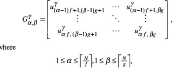
DEFINITION 2.7 [segment, segment domain]. A segment is de- fined as an f x g matrix

(3)

TSAY A N D CHANG: DESIGN OF SPACE-OPTIMAL REGULAR ARRAYS FOR ALGORITHMS WITH LINEAR SCHEDULES 685

where

and y = k (see Fig. 1). The segment domain 0 is constructed by the set of segments.

k

f-.i

i

Fig. 1. The concept of a segment.

We use the notation u: E G,Y,p to represent that ut is an element of the segment G&. The value of a pair of comma- separated integers @, q ) gives the coordinates of the location of the time-tag on the segment. The first number is the vertical coordinate, and the second number is the horizontal coordinate, measured from the top left corner of the segment. We say that two time-tags of different segments have the same (p, q )

location if they are located at the same @, q ) coordinates in their respective coordinate systems.

DEFINITION 2.8 [module, cluster]. A module G,,p is a set of segments and a cluster G is a set of modules.

A time-tag uf, is said to be in module Gsp (denoted by uf,, E G,,p) if E G& and G& E G,,p. Similarly, a time-tag

uf is said to be in cluster G (denoted by ut E G) if u t j E G,,p and G,,p E G. Various grouping methods can be used to construct modules. For example, by simply collecting all segments

G& in the k-direction, the module Gsp = { ..., G& } is constructed. A more complex grouping method is described by the following concept:

DEFINITION 2.9 [trace]. A trace (GL:.pl, 0) is a module consisting

of the set of segments on a directed path that begins from

where all segments of a trace belong to the segment domain 0.

DEFINKION 2.10 [size]. The size of a segment, module, and cluster, denoted by lG&I, I, and lGl represent the number of time-tags, segments, and modules in them, respectively.

DEFINITION 2.11 [modulo-s segment]. A segment G,Y,p is said modulo-s iff for every time-tag v E G,Y,p there does not exist another time-tag V I E G& such that mod(v, s) = mod(v1, s), where s > 0.

DEFINITION 2.12 [isomorphic segments]. Two f x g segments

G&, G&, are said to be isomorphic i y f o r any two time- tags v E G,Y,p, v1 E GL;,pl,

if

they have the same (p, q) loca- tion, then (v, l G,Y,p I) = mod(vl, l G&, l).

DEFINITION 2.13 lfree segment]. A segment is said to befree iff it has not yet been allocated to a module, and the notation free(@) represents the set of free segments in the segment do-

main 0.

DEFINITION 2.14 [minimal index vector, minimal segment]. An index vector I = [i j kIT is said to be minimal with respect to a domain $there does not exist another 11 = [il j l kllT in this domain such that (kl < k) v ((kl = k) A (jl < j ) ) v ((kl =

k) A ( j l = j ) A (il < i)). A segment G& is said to be minimal with respect to a set of segments

r,

denoted by G& = m i n { r } ,

iff

there is a time-tag in G& E

r

assigned to the

minimal index vector I = [i j kIT.

DEFINRION 2.15 [elementary module]. A module G,,p is said to be elementary irfor any two time-tags V I , v2 E G,,p, V I f V I .

With this definition, it is obvious that an elementary module is a set of time-tags. The concept of an elementary module is very important. In our processor allocation procedures, each module is allocated to one PE. An elementary module ensures that no two different computations are scheduled to be executed on the same PE at the same time, i.e., the processor allocation procedure is compatible with the given schedule. DEFINITION 2.16 [elementary cluster]. A cluster G is said to be

elementary iff every module G,,p E G is elementaly.

said to be optimal iff IGI is minimal. size lPl of an optimal partition for W.

DEFINITION 2.17. [optimal cluster]. An elementary cluster G is

LEMMA 2.2. The size lGl of an optimal cluster is equal to the

PROOF. Under the assumption that every module G,,b E G is elementary, we have lGl 2. max,,&(G). Thus G is an optimal cluster when IGI = max,,GCV(G). From Lemma 2.1 and the observation that the multiset W is equal to the multiset

G, we have lGl = IPI. - 1

(4)

686 IEEE TRANSACTIONS ON C O M P U T E R S , VOL. 44, NO. 5 , MAY 1995

finding an optimal cluster. In the following sections, several procedures for finding an optimal cluster will be introduced. The central concept is to partition every ij-plane of the DG into several segments, to group these segments into several elementary modules, and to keep the number of modules in a cluster to a minimum.

111. PROCESSOR ALLOCATION FOR a

+

b I c

A. Procedure

In this section, a new processor allocation procedure for algorithms with linear schedules is proposed. This procedure guarantees that the derived regular array is space-optimal for an SURE with a linear schedule

n(Z)

= ai

+

bj

+

ck when a

+

b I c. For other situations, although a space-optimal regular ar-

ray cannot always be obtained, our procedure still decreases the number PES used from N2 (if a 2 x 3 linear processor allo- cation matrix is used) to

$.

PROCEDURE 3.1. Given a 3 0 SURE with a linear schedule

n(I) = ai

+

bj

+

ck and a

+

b I c, a space-optimal regular array can always be obtained by partitioning every ij-plane of the DG of the SURE into

x g segments GL,p, where g g = &(a, c ) , 1 I

a

I ?,

gN

1 I p I

N

-, and 1 I y 5 N , g or g x c segments G:,p, where g g = g c d ( b , c ) , l I a r I - - , l I P 5 ~ , a n d l I

N

y l N . g

Then each module (PE) is constructed by collecting the set

0

This method of partitioning is called gcd-partitioning. Us- ing this method, a module is constructed by tracing the set of segments in the k-direction. This method of constructing modules is designated Tracel and can be defined as G,,p =

Tracel(Gk,p, 0) = < Gh,p, G:,p,

...,

G& >. Using the same gcd-partition but different traces to construct modules results in different processor allocation procedures.

EXAMPLE 3.1 [transitive closure and algebraic path problem].

From the DG of transitive closure derived by S.Y. Kung et al. [9] (DG-3 in their paper), the dependence matrix can be written as

of segments in the k-direction.

D =

[I

0 1 - 1

::

0 - 1 , -11

:I

and the corresponding optimal linear schedule is n(1) = i

+

j

+

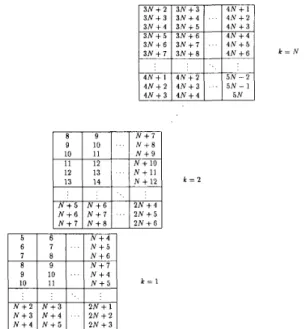
3k. Thus by applying Procedure 3.1, time-tags on ever):

ij-plane can be gcd-partitioned into several 3 x 1 segments,

I 3 N + 2 I 3 N + 3 I I 4 N + 1 I 4 N + 2 4 N + 3 4 N + 3 4 N + 4 5 N N + 10 12 13 N + 1 1 13 14 N + 12 N + 5 N + 6 2 N + 4 N + 6 N + 7 .. 2 N + 5 N + l N + 8 2 N + 6 k = 1 N + 2 N + 3 2 N + 1 N + 3 N + 4 . . 2 N + 2 N + 4 N + 5 2 N + 3 k = 2

Fig. 2(a). The DG of transitive closure and algebraic path problem is gcd- partitioned into several 3 x 1 segments.

Fig. 2(b). Constructing modules by Tracel.

11:

q

i

&2.it.

. . .

Fig. 2(c). The space-optimal regulaf'axky for transitive closure and algebraic

path problem.

Fig. 2(b). A space-optimal regular array with only can be obtained as shown in Fig. 2(c).

PES

as shown in Fig. 2(a). A module (PE} is constructed by collecting segments in the k-direction (Trace,), as shown in

The DG for the algebraic path problem derived by Lewis and Kung [33, Fig. 31 can be reindexed as ( [ i j klT t

(5)

687 TSAY AND CHANG: DESIGN OF SPACE-OPTIMAL REGULAR ARRAYS FOR ALGORITHMS WITH LINEAR SCHEDULES

[i

-

k

+

1

for transitive closure, and the same result can be obtained. E

j - k

+

1 kIT) to construct a DG similar to that

B. Validity

In this section, we want to prove that Procedure 3.1 can derive a locally connected, space-optimal regular array for any SURE with a linear schedule

n(Z)

= ai

+

bj

+

ck and a

+

b 5 c.

LEMMA 3.1. The regular array derived by Procedure 3.1 is locally connected.

PROOF. Because each PE corresponds to a module constructed by collecting the segments in the k-direction, the locally il THEOREM 3.1. Procedure 3. I is compatible with its schedule PROOF. A processor allocation procedure is said to be com- patible with the given schedule iff no two different computations are executed on the same PE at the same time, and that is the central feature of an elementary module. Thus in this proof, first, two properties of segments traced by the gcd-partition in Procedure 3.1 are derived; one is that every segment is modulo-c and the other is that any two segments in a module are isomorphic. With these properties, it can be proved that each module is elementary.

[modulo-c]

gcd(a, c ) = g : According to Procedure 3.1, every ij-plane should be partitioned into several segments. The size of each segment G& is f~ g , where (with h E L )

connected links can always be obtained.

n(Z)

= ai

+

bj

+

ck. GL,p

1

v + b ... v + ( g - l ) b v + a + b ... v + a + ( g - l ) b l v + ( h - l ) a v + ( h - 1)a

+

b ... v + ( h - l ) a + ( g - 1)bJ

If c = 1 then there is only one time-tag in every segment; it is modulo-1. For c > 1 and any two time-tags vl, v2 E G&, the difference between the time-tags is v2

-

v1 = ia +jb, where 1

-

h I i I h - 1 , 1 - g 5 j I g

-

1.

By contradiction, assume that G,Y,p is not a modulo-c segment, Le., there exist two time-tags vl, v2 E G i , p , and

v2 = v1

+

mc such that v2 = v1

+

ia

+

j b = v1

+

mc.

(1) Let a = ga’; then we have iga’

+

j b = mgh.

+

j b = (mh -ia’)g m’g.

a ia

+

j b = mc

(2)

* ” = - j b S

Because m‘ must be an integer, only two cases are possible: If m‘ = 0 then j = 0. Equation (1) can then be re- duced to ia = mc = q x Icm(a, c), where q is an inte-

ger and Icm(a, c ) denotes the least common multi- plier of

a

and c. From this equation, we have lial 2

Icm(a, e). Because 1 - 5 i

<

C

-

1 or lial 5 2 -

a = Icm(a, c ) - a < Icm(a, c), a contradiction occurs. If m’ # 0 then j # 0. We know gcd(a, b, c ) = 1, be- cause the linear schedule

n(Z)

= ai

+

bj

+

ck is a normalized one. If gcd(a, c ) = g = 1, then by 1 - g I

j 5 g - 1, we have j = 0. This is a case which we have explored already. On the other hand, if gcd(a, c ) = g f I , then gcd(b, g ) = 1. From g > ljl, the right-hand side of (2),

$,

cannot be an integer. Thus a contradiction occurs, because the left-hand side of (2), m‘, is an integer.

In both cases there are contradictions. This implies that

G& is a modulo-c segment.

gcd(b, c ) = g : The argument is similar to that for gcd(a, c ) = g .

It has now been shown that every segment derived by Pro- cedure 3.1 (gcd-partition) is modulo-e.

[isomorphic]. Let v1 and v2 be two time-tags which have the same (’p, q ) location about two different segments, say GLtp

and G,‘:p, respectively, in a module. Let the index vector for v1 be [il j l kllT and that for v2 be [il j , k2IT. Then v1 = ail

+

bjl

+

ckl and v2 = ail

+

bjl

+

ck2.

+

~2 - V I = c(k2 - kl). (3)

(4) Because the size of every segment obtained by Procedure 3.1 is c, we have mod(vl, lG&,’pI) = mod(v2, IGL:pI). This shows that every segment in a module derived by Procedure 3.1 is isomorphic to all others.

Since every segment is modulo-c and is isomorphic to all others in the module, it can now be proved that each module is elementary.

[elementary]. Let v1 and v2 (viand v;> be two time-tags with the same (’p, q) location about two different segments, say

GLlp and GLYp, respectively, in a module. Let the index vector for v1 be [il j l kllT and that for v2 be [il j l k2IT.

Then v1 = ail

+

bjl

+

ckl and v2 = ail

+

bj,

+

ck2. Similarly,

let the index vector for v; be [i; j ; k1lT and that for

vi

be [i;

j ; k2IT. Then v; = ai;

+

bj;

+

ckl and

v i

= ai;

+

bj;

+

ck2.

0 <vl, v2>: If two index vectors belong to different seg-

ments in a module but have the same (p, q ) location with respect to their segments, then their time-tags should be different, because (3) is not equal to zero.

0 <v2, vi>: If two index vectors belong to the same seg-

ment, then their time-tags are not the same. Since GL,’p is modulo-c, we have (v2, c ) # mod(& c),

+

v2 f vi.

0 <vl, vi>: If two index vectors belong to different seg-

ments and have different (p, q ) locations, then their time- tags are not the same. The reason is as follows: Because

GLfp is modulo-c, we have mod(v2, c ) # mod(v;, c ) , and from (4), mod(vl, e ) = mod(v2, c),

*

mod(v,, c ) f mod(& c), 3 V I #

vi.

(6)

688 _{IEEE TRANSACTIONS ON COMPUTERS,}_VOL._44,_NO._{5 ,}_{MAY 1995}

No other case.

Because any two index vectors in a module have different time-tags, the module is elementary. Hence every module

0

THEOREM 3.2. The regular array derived by Procedure 3.1 is constructed by Procedure 3.1 is elementary.

space-optimal.

PROOF. To prove that Procedure 3.1 can derive a space- optimal regular array is equivalent to proving that the cluster G derived by Procedure 3.1 is optimal. Lemmas 2.1 and 2.2 tell us that a cluster G is optimal iff every module G,,p

E G is elementary and there exists a time-tag v E Ga,p for all G,,p E G. The former has been shown in Theorem 3.1.

Now we want to prove that there is at least one time-tag v E

G,,p for all G,,p E G if Procedure 3.1 is applied.

Let v2 be the largest time-tag on the (k = 1)-plane with a remainder r when divided by e, i.e.,

v2 = m 2 c + r EGL &y

g ’ c ’

where

g = gcd(b, c) (or G h where g=gcd(a,c)

_r.:.

.

Because every segment derived by Procedure 3.1 is modulo-c, one can find a time-tag V I = mlc

+

r E GL, p, 1 I a ,<: 1 I

p <

F.

The difference between V I and v2 is v2 -

V I = (m2

-

ml)c. 3 m2

-

ml =

-

=

m‘. In addition, the dif-

ference between any two time-tags on the (k = 1)-plane is equal to or less than ( a

+

b)(N

-

l), because the maximum and minimum time-tags on this plane are aN

+

bN

+

c (the

node [N N 1IT) and a

+

b

+

c (the node [ l 1 1IT), respectively. Thus

v 2 - v, ~ ( ( 1 + b ) ( N - 1)

C C

From a

+

b I c, we have

PROOF. The theorem follows directly from Lemma 3.1, Theo-

U

rem 3.1, and Theorem 3.2.

From Procedure 3.1, because the number of time-tags in every segment is c and every module contains N segments, the number of time-tags in each and every module is Ne. Mean- while, because there are N3 time-tags in the computation do- main, the size of the cluster or the number of PES used is

$.

On the other hand, Theorem 3.2 manifests the fact that the regular array is space-optimal, Le., the number of PES used (modules) by Procedure 3.1 is equal to the minimum number of PES required. Thus

$

is just the lower bound of the number of PES required so that no two different computations are executed on the same PE at the same time. Therefore we have the following theorem.

THEOREM 3.4. The minimum number of PES required is

$

f or any SURE with a linear schedule

n(I)

= ai

+

bj

+

ck

and a

+

b I e.

Procedure 3.1 is a simple but useful method of processor allocation for deriving a space-optimal regular array. The array derived is locally connected and regular and provides simple control and a balanced load. However, Procedure 3.1 guarantees that the optimal space is obtained only when the linear schedule

n(l)

= ai

+

bj

+

ck follows the constraint of a

+

b 5 c. The case where a

+

b > c will be discussed in the next section.

VI. PROCESSOR ALLOCATION FOR a

+

b > c

Now let us discuss the more difficult case, a

+

b > e. In this

case, (5) is not always true and a time-tag v may not always be found in every module derived by Procedure 3.1. Thus a space-optimal regular array cannot always be obtained, Le., the difference between PEurpd and PEmi,, is a function of N (problem size parameter). Yet, Procedure 3.1 can still be used to decrease PEused from N2 to

$

when a

+

b > c. For example, given a linear schedule

n(l)

= 2i

+

3j

+

4k and N = 20, the 2 x ( a + b ) ( N

-

1) ( a

+

b ) ( N - 1)

- = N - 1

c u + b

2 segment can be obtained by the gcd-partition of Procedure 3.1; then by Tracel, N segments can be grouped in the

( 5 )

Then 1 5 m’ 5 N - 1, Therefore, if we have the time-tag k-direction to construct a ~ c 3 d u k (PE). Thus we have P E m d =

$

= 100, which is greater than the size of a maximum concurrent set, 96, for the given linear schedule. Nevertheless, when a

+

b > c, a space-optimal regular array can be designed for the special cases where a = b and b = c by adopting differ- ent processor allocation procedures (traces). The problem of

v2 = m 2 c + r e ~ ; @ f i ’ ‘

in the module

G:, 8 ’ SK c

then there exists the same time-tag v2 E G,,p on some ij-

plane, because V I = mlc

+

r E Gh,p, (ml

+

1)c

+

r E

G : , ~ , 3 (ml

+

2)c

+

r E G : , ~ , ..., 3 (ml

+

m’>c

+

r = m2c

+

r = v2 E

Ga,p .

m’+l For the extreme case, if m’ = N

-

1 then v2

will appear on the (k = N)-plane. r i

THEOREM 3.3. Procedure 3.1 can always design a locally

connected, space-optimal regular array for any SURE with a linear schedule

n(I)

= ai

+

bj

+

ck and a

+

b I c.

matrix multiplication is a good example for both cases, because the optimal linear schedule for that problem is

n(r)

= i

+

j

+

k [21].

A. Procedure for b = c

n(l)

= ai

+

bj

+

ck, where a

+

b > c and b = c, a space- optimal regular array can always be obtained by gcd- partitioning every ij-plane of the DG of the SURE into sev- eral c x 1 segments. Each module (PE) is constructed by

(7)

TSAY AND CHANG: DESIGN OF SPACE-OPTIMAL REGULAR ARRAYS FOR ALGORITHMS WITH LINEAR SCHEDULES 689

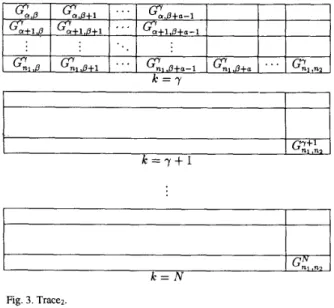
using Trace2 as follows to collect the set of segments of the module (Fig. 3):

Trace, (G:.p, free(@)) = < G&, G&+l

,...,

Ga,p+,-l, Y

Y Y Y

Ga+l,p 3 Ga+l,p+l).

.

' 1 Ga+l,p+a-I 7

where nl is the maximum row index of segments on the y-plane in the current free(@) and n2 is the maximum column index of

segments on the y-plane in the current free(@) when

a

= nl.

The processor allocation procedure is greedy, such that n l , n2 can be determined by this greedy procedure:

Step I : Let m = 1.

Step 2: Find a free segment which is minimal, G&, =

min V;ee (O)}.

Step 3: Construct the module C , = Tracez ( GL,p, fiee(O)). Step 4: Iffree(@) # 0 then m = m

+

1 goto Step 2 else stop.

k = r

I

GE .n2

I

k = N

Fig. 3. Tracez.

THEOREM 4.1. The processor allocation Procedure 4.1 is compatible with its schedule

n(l)

= ai

+

bj

+

ck, a

+

b > c,

and b = c.

PROOF.

[modulo-c]. Segments derived by gcd-partitioning must be modulo-c.

[isomorphic]. Let V I = ail

+

bjl

+

ckl and v2 = ai2

+

bj2

+

ckz be

two time-tags whose index vectors are on the same (p, q) locations about their segments G;;,~, , G&, , respectively. From the fact that every segment is a c x 1 matrix, we have v2 = a(il+ i'c)

+

bj,

+

ck2. From b = c, we have v2 - V I = ai'c

+

c(iz - j l )

+

c(k2

-

kl) = (ai'

+

j 2

-

j l

+

k2

-

kl)c. Thus, mod(y, I G ~ ; , ~ ~ I) = m ~ d ( v ~ , l G L : , ~ , I), where I = I = c.

Now we can say that every segment derived by Procedure 4.1 is isomorphic to all others.

[elementary]. Because every segment is isomorphic to all others, if two time-tags v1 and v2 are not on the same (p, q) location, then v1 # v2. We now want to prove that no two

time-tags in a module with the same (p, q) location are equal. From the module constructed by Tracez, as shown in Fig. 3 , let v = mc

+

r E G&.

Letv, = m , c + r E ~ , ' , ~ + , . t h e n v , = ( m + l ) c + r . Let v2 = mtc

+

r E G&+.-, then v 2 = ( m

+

Q

-

1)c

+

r . Let v3 = m,c

+

r E G:+,,~ then v3 = ( m

+

Q ) C

+

r. Letv, = m , c + r E ~ ~ , , ~ t h e n v , = ( m + m : a ) c + r ,

where mi> 0.

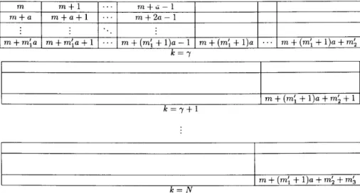
All other formulae can be derived similarly. The quotients of dividing the time-tags vl s by c with remainder r are shown in Fig. 4, from which we can see that all time-tags with the same (p, q) location are not equal, because they have different quotients. Hence every module derived by Tracez of Procedure 4.1 is elementary, Le., the processor allocation Procedure 4.1 is compatible with its schedule

0

THEOREM 4.2. The minimum number of PES required for the

n(l)

= ai

+

bj

+

ck.

schedule

n(l>

= ai

+

bj

+

ck, a

+

b > c, and b = c is

PROOF. Fig. 5 is the (k = I)-plane of a DG. The slanted lines represent a time hyperplane with the normal vector [a c elT

projected on the (k = 1)-plane. They pass through the nodes (represented by black nodes in Fig. 5) belonging to the modulo set 4(r). From left to right, we have the following observations:

there are a lines each of which passes through only one node; there are a lines each of which passes through two nodes; there are a lines each of which passes through

$

-1 nodes; there are N

-

a

(4-1)

lines each of which passes there are a lines each of which passes through

$

-1 nodes; there are a lines each of which passes through only one node. Because all the nodes on a time hyperplane are executed at the same time, they are assigned the same time-tag. These nodes with the same time-tag must be allocated to different PES. Therefore, in order to find PEmin, we need to find the hyperplane, say ~ which contains the maximum number of

nodes. We project the nodes of g i n the k-direction onto the (k = 1)-plane. These nodes should be projected onto the

(8)

690

m m + a m+m;a

IEEE TRANSACTIONS ON COMPUTERS, VOL. 44, NO. 5, MAY 1995

m + 1 . . . m + l z - l m + a + 1

. . .

m + 2 a - 1 m + m ; a + 1 ... m + ( m ; + l ) a - 1 m + ( m ; + l ) a . . . m + ( m ; + l ) a + m ; / / / //

7-

...

I m

+

(mi

+

1).

+

m;

+

mj k = N

Fig. 4. The quotients obtained by dividing the time-tags in all segments of a module by c for the case of b = c.

necessary to select N slanted lines for which the total number of black nodes passed through is maximal. From the above observations, the selection is as follows: If

4

is an

' odd number then there are

(N

-

a($ - 1)) lines each of which has

4

nodes, 2a lines each of which has

4 -

1 nodes, 2a lines each of which has

$

-

2 nodes, 2a lines each of which has

$

-

Le]

nodes. Thus the total number of nodes of %is

(N - a($ - 1))$+ 2a(

($

- 1)

+

($

-

2) + e . . +

($

-

161)

)

=

$

-

aL$][el.

Similarly, if

$

is an even number then there are (N

-

a($ -1)) lines each of which has

$

nodes, 2a lines each of which has

4

-1-nodes,

2a lines each of which has

$

-2 nodes, 2a lines each of which has

$

-

$

+1 nodes,

a lines each of which has

4

-

2

nodes. Thus the total number of nodes of His

0

THEOREM 4.3. Procedure 4.1 can always design a locally connected, space-optimal regular array f o r any SURE with

a linear schedule

n(l)

= ai

+

bj

+

ck, a

+

b > c , and b = c .

PROOF: From Procedure 4.1, we know that nodes on every plane, fkom the (k = 1)-plane to the (k = N

-

( a 4

- 1))-plane, can be allocated to

4

PES. However, nodes on the (k = N

-

a

(4

- 1)

+

l)-pIane can be allocated only to

(4

-

1) PES, because thls plane has only a($ - 1) columns of index vectors which are hee; the others have already been allocated. Similarly, the nodes on the next 2a - 1 k-planes can be allocated to

(4

- 1) PES, and then there are 2a k-planes which can be allocated to

(4

- 2) PES, and so on, until all N k-planes are allocated. If

4

is an odd number then the number of PES used is:

PEused

= (N - a($ - 1))$+2a(($ - 1)

+

($

- 2)

+...+

(4

-I$]))

Similarly, if

$

is an even number, then the number of PES

(9)

TSAY AND CHANG: DESIGN OF SPACE-OPTIMAL REGULAR ARRAYS FOR ALGORITHMS WITH LINEAR SCHEDULES

k = y + l

k = N Fig. 6 . Trace?.

B. Procedure for a = b

n(Z)

= ai

+

bj

+

ck, where a

+

b > c and a = b, a space- optimal regular array can always be obtained by partition- ing every ij-plane of the DG of the SURE into several c x 1

segments. Each module is constructed by using TraceS as follows to collect the set of segments of the module (Fig. 6):

y+u-I y+u-l y+a-1 y+u-l

G , Y ~ - '

3 G,Y:;f' 1 . . 9 GnI ,p , p + c 9 Gnl , p + 2 c 3 ' ' 3 Gn, .n2

G:l:n: 9 G;Tn":' 9 '

.

.* G&, > 3

where nl is the maximum row index of segments on the y- plane in free(@) and n2 is the maximum column index of segments on the y-plane in free(@) when

a

= nl and is

equal to

p

+

me. The processor allocation procedure is

greedy such that n l , n2 can be procedure:

Step 1: Let m = 1.

691

determined by this greedy

Step 2: Find a free segment which is minimal, G& = Step 3: Construct the module G , = Trace3 (G&, free(@)). Step 4: Iffree(@) # 0 then m = m

+

1 goto Step 2 else stop.

minCfree ( O ) ] .

THEOREM 4.4. The processor allocation Procedure 4.2 is

compatible with its schedule

n(r>

= ai

+

bj

+

ck, a

+

b > e, and a = b.

0

THEOREM 4.5: The minimum number of PES required for the PROOF: The proof is similar to that for Theorem 4.2.

schedule

n(l)=

ai

+

bj

+

ck, a

+

b > e, and a = b is PE,,, = -

[+p1.,

{+-pi

, if

+,

pi

where k { 0, , otherwise

PROOF. Fig. 7 is the (k = 1)-plane of a DG. The slanted lines represent a time hyperplane with the normal vector [a a cIT

projected onto the ( k = 1)-plane. These slanted lines pass through black nodes which belong to modulo set # r ) . As- sume that H is the time hyperplane which contains the maximum number of nodes. These nodes when projected onto the (k = 1)-plane should be on the positions of black nodes. The number of slanted lines which cover these projected nodes is

]

[:

because the time-tags' difference be- tween two adjacent slanted lines is ac and the time tags' dif- ference between two adjacent k-planes is e. However, it can be observed from Fig. 7 that the total number of slanted lines is Therefore, the total number of nodes on Hcan be calculated by selecting

[q

slanted lines for which the total number of black nodes passed through is maximal. Let

If 1 is an even number, then we have

PE,, =

$

- c

( (

2 1

+

2

+...++))

=

$-

- c[31[?1;

otherwise, we have

PE,, =

$

- C( 2(1+ 2

+...+

y)

+?)

=

q

-

c[61[+l,

U

THEOREM 4.6. Procedure 4.2 can always design a locally connected, space-optimal regular array for any SURE with a linear schedule

n(o=

ai

+

bj

+

ck, a

+

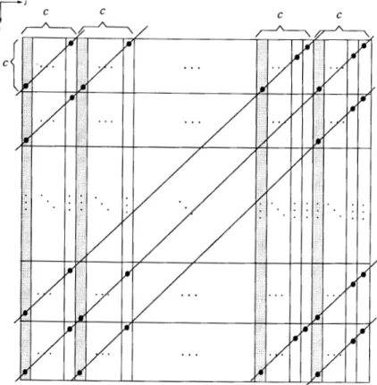
b > c and a = b.

PROOF. By Procedure 4.2, the DG of the SURE can be divided into c regions, e.g., the shaded segments in Fig. 7 and those extended in the k-direction form one of these regions. Every

(10)

692 _{IEEE TRANSACTIONS ON COMPUTERS,}_{VOL. 44,}_{NO. 5; MAY 1995}

C C C

C

Fig. 7. The ( k = 1)-plane of a DG with schedule ui

+

bj + ck, u

+

b > c, and u = b

PROOF. By Procedure 4.2, the DG of the SURE can be divided into c regions, e.g., the shaded segments in Fig. 7 and those extended in the k-direction form one of these regions. Every region is formed entirely of isomorphic segments, can be allocated independently, and will have the same number of PES. Let us consider any one region. If :is an even number, :is the number of PES for all.the nodes in the region between the ( k = 1)-plane and the (k = a)-plane, 2($-1) is the number of PES for all the nodes in the region between the ( k = a

+

1)-plane to those of the (k = 3a)-plane, and so on. Thus the number of PES used by each region is

where

On the other hand, if

I

5 I

is an odd number, then the number of PES used by each region is

Because there are c regions in the DG, the number of PES 0

used by Trace3 is PEused =

$

-

c[41[?1.

EXAMPLE 4.1. [matrix multiplication] The dependence ma- trix D for matrix multiplication [21] can be written as

.-E

;

8].

and its DG is shown in Fig. 8(a) ( N = 6). Its corresponding optimal linear schedule is

n(r)

= i

+

j

+

k. Thus by applying Procedure 4.1 (or Procedure 4.2), the time-tags of all index vectors on every ij-plane can be gcd-partitioned into several 1 x 1 segments. The module is then constructed by Trace2 of Procedure 4.1 (or Trace3 of Procedure 4.2), as shown in Fig. 8(b). By mapping each module onto one PE, a space- optimal regular array can be constructed, as shown in Fig. 8(c). If we adopt the linear space mapping, then N = 36

PES is necessary. But Procedure 4.1 (or Procedure 4.2) can reduce the PEused to

(11)

TSAY AND CHANG: DESIGN OF SPACE-OPTIMAL REGULAR ARRAYS FOR ALGORITHMS WITH LINEAR SCHEDULES 693

k = l

Fig. 8(a). The DG for matrix multiplic

k = 2

k = 6 :ation (N = 6).

k = 5

k = 6

Fig. 8(b). The processor allocation for matrix multiplication by Procedure 4.1 (or Procedure 4.2).

advance a maximum concurrent set for a given linear schedule in order to design space-optimal regular mays. The proposed processor allocation procedures ensure that no two nodes scheduled at the same time are mapped onto the same PE (Theorem 3.1) and that all PES are active simultaneously at some one time instance (Theorem 3.2). Second, for a given linear schedule

n(I)

= ai

+

bj

+

ck, 1 I a I b I c, for an SURE, two cases were studied: a

+

b I c and a

+

b > c. In the former case, a space-optimal design can always be obtained by Procedure 3.1; the number of PES used is

$.

The resulting array has the advantages of local connection, load balance,

v

Fig. 8(c). The space-optimd regular array for matrix multiplication.

simple control, and space optimality. For the latter case, $becomes the upper bound of PEmin. We also discussed two special cases of a

+

b

>

c, a = b and b = c. By Procedures 4.1 ( b = c ) and 4.2 (a = b), space-optimal regular arrays can also be obtained for these cases. The closed form expressions for PEmin are also given for the cases of b = c and

a

= b in Theo-

rems 4.2 and 4.5, respectively. Although only three dimensional algorithms with linear schedules are discussed here, the method proposed in this paper can easily be extended to higher dimensional algorithms. More research on the topic of space- optimal design should be pursued; one important project would be to solve the problem of space-optimality for linear schedule

n(Z)

= ai

+

bj

+

ck with a

+

b > c and its closed form expressions for PE,in.

ACKNOWLEDGMENTS

We would like to thank the referees for their constructive and helpful comments. This research was supported by the National Science Council of the Republic of China under con- tract NSC-83-0408-E-009-044.

REFERENCES [ l ]

[2] [3]

H.T. Kung and C.E. Leisenon, “Systolic arrays for VLSI,” Proc. 1978

Soc. for Industrial and Applied Math., pp. 256-282, 1979.

J.A.B. Fortes and B.W. Wah, “Systolic mays1From concept to im- plementation,” Computer, pp. 12-17, July 1987.

J.C. Tsay and P.Y. Chang, “Some new designs of 2D array for matrix multiplication and transitive closure,” IEEE Trans. Parallel and Dis-

(12)

694 IEEE TRANSACTIONS ON COMPUTERS, VOL. 44, NO. 5. MAY 1995

ACKNOWLEDGMENTS [23] A. Benaini and Y. Robert, “Spacetime-minimal systolic arrays for

gaussian elimination and the algebraic path problem,’’ Parallel Com-

puting, vol. 15, pp. 21 1-225, 1990.

P. Clauss, c . Mongenet, and G.R. Pemn, “Synthesis of size-optimal toroidal arrays for the algebraic path problem: A new contribution,”

Parallel Computing, vol. 18, pp. 185-194, 1992.

P. Clauss, C. Mongenet, and G. Pemn, “Calculus of space-optimal

We would like to thank the referees for their constructive and helpful comments. This research was supported by the National Science Council of the Republic of China under con-

[24]

[25] : NSC-83-0408-E-009-044.

REFERENCES

H.T. Kung and C.E. Leiserson, “Systolic arrays for VLSI,” Proc. I978

Soc. f o r Industrial and Applied Math., pp. 256-282, 1979.

J.A.B. Fortes and B.W. Wah, “Systolic arrays)From concept to im- plementation,” Computer, pp. 12-17, July 1987.

J.C. Tsay and P.Y. Chang, “Some new designs of 2D array for matrix multiplication and transitive closure,” IEEE Trans. Parallel and Dis-

tributed Systems. Submitted for publication.

P.Y. Chang and J.C. Tsay, “A family of efficient regular arrays for algebraic path problem,” IEEE Trans. Computers, vol. 43, no. 7, pp. 169-777, July 1994.

J.C. Tsay and P.Y. Chang, “Design of efficient regular arrays for ma- trix multiplication by two step regularization,” IEEE Trans. Parallel

and Distributed Systems, vol. 6, no. 2, pp. 215-222, Feb. 1995.

V. Van Dongen and P. Quinton, “Uniformization of linear recurrence equations: A step towards the automatic synthesis of systolic arrays,”

Proc. Int’l Cor$ Systolic Arrays, pp. 473-482, 1988.

S.Y. Kung, VLSI Array Processor, Prentice Hall, Englewood Cliffs, N.J., 1988.

Y.W. Wong and J.M. Delosme, “Broadcast removal in systolic algo- rithms,” Proc. Int’l Con$ Systolic Arrays, pp. 4 0 3 4 1 2 , 1988.

S.Y. Kung, S.C. Lo, and P.S. Lewis, “Optimal systolic design for the transitive closure and the shortest path problems,” IEEE Trans. Com-

puters‘vol. 36, pp. 6 0 3 4 1 4 , May 1987.

C. Choffrut and K. Culik II, “Folding of the plane and the design of sys- tolic arrays,” Irzfomtion Processing Leners, vol. 17, pp. 149-153, 1983. J.M. Delosme and I.C.F. Ipsen, “Efficient systolic arrays for the solu- tion of toeplitz systems: An illustration of a methodology for the con- struction of systolic architectures in VLSI,” Proc. Int’l Workshop on

Systolic Arrays, pp. 3 7 4 5 , 1986.

J.H. Moreno and T. Lang, “Graph-based partitioning of matrix algo- rithms for systolic arrays: application to transitive closure,” Pruc. Int’l

Conf. Parallel Processing, pp. 28-31, 1988.

P. Quinton, “Automatic synthesis of systolic arrays from uniform recurrent equations,” Proc. Int’l Symp. Computer Architecture, pp.

S.K. Rao, “Regular iterative algorithms and their implementations on processor arrays,” PhD thesis, Stanford Univ., 1985.

D.I. Moldovan and J.A.B. Fortes, “Partitioning and mapping algo- rithms into fixed size systolic arrays,” IEEE Trans. Computers, vol.

35, pp. 1-12, Jan. 1986.

W.L. Miranker and A. Winkler, “Spacetime representations of compu- tational structures,” Computing, vol. 32, pp. 92-1 14, 1984. P.Z. Lee and Z.M. Kedem, “Synthesizing linear array algorithms from nested for loop algorithms,” IEEE Trans. Computers, vol. 37, pp, 1,578-1,598, Dec. 1988.

V.P. Roychowdhury and T. Kailath, “Subspace scheduling and parallel implementation of non-systolic regular iterative algorithms,” J . of

VLSISignal Processing, vol. I , pp. 127-142, 1989.

V. Van Dongen, “Quasi-regular arrays: Definition and design method- ology,” Proc. Int’l Cor$ on Systolic Arrays, pp. 126-135, 1989.

W. Shang and J.A.B. Fortes, “Time optimal linear schedules for algorithms with uniform dependencies,” IEEE Trans. Computers, vol. 40,

pp. 723-742, June 1991.

P. Cappello, “A processor-time-minimal systolic array for cubical mesh algorithms,” IEEE Trans. Parallel and Distributed Systems, vol. 3 , pp. 4-13, Jan. 1992.

C.J. Scheiman and R.P. Cappello, “A processor-time-minimal systolic array for transitive closure,” IEEE Trans. Parallel and Distributed Svstems. vol. 3. DO. 257-269. Mav 1992.

208-214, 1984.

mappings of systolic algorithms on processor arrays,” J. VLSI Signal

Processing, vol. 4, pp. 27-36, 1992.

J. Bu and E.F. Deprettere, “Processor clustering for the design of optimal fixed-size systolic arrays,” Proc. Int’l Con$ on Application Spe-

cific Arruy Processors, pp. 4 0 2 4 1 3 , Sept. 1991.

[26]

[27] A Date, T Risset, and Y Robert, “Synthesizing systolic arrays some recent developments,” Proc Int’l Conf on Application Specific Array Processors, pp 372-386, Sept 1991

Y. Wong and J M Delosme, “Space-optimal linear processor alloca- hon for systolic arrays synthesis,” Proc Sixth Int’l Parallel Processing

Symp , pp 275-282, Mar 1992

Y C Hou and J.C Tsay, “Equivalent transformations on systolic design represented by generating functions,” J Information Science and Eng , vol 5, pp 229-250, 1989

S K Rao and T Kailath, “Regular iterahve algonthms and their im- plementation on processor arrays,’’ Proc IEEE, vol 76, pp 259-269, Mar 1988

P Y Chang and J C Tsay, “Timespace mapping for regular arrays,”

Parallel Algorithms and Applicationr Submitted for publication

E M Reingold, J Nieverglt, and N Deo, Comb~natorial Algorithms Theory and Practice, Prentice Hall, Englewood Cliffs, N J , 1977 P S. Lewis and S Y Kung, “An optimal systolic array for the algebraic path problem,” IEEE Trans Computerr, vol 40, pp l W 1 0 5 , Jan 1991 1281 [29] [30] [31] [32] [33]

Jong-Chuang Tsay received the MS and PhD degrees in computer science from the National Chiao-Tung University in the Republic of China in 1968 and 1975, respectively He has been on the faculty of the Department of Computer Engineenng at the National Chiao-Tung University since 1968 and is currently a professor in the Department of Computer Science and Information Engineenng His research interests include systolic arrays, parallel computation, and computer-aided typesetting.

Pen-Yang Chang received the MS degree in computer science from the National Chiao-Tung Uni- versity in the Republic of China in 1986 He has been an assistant researcher in the Telecommunca- hon Laboratones of the Ministry of Communication in the R 0 C since 1987 and is a PhD candidate at the Institute of Computer Science and Information Engineenng at the National Chiao-Tung University His research interests include systolic arrays and multimedia information systems