Bayesian Classification for Data From the
Same Unknown Class
Hung-Ju Huang and Chun-Nan Hsu, Member, IEEE
Abstract—In this paper, we address the problem of how to
clas-sify a set of query vectors that belong to the same unknown class. Sets of data known to be sampled from the same class are naturally available in many application domains, such as speaker recogni-tion. We refer to these sets as homologous sets. We show how to take advantage of homologous sets in classification to obtain im-proved accuracy over classifying each query vector individually. Our method, called homologous naive Bayes (HNB), is based on the naive Bayes classifier, a simple algorithm shown to be effec-tive in many application domains. HNB uses a modified classifi-cation procedure that classifies multiple instances as a single unit. Compared with a voting method and several other variants of naive Bayes classification, HNB significantly outperforms these methods in a variety of test data sets, even when the number of query vec-tors in the homologous sets is small. We also report a successful application of HNB to speaker recognition. Experimental results show that HNB can achieve classification accuracy comparable to the Gaussian mixture model (GMM), the most widely used speaker recognition approach, while using less time for both training and classification.
Index Terms—Classification, machine learning, naive Bayes
classifier, speaker recognition.
I. INTRODUCTION
T
HE PROBLEM of classification is actively researched in pattern recognition and machine learning. Research on classification centers on developing classification systems that correctly recognize unknown patterns. In classical pattern recognition [1], the input to a classifier is a single query vector and the output is a class label for that query vector. However, suppose we know that a set of query vectors belong to the same class. For example, a botany student discovers a plant she has never seen before. In order to identify the plant’s species, she collects several leaves to provide input to a classifier. Obvi-ously, the output class labels for these leaves should all be the same. We refer to a set of query vectors sampled from the same class as a homologous set. Such samples are readily available in many other applications, such as speaker recognition [2]. The combined information from multiple query vectors in aManuscript received March 14, 2001; revised August 2, 2001, October 9, 2001, and November 6, 2001. This work was supported in part by the National Science Council of Taiwan, R.O.C., under Grant NSC 89-2213-E-001-031. The speech data set was courtesy of the Speech Processing Laboratory, Department of Communication Engineering, National Chiao-Tung University, Hsinchu, Taiwan, R.O.C. This paper was recommended by Associate Editor D. Cook.
H.-J. Huang is with the Department of Computer and Information Science, National Chiao-Tung University, Hsinchu 300, Taiwan, R.O.C.
C.-N. Hsu is with the Institute of Information Science, Academia Sinica, Nankang 115, Taipei City, Taiwan, R.O.C. (e-mail: [email protected]; http://chunnan.iis.sinica.edu.tw).
Publisher Item Identifier S 1083-4419(02)00696-9.
homologous set might be used to aid the classification process. However, standard classification algorithms are not designed to take advantage of this knowledge.
Due to the robust performance and simple implementation, the naive Bayes classifier has become a popular classification tool in recent years. Many applications prefer the naive Bayes classifier because of its simplicity. In spite of its simplicity, the naive Bayes classifier achieves comparable performance with popular classifiers such as C4.5 [3],and constantly outperforms competing algorithms, on average, in experiments reported in the literature [4]. Remarkably, in KDD-CUP-97, two of the top three contestants are based on the naive Bayes classifier [5]. Also, Domingos and Pazzani [6] reported an experiment that compared the naive Bayes classifier with several classical learning algorithms on a large ensemble of data sets. Their results also show that the naive Bayes classifier is a good classification tool.
Previous work has focused on improving the accuracy of naive Bayesian classifiers with a single query vector. No past study has been devoted to the problem of classifying homologous sets with the naive Bayes classifiers. In this paper, we present a method called homologous naive Bayes (HNB), which allows for the efficient classification of homologous sets by the naive Bayes classifier. We empirically compared this method with voting and several other extensions of the naive Bayes classifier, which we will describe later. Experimental results show that HNB outperforms all other methods. Further analysis shows that, to improve the classification accuracy, the other extension methods require large homologous sets, while HNB can significantly improve the result accuracy even when there is only one pair of query vectors in each homologous set. Our application of the HNB method to speaker recognition proved to be successful. In this type of application, we usu-ally have prior information that large sets of query vectors come from the same unknown speaker.
The remainder of this paper is organized as follows: Section II reviews the naive Bayes classifier. Section III presents several approaches to classifying homologous sets. Section IV empiri-cally compares the performance of the different methods. Sec-tion V reports an applicaSec-tion of HNB to speaker recogniSec-tion. Finally, Section VI contains the summary of conclusions.
II. NAIVEBAYESCLASSIFIERS
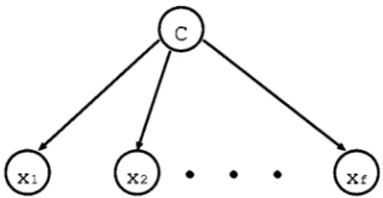
The naive Bayes classifier is based on the simplifying as-sumption that the feature values are conditionally independent given the class label [7]. Fig. 1 gives a graphical depiction. A naive Bayes classifier classifies a query vector of predictive 1083–4419/02$17.00 © 2002 IEEE
Fig. 1. Naive Bayes classifier, where the predictive features (x ; x ; . . . ; x ) are conditionally independent given the class attribute (c).
features by selecting class that maximizes the posterior prob-ability
(1)
where is a predictive feature (variable) in and is the class-conditional density of given class . Let denote the vector whose elements are the parameters of the density of . In a Bayesian learning framework, we assume that can be learned from a training data set. This estimation is at the heart of training in the naive Bayes classifier.
The naive Bayes classifier can handle discrete variables and continuous variables when assuming that their priors are Dirichelet distribution and normal distribution, respectively [8]. In the following section, we describe the learning procedures of a naive Bayes classifier with different types of variables.
A. Naive Bayes Classifier With Discrete Variables
Suppose is a discrete variable with possible values. In principle, the class label of the data vector dictates the prob-ability of the value of . Thus, the appropriate probprob-ability distri-bution function is a multinomial distridistri-bution and its parameters are a set of probabilities , such that for each
pos-sible value , and . Now, let
, a Dirichlet distribution [9] with parame-ters as the prior for . Given a training data set, we
can update using its expected value
(2) where is the number of the training examples belonging to
class , is the number of class examples whose ,
and . Since a Dirichlet distribution is conjugate to multinomial sampling, after the training, the posterior distri-bution of is still a Dirichlet, but with the updated parameters being for all . This property allows us to incrementally train the naive Bayes classifier.
In practice, we usually choose the Jaynes prior [10]
for all and have . However, when
the training data set is too small, this often yields
and impedes the classification. To avoid this problem, another popular choice is for all . This is known as smoothing or Laplace’s estimate [11].
B. Naive Bayes Classifier With Continuous Variables
If is a continuous variable, a conventional approach is to
assume that , where is the
probability distribution function of a normal distribution. In this case, training involves learning the parameters and from the training data [8]. This approach has been shown to be less effective than discretization when is not normal, and dis-cretization is often used. Generally, disdis-cretization involves par-titioning the domain of into intervals as a pre-processing step. Then we can treat as a discrete variable with possible values and conduct the training and classification as described in Section II-A.
More precisely, let be the th discretized interval. Training and classifying in the naive Bayes classifier with discretization
is to use as an estimate of in (1) for each
continuous variable. This is equivalent to assuming that after discretization, the class-conditional density of has a Dirichlet prior. This assumption is called Dirichlet discretization
assump-tion. This assumption holds for all well-known discretization
methods, including ten-bin, entropy-based [12], among others. (see [13] for a comprehensive survey).
Since it has been shown to be less effective than discretization when the distribution of a continuous variable is not normal, we must select a discretization method for our experiments. In our previous work [14], we explained why well-known discretiza-tion methods, such as entropy-based, bin- and ten-bin, work well for naive Bayes classifiers with continuous variables, re-gardless of their complexities. In this paper, we used the simple method “ten-bin” for partitioning continuous variables in all of our experiments. This method merely divides the range of ob-served values for a variable into ten equal-size bins. However, other discretization methods can also be used.
III. CLASSIFYING AHOMOLOGOUSSET
We start by showing that a classifier must deliberately take ad-vantage of the knowledge that all data have the same unknown class label; otherwise, the knowledge will not improve the ex-pected accuracy, and this is generally the case regardless of the number of query vectors in the homologous set and the number of classes that we want for classifying the data. Consider a clas-sifier which classifies one query vector into one of the classes, with accuracy . Suppose this classifier classifies query vec-tors individually. The expected value of the accuracy can be de-rived from the following:
(3)
(4)
(5)
(7)
(8)
(9) (10) (11) where denotes the event that there are query vectors which are classified incorrectly, and the expected value is the weighted average of the probabilities of . “ ” is replaced by from (8) and (9) and the binomial theorem [15] is used to derive (10) from (9).
On the other hand, suppose we know that the vectors ac-tually belong to the same class and take them as one object. We therefore classify this object using the same classifier. The ex-pected value of the accuracy is
(12)
(13) (14) The expected values of the above two cases are the same. This implies that the prior information, indicating that query vectors come from the same class, does not automatically improve the accuracy.
A. Voting, Averaging, Maximum, and Their Variations
There are several intuitive extensions for the naive Bayes clas-sifier to classify homologous sets. One method is voting, which uses the naive Bayes classifier to classify each member in the homologous set and selects the class label predicted most often.
Let be a homologous set of query vectors
with the same unknown class label and each query vector
in has features . We assume that
are drawn independently,1 and the symbol denotes the prior information that all members in the homologous set have the same unknown class label. According to the Bayesian decision theory, we should classify this homologous set by selecting the
class that maximizes , the probability of given
and . We can derive four “extension” methods to estimate for classifying the query vectors in a homologous set.
1) Avg
The “Avg” method estimates for each
and averages the results to obtain as follows:
(15) 1A feature vector may depend on other feature vectors in real situations if they come from the same class.
2) Local Avg (LAvg)
In this method, for each feature , we compute the av-erage of the class-conditional probability of all members and use the result as the class-condi-tional probability of the feature . Then we can
obtain as follows:
(16)
3) Max
The “Max” method estimates for each
and selects the maximum probability as as
follows:
(17)
4) Local Max (LMax)
In this method, the class-conditional probability for each feature is estimated by selecting the
maximum among all members . Then
we can obtain as follows:
(18)
The classification rule of the above methods is to pick the class
that maximizes .
B. Homologous Naive Bayes (HNB)
The above four methods are based on the idea that we can
combine the estimation of to obtain , by
av-eraging or by selecting the maximum values. In fact, we can derive a method purely from the Bayes rule and independence assumptions as follows: (19) (20) (21) (22) (23) (24) (25) We can simplify (22) and (23) because of the assumption that all members in are drawn independently. Since is
TABLE I TESTDATASETS
logically implied by the event that are of class , and we can reduce (23) and (24). For the sake of being concise, we rewrite (24) as (25). Finally, since the naive Bayes classifier assumes that all features are independent given class , (25) can be decomposed by the following equations:
(25)
(26)
(27) (28)
Therefore, the classification rule is to pick class that max-imizes (28). We call this method homologous naive Bayes
(HNB). Note that the training procedure of the above methods
remains unchanged as the standard naive Bayes classifier described in Section II.
IV. EMPIRICALRESULTS
To evaluate the methods described in Section III, we selected several data sets from UCI ML repository [16] for our experi-ments. Results obtained with these data sets are widely reported in the machine learning literature. Table I lists information about each set.
A. Classifying Small Homologous Sets
In the first experiment, we investigated the performance of the methods when there are two or three elements in a
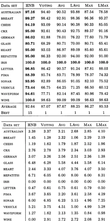
homolo-TABLE II
AVERAGEACCURACIES(TOP)ANDSTANDARDDEVIATIONS(BOTTOM) USINGDIFFERENTNAIVEBAYESCLASSIFICATIONMETHODSWHEN
THESIZE OF AHOMOLOGOUSSET ISTWO
gous set. We first partitioned the data by class. Then, each class group was divided into five parts for running fivefold cross vali-dation [17]. In each test set, we randomly drew two or three test examples to form a homologous set in our test data. Then, we trained the naive Bayes classifier with the training sets and used the six different methods to classify the test data for each data set.
We report the average and standard deviations of the accu-racies after running fivefold cross validation on each data set. Table II gives the results of classifying homologous sets with two query vectors and Table III gives the results of classifying homologous sets with three query vectors. Located at the top of these two tables are the accuracies achieved by different methods, whereas at the bottom are the standard deviations of the accuracies. The results in Table II reveal that HNB outperforms the other methods in all data sets except one
TABLE III
AVERAGEACCURACIES(TOP)ANDSTANDARDDEVIATIONS(BOTTOM) USINGDIFFERENTNAIVEBAYESCLASSIFICATIONMETHODSWHEN
THESIZE OF AHOMOLOGOUSSET ISTHREE
(Wine, “LAvg”). In this table, we also list the accuracies of the standard naive Bayes classifier (SNB), which classifies one query vector at a time. When comparing the effectiveness of the standard naive Bayes classifier with others, we see that HNB achieves remarkable improvement. In contrast, the improvement by other methods is not only minor, but in some cases, the performance is worse than the SNB.
Let the accuracy of a classifier given a query vector be . Suppose there are two query vectors with the same unknown class label and the voting method is applied to classify them. In our implementation of voting, if the two results disagree, we randomly pick one as the final result. In this case, the expected
Fig. 2. Accuracies in classifying homologous sets using different sizes in the data set “Chess.”
accuracy is 0.5 when one of the results is correct. Therefore, the expected accuracy of the classifier when using voting is
This shows that when we only know of two query vectors having the same unknown class label (i.e., the size of a homol-ogous set is two), the expected accuracy will not be improved by voting. The experimental results given in Table II match our analysis. The accuracies of the two methods (SNB and voting) in most data sets are close.
In Table III, we grouped three query vectors in a homologous set. The results show that though the performance of voting is improved, the performance of HNB is improved even more and becomes the best of all methods for all data sets. In the next subsection, we discuss how the performance of HNB scales to increasing sizes of homologous sets.
B. Classifying Large Homologous Sets
A large homologous set increases the chances that a naive Bayes classifier correctly classifies a majority of the query vectors, thus ameliorating the performance of voting. In order to compare the performance of HNB and voting with different sizes of homologous sets, we selected three large data sets (“Chess,” “Letter,” and “Waveform,” see Table I for their information) and repeated the same procedure as in the first experiment for different sizes of homologous sets (from 1 to 50 or 100). Note that when the size of a homologous set is 1, both HNB and voting are reduced to an SNB. This case serves as the baseline for performance evaluation.
Figs. 2–4 plot the resulting curves, which show that the per-formance of voting improves as the size of homologous sets in-creases, but the curves of HNB grow faster. HNB reaches per-fect accuracy with less than 20 query vectors in the homologous sets. In contrast, voting requires many more vectors in order to reach the same performance.
Fig. 3. Accuracies in classifying homologous sets using different sizes in the data set “Letter.”
Fig. 4. Accuracies in classifying homologous sets using different sizes in the data set “Waveform.”
V. APPLICATION INSPEAKERRECOGNITION
Speaker recognition [15] is the process of automatically recognizing who is speaking on the basis of information obtained from speech waves. HNB is ideal for this task because we are easily able to sample a set of query vectors from the same unknown speaker. Since a large number of query vectors can be extracted from a short sentence, and obviously those vectors come from the same speaker, a speaker recognition system should take advantage of this information. Speaker recognition can be divided into two categories: “open-set” and “close-set.” In “open-set” situations, the test speaker may not be registered and the system must identify that speaker as “unknown,” while in “close-set” situations, the test speaker must be in the set of registered speakers. Speaker recognition can also be categorized according to its text dependency [18]. In text-dependent cases, speakers provide utterances of the same text for both training and testing. On the other hand, text-independent can use same or different text for training and testing. In this paper, we applied our work to a close-set, text-independent speaker recognition task.
A. Experiments
In this section, we compared HNB with voting in a speaker recognition task. The database used for the experiments
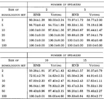
TABLE IV
ACCURACIES OF THEAPPLICATION TOSPEAKERRECOGNITION
reported in this paper is a subset of the TCC-300, a speech database in Mandarin Chinese maintained by many research institutes in Taiwan. We used the speech data recorded at the National Chiao-Tung University. All speech signals were digitally recorded in a laboratory using a personal computer with a 16-bit sound blaster card and a headset microphone. The sampling rate was 16 kHz. A 30-ms Hamming window was applied to the speech every 10 ms, allowing us to obtain 100 feature vectors from 1-s speech data. For each speech frame, both a twelfth-order linear predictive analysis and a log energy analysis were performed. We filtered the feature vectors whose log energy values were lower than 30. This can be viewed as a silence-removing process. A feature vector for training or testing contained the 12 linear predictive parameters. More than ten sentences were recorded from each subject speaker, and from each sentence, more than 4000 feature vectors were extracted.
The experimental procedure was conducted as follows. We randomly selected five sentences for each speaker, one for testing and the others for training. Then, we randomly selected 1000 feature vectors from each sentence. Hence, for each speaker there were 4000 feature vectors for training and 1000 feature vectors for testing. We ran fivefold cross validation on different numbers of speakers and different sizes of homolo-gous sets. We report the average and standard deviations of the accuracies in Table IV. The accuracies for both methods (HNB and voting) improve significantly in all cases when the sizes of homologous sets increase. However, HNB reaches high accuracy faster than voting. This is consistent with the results in Figs. 2–4.
B. Gaussian Mixture Model (GMM)
The most common and successful approaches to close-set, text-independent speaker recognition include the Gaussian mixture model approach (GMM) [19] and the hidden Markov
model approach (HMM) [20]. In recent speaker recognition evaluations carried out by the National Institute of Standards and Technology (NIST), the best GMM-based systems have outperformed the HMM-based systems [21]. In this section, we will briefly review the GMM approach to speaker recog-nition. Then, we will empirically compare HNB and GMM in Section V-C.
A Gaussian mixture density is a weighted sum of compo-nent densities and is given by the form [19]
where is a -dimensional random vector, ,
is the component density and ,
is the mixture weight. Each component density is a -variate Gaussian function of the form
with mean vector and covariance matrix . The mixture weights must satisfy the constraint that
The complete Gaussian mixture density is parameterized by the mean vectors, covariance matrices, and mixture weights from all component densities. These parameters are collectively rep-resented by the notation
Then, each speaker is represented by a GMM and is referred to by his/her model parameter set . A GMM parameter set for a speaker is estimated using the standard expectation maxi-mization (EM) algorithm [22]. For a sequence of query
vec-tors , the GMM log-likelihood can be
written as
In the standard identification approach, the test speaker is recognized from a set of speakers by
Several system parameters must be tuned for training a Gaussian mixture speaker model, but a good theoretical guide for setting the initial values of those parameters has not been found. The most critical parameter is the order of the mixture. Choosing too few mixture components can produce a speaker model that cannot accurately model the distinguishing characteristics of a speaker’s distribution. Choosing too many components reduces performance when there are a large number of model parameters relative to the available training data [19].
TABLE V
ACCURACIES OFHNBANDGMMFORRECOGNIZING16 (TOP)AND
30 (BOTTOM) SPEAKERS
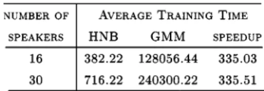
TABLE VI
AVERAGETRAININGTIME OFHNBANDGMMFORDIFFERENT
NUMBER OFSPEAKERS
C. Comparisons Between HNB and GMM
In this section, HNB is empirically compared with the most successful statistical model (GMM) for speaker recognition. The experimental procedure is the same as in Section V-A and the same data set is used. for GMM is used in our experiments. This setting is suggested in [19] and works well in our data sets. We also ran fivefold cross validation on two different numbers of speakers and different sizes of homologous sets. One hundred test data represents 1 s of speech data. We reported the average accuracies and their standard deviation. We also reported the average CPU time ticks taken for training and classification. Table V shows the results of recognition accuracies for 16 and 30 speakers. Tables VI and VII show the average training and classification time (the size of homologous is from 1 to 600). The experiments were run on Pentium III 800 MHz PCs with 256M DRAM.
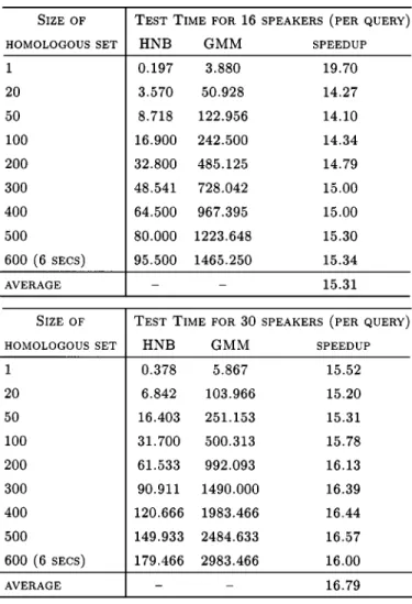
TABLE VII
TESTINGTIME OFHNBANDGMMFOR THETEST ON16 (TOP)AND
30 (BOTTOM) SPEAKERS
The results show that GMM requires smaller numbers of test vectors than HNB to reach a high accuracy. However, given more feature vectors in the homologous sets, HNB quickly catches up and reaches comparable accuracy to GMM. This is not surprising because the GMM is capable of modeling the correlations between the variables in a feature vector, but the correlations are disregarded in the naive Bayes classifier due to its independent assumption. As a result, when the size of a homologous set is 1, the accuracies of HNB will be much lower than GMM. However, HNB gains several advantages from the independent assumption. One is that the implemen-tation of HNB is much simpler than the GMM algorithm. Other advantages of HNB include the faster training and classification speeds. In our experiment, the average training speed of HNB surpasses GMM by about 355 times, and the average classification speed by about 15 (see Tables VI and VII for training time and classification time, respectively). In addition, HNB reaches high accuracies ( 99%) by using about 1 s of speech data. This shows that it is not necessary to use a very large number of query vectors in order to boost HNB’s accuracies. An interesting phenomenon here is that, though more query vectors are required in order for HNB to reach perfect accuracy, HNB’s classification speed is still faster than GMM’s speed, as shown in Table VIII.
TABLE VIII
SIZE OF AHOMOLOGOUSSET ANDCLASSIFICATIONTIME FORREACHING THEPERFECTACCURACY
Based on the discussion above, we draw the following conclu-sions on applying HNB in speaker recognition task. Since one additional second of speech is a low cost to the speakers, it is a tolerable or even favorable tradeoff in favor of HNB. Hence, if it is not too difficult to obtain speech data from the same speaker for classification, or if low-cost implementation is required, the HNB can be a useful approach.
VI. CONCLUSIONS
The naive Bayes classifier is widely used in many clas-sification tasks because its performance is competitive with state-of-the-art classifiers, it is simple to implement, and it possesses fast execution speed. In this paper, we discussed the problem of how to classify a set of query vectors from the same unknown class with the naive Bayes classifier. We showed that a classifier must deliberately take advantage of the knowledge that all data have the same unknown class label; otherwise the knowledge will not improve the expected accuracy. Then, we proposed the method HNB and compared it with several simple methods (Avg, LAvg, Max, LMax, and Voting). The experimental results show that HNB can take advantage of the prior information that all members in a homologous set have the same class label, improve accuracy, and outperform the other methods when the naive Bayes model is used.
We also compared HNB and voting for the application of speaker recognition. Experimental results show that HNB can work well on this task and is more suitable than voting. Fi-nally, HNB was compared with the GMM approach in speaker recognition. Experimental results reveal that, although HNB can reach the same level of accuracies as GMM by using about 1 s more of test speech data, HNB’s execution speed is much faster than GMM, and HNB has low implementation cost. Hence, we suggest that HNB is useful in the domain of speaker recognition and may be applied to other applications, if homologous sets are available in that problem domain.
ACKNOWLEDGMENT
The authors wish to thank anonymous reviewers for their valuable comments.
REFERENCES
[1] K. Fukunaga, Introduction to Statistical Pattern Recognition, New York: Academic, 1990.
[2] C.-H. Lee, F. K. Soong, and K. K. Paliwal, Automatic Speech and
Speaker Recognition. Norwell, MA: Kluwer, 1996.
[3] J. R. Quinlan, C4.5: Programs for Machine Learning. San Mateo, CA: Morgan Kaufmann, 1993.
[4] N. Friedman, D. Geiger, and M. Goldszmidt, “Bayesian network classi-fiers,” Mach. Learn., vol. 29, pp. 131–163, 1997.
[5] I. Parsa. (1997) KDD-CUP 1997 presentation. [Online]. Available: http://www.ncst.ernet.in/kbcs/vivek/issues/10.4/kdd/kdd.html. [6] P. Domingos and M. Pazzani, “On the optimality of the simple Bayesian
classifier under zero-one loss,” Mach. Learn., vol. 29, pp. 103–130, 1997.
[7] T. M. Mitchell, Machine Learning, New York: McGraw-Hill, 1997. [8] G. John and P. Langley, “Estimating continuous distributions in
Bayesian classifiers,” in Proc. 11th Annu. Conf. UAI, 1995, pp. 338–345.
[9] S. S. Wilks, Mathematical Statistics, New York: Wiley, 1962. [10] R. Almond, Graphical Belief Modeling. London, U.K.: Chapman &
Hall, 1995.
[11] B. Cestnik and I. Bratko, “On estimating probabilities in tree pruning,” in Machine Learning—EWSL-91, European Working Session on
Learning. Berlin: Springer-Verlag, 1991, pp. 138–150.
[12] U. M. Fayyad and K. B. Irani, “Multi-interval discretization of contin-uous valued attributes for classification learning,” in Proc. 13th IJCAI, 1993, pp. 1022–1027.
[13] J. Dougherty, R. Kohavi, and M. Sahami, “Supervised and unsupervised discretization of continuous features,” in Machine Learning:
Proceed-ings of the 12th International Conference (ML ’95). San Mateo, CA: Morgan Kaufmann, 1995.
[14] C.-N. Hsu, H.-J. Huang, and T.-T. Wong, “Why discretization works for naive Bayesian classifiers,” in Machine Learning: Proceedings of the
17th International Conference (ML 2000). San Mateo, CA: Morgan Kaufmann, 2000.
[15] S. Ross, A First Course in Probability. Englewood Cliffs, NJ: Prentice-Hall, 1998.
[16] C. Blake and C. Merz. (1998) UCI repository of machine learning databases. [Online]. Available: http://www.ics.uci.edu/~mlearn/ML-Repository.html.
[17] M. Stone, “Cross-validatory choice and assessment of statistical predi-tions,” J. R. Stat. Soc., vol. 36, pp. 111–147, 1974.
[18] H. Gish and M. Schmidt, “Text-independent speaker identification,”
IEEE Signal Processing Mag., vol. 11, pp. 18–32, 1996.
[19] D. A. Reynolds and R. C. Rose, “Robust text-independent speaker iden-tification using Gaussian mixture speaker models,” IEEE Trans. Speech
Audio Processing, vol. 3, pp. 72–83, Jan. 1995.
[20] J. de Veth and H. Bourlard, “Comparision of hidden Markov model techniques for automatic speaker verification in real-world conditions,”
Speech Commun., vol. 17, pp. 81–90, 1995.
[21] M. A. Przybocki and A. F. Martin, “NIST speaker recognition eval-uation,” in Workshop Speaker Recognition and Its Commercial and
Forensic Applications (RLA2C), Avignon, France, 1998.
[22] A. P. Dempster, N. M. Laird, and D. B. Rubin, “Maximum likelihood from incomplete data via the em algorithm,” J. R. Stat. Soc., vol. Series B, no. 39, pp. 1–38, 1977.
Hung-Ju Huang was born on August 1, 1974, in Taipei, Taiwan, R.O.C. He
received the B.S. degree in computer science and information engineering from Ta-Tung Institute of Technology, Taipei, Taiwan, in 1996. Currently, he is pur-suing the Ph.D. degree in the Department of Computer and Information Science, National Chiao-Tung University, Hsinchu, Taiwan. His main research interests include maching learning, artificial intelligence, and VLSI CAD.
Chun-Nan Hsu (M’01) received the B.S. degree in computer engineering from
National Chiao-Tung University (NCTU), Hsinchu, Taiwan, R.O.C., in 1988, and the M.S. and Ph.D. degrees in computer science from the University of Southern California, Los Angeles, in 1992 and 1996, respectively.
Currently, he is an Assistant Research Fellow at the Institute of Information Science, Academia Sinica, Taipei, Taiwan. He was Assistant Professor in the Department of Computer Science and Engineering at Arizona State University, Tempe, from 1996 to 1998, and Adjunct Assistant Professor in the Department of Computer Science and Information Engineering at NCTU from 1999 to 2000. His current research interests include machine learning, knowledge discovery and data mining, databases, and intelligent Internet agents and their applications in bioinformatics. He has two U.S. patents pending.
Dr. Hsu is a member of ACM and AAAI. He has served as the Secretariat General of Taiwanese Association for Artificial Intelligence (TAAI) since 2001. He is on the Program Committee of the 1998 National Artificial Intelligence Conference (AAAI-98).