BISECTOR ANGLE ESTIMATION IN A NONSYMMETRIC MULTIPATH RADAR SCENARIO

(1)

Bisector angle estimation in a nonsymmetric

multipath radar scenario

Prof. M.D. Zoltowski

Prof. T.-S. Lee

Indexing terms: Bearing estimation, Radar

Abstract: In the classical problem of low-angle radar tracking, echoes return to the array via a specular path as well as by a direct path, with the angular separation between the two ray paths a fraction of a beamwidth. The performance of any bearing estimation scheme in this scenario is dependent on the phase difference between the direct and specular path signals at the centre of the array. The beamspace domain maximum likelihood (BDML) bearing estimator is a recently developed three-beam extension of the sum and difference beam technique employed in conventional radar. Nonsymmetric BDML breaks down when the phase difference is either 0" or 180". In

contrast, symmetric BDML, in which the point angle of the centre beam is the bisector angle between the two ray paths, can theoretically handle any phase difference, with the 0" case giving rise to the best performance. A simple, closed-form bisector angle estimator is developed based on characteristic features of the 3 x 3 forward-backward averaged beamspace correlation matrix when the centre pointing angle is the true bisector angle. In this way, a 2-D parameter estimation problem is decomposed into two successive 1-D parameter estimation problems: estimation of the bisector angle, followed by estimation of the target bearing. Simulations are presented assessing the performance of the new bisector angle estimator and comparing the per- formsnce of symmetric BDML employing the new estimator with other ML based bearing estimation schemes in a simulated low-angle radar tracking environment.

1 Introduction

Low-angle radar tracking represents a classical problem in radar which has been attacked by numerous researchers for the past several decades [1-101. The goal is to track a target flying at a low altitude over a fairly smooth reflecting surface such as calm sea. Owing to the low elevation angle of the target, echoes return to the radar array via a specular path as well as by a direct path, with the angular separation between the two ray Paper 8256F (E15), first received 27th September 1990 and in revised form 5th June 1991

Prof. Zoltowski is with the School of Electrical Engineering, Purdue University, West Lafayette, IN 47907-1285, U S A

Prof. Ta-Sung Lee is with the Department of Communication Engineer- ing, National Chiao Tung University, Hsinchu, Taiwan

IEE PROCEEDINGS-F, Vol. 138, N o . 6 , DECEMBER 1991

paths a fraction of a beamwidth. It is well known that the classical monopulse bearing estimation technique breaks down under these conditions. As the bearing estimation technique employed in conventional monopulse radar my be interpreted as an ML estimator based in a 2-D beamspace defined by sum and difference beams [4], a number of ML estimation schemes based in a suitably defined 3-D beamspace [S-lo] have been proposed for low-angle radar tracking. These may be classified into two cate- gories. In the first category, the same beamforming weight vector is applied to each of three identical subarrays. An example is the three-subaperture (3-APE) estimation scheme. Cantrell, Gordon and Trunk [ S ,

61.

In the second category, three different beamforming weight vectors are each applied to all of the array elements. Examples include the least squares adaptive antenna (LSAA) method of Kesler and Haykin [7] and the beamspace domain maximum likelihood (BDML) method of Zoltowski and Lee [9, lo]. Each of these three methods, 3-APE, LSAA and BDML, is computationally simple in deference to the need for real time applicability.

The performance of any bearing estimation scheme in this scenario is dependent on the phase difference between the direct and specular path signals at the centre of the array, denoted AY. In the case of symmetric multipath, where the bisector angle between the two ray paths is assumed known, the Cramer-Rao lower bound (CRLB) on the variance of any unbiased estimator of the direct path angle monotonically increases as AY increases from 0" to 180" [lo]. In contrast, in the case of nonsymmetric multipath, the CRLB monotonically increases as AY either increases from 90" to 180" or decreases from 90" to 0", with the CRLB at AY = 0" the same as that

AY = 180". In both the symmetric and nonsymmetric cases, the poor performance at AY = 180" may be attrib- uted to the low effective SNR due to the severe signal cancellation occurring across a large portion of the array aperture. The disparity between the two cases for AY = 0" may be intuitively explained as follows. For the nonsymmetric case we have a 2-D parameter estimation problem, and the direct and specular path signals are effectively treated as two different entities which must be distinguished. As the two arrivals are at the same fre- quency, nearly equal in strength, and very closely spaced in angle, phase is important as a distinguishing feature. The case where the two signals arrive in phase, i.e.

AY = O", is then expected to yield poor performance. For

the symmetric case we have a 1-D parameter estimation problem, and the combined direct and specular path signals are effectively treated as a single entity. In this case, AY = 0" yields the best performance owing to the constructive interference between the two wavefronts occurring across a large portion of the array giving rise to a large effective SNR.

(2)

Each of the aforementioned ML based estimation schemes exhibits very poor performance in the case of nonsymmetric multipath with AY = 0". As the CRLB only holds for unbiased estimators, Cantrell et al. [SI conjecture that an estimator may exist which is biased for AY = 0" but for which the corresponding variance is significantly lower than the CRLB. We here develop such an estimator.

The BDML estimation scheme is a three-beam extension of the sum and difference beam technique employed in conventional radar. A simple, closed-form bisector angle estimator is developed based on characteristic features of the 3 x 3 forward-backward averaged beamspace correlation matrix formed in BDML in the case where the pointing angle of the centre beam is the true bisector angle. In this way, a 2-D parameter estimation problem is decomposed into two successive 1-D parameter estimation problems: estimation of the bisector angle, followed by estimation of the target bearing. Simulations presented in Section 4 shows that this estimation scheme yields biased estimates in the case of AY = 0" but a performance which is significantly better than that dictated by the CRLB.

This paper is organised as follows. Section 2 provides

a brief overview of the symmetric and nonsymmetric versions of BDML. The bisector angle estimator is developed in Section 3. Finally, in Section 4 simulations are presented assessing the performance of the new bisector angle estimator and comparing the performance of symmetric BDML employing the new estimator with other ML based bearing estimation schemes in a simulated low-angle radar tracking environment.

2

We here present a brief overview of the beamspace domain maximum likelihood (BDML) bearing estimator for low-angle radar tracking. The reader is referred to References 9 and 10 for a detailed development. The data are the collection of signals received at a linear array of

M antenna elements equispaced by half the wavelength

of the transmitted pulse. The array is mounted vertically to monitor target elevation. Owing to the low elevation angle of the target, assumed to be in the far field, the direct and specular path signals arrive overlapped in time and angularly separated by less than the nominal 3 dB beamwidth at broadside. Let x(n) denote the M x 1 snapshot vector. The mth component of x(n) is a sample of the

complex analytic signal output from the mth element of the array at discrete time n. Assuming a narrowband signal model, x(n), n = 1 , ..., N , where N is the number

of snapshots, may be expressed as

Overview of beamspace M L bearing estimator for two-ray multipath

x(n) = Al(n)ej41("){a&l)

+

pejA'a,(u,)}

+

n(n)

where c1 = Al(n)eY1("). The various quantities in eqn. 1 are defined as follows. u1 = sin

el,

where denotes the elevation angle of the target equal to the arrival angle of the direct path signal with respect to broadside. U, = sin OZ, where 8, denotes the arrival angle of the specular path signal. A,(n) and c$l(n) denote the amplitude and phase, respectively, of the sample value of the complex envelope of the direct path signal at the nth snapshot. p is

the ratio of the amplitude of the specular path signal to that of the direct path signal, while AY is the relative

560

phase difference between the two signals at the centre of the array aperture; both quantities are assumed constant over the interval in which the N snapshots are collected.

It is assumed that the direct path signal is deterministic and that the specular path signal is deterministically related to the direct path signal.

As

dl(n)

is the phase of the direct path signal occurring at the centre of the array aperture at the nth snapshop, aMful) in eqn. 1 accounts for a linear phase variation across the array due to the far field assumption. The following is due to the uniform linear array structure :

&'n(M/2-3/Z)u @ M i l - 112)" T

1

(2)

The notation a&) is such that M designates the dimen- sion of the vector. Note that if M is odd the centre

element of a,(u) is unity. Finally, the components of n(n)

in eqn. 1 represent the complex, receiver generated noise present at each of the array elements at the nth snapshot. It is here assumed that the components of n(n) are independent zero-mean Gaussian random variables having a common variance of 0.'.

Note that applying a,(u) for some specific value of U as a weight vector to x(n) is referred to as classical beam- forming. Consider the M x 3 beamforming matrix

= [SI f s,

;

s3] (3)

Here U, is the pointing angle of the 'centre' beam; U, - 2 / M and U,

+

2 / M are the pointing angles of the 'left'

and 'right' beams, respectively. For notational simplicity, the first, second and third columns of S, are alternatively denoted as sl, st and s 3 , respectively, in accordance with the far right-hand side of eqn. 3. It is easily shown that the three columns of S, are mutually orthonormal owing to the 2 / M spacing between the beams and the scaling

Note that aM(u) exhibits conjugate centrosymmetry, i.e 1IJ(M).

r,

a,(u) = a*@) (4)

where

p,

is the M x M reverse permutation matrix

r8

8

0

'1

p - : :

: :

, - I 0

i

.

0 1

Thus each of the three columns of S, in eqn. 3 is conju- gate centrosymmetric. This property is invoked in the BDML method to be described shortly. Note that

p

,

7

= Z,, where Z, is the M x M identity matrix. Also,

=

r,.

These properties of

r,

are invoked throughout. An algorithmic summary of BDML is delineated below. Both the nonsymmetric and symmetric versions of BDML are included in the summary. In symmetric BDML it is assumed that U, is equal to the bisector angle uB between the two ray paths, where uB = { U l

+

u,}/2. A procedure for estimating us is developed in Section 3. Again, the reader is referred to References 9 and 10 for the full development of BDML.

2.1 Algorithmic summary of BDML bearing estimator 1 With S, defined in eqn. 3, form

xdn)

= SEx(n), n = 1,

. . .

, N and

Ebb

= ( l / N ) C & I xdn)xf(n).

IEE PROCEEDINGS-F, Vol. 138, N o . 6 , DECEMBER 1991

(3)

2(a) Nonsymmetric: compute U = [U,. U,, u3]' as the

eigenvector of Re

{kbb}

associated with the smallest eigenvalue.

2(b) Symmetric: compute U = [U,, U,, u3]' as the centrosymmetric eigenvector of Re {@} = {Re {$,}

+

r3

Re

{kbb}r3)/2

associated with the smaller eigen-

value.

3(a) Nonsymmetric: z1 = @" and z, = pz are estimated as the two roots of q(z) = qo

+

qlz

+

q: zz, where

q1 = - 2 ( u ,

+

u 3 ) cos

(2)

+

2 u , cos

(3

- 3(b) Symmetric: U, is estimated according to:

1 2, = U,

+

-

8

u 2 - 20, cos

)

(;

U 2 cos

($)

- 2u, cos

(5)

x tan-lJ[[

2.2 Comments on algorithm

2.2.1 Step 1 : x,(n) is a 3 x 1 beamspace snapshot vector such that

$,

is a 3 x 3 (complex-valued) matrix. Note that N may be as small as one as in monopulse radar.

2.2.2 Step 2: The following two properties of the M x 3 beamformer matrix S, are invoked in this step in both the nonsymmetric and symmetric versions of BDML: (i)

SES, = I3 and (ii) r,S, = S,. Since it is assumed that the element space noise correlation matrix is u:Z,, it follows from the former property that the beamspace space noise correlation matrix is U: Z3. As a consequence of the latter property, which follows from the conjugate centrosymmetry of each of the columns of S,, it follows that the 3 x 1 beamspace manifold vector

44

= SE %(U) (8)

is real-valued. This claim is substantiated via the sequence of manipulations

Incorporating the fact that b(u) is real-valued in the development of the BDML estimator in References 9 and

IO dictates that we work solely with the real part of the beamspace sample correlation matrix formed in step 1. Note that the expected value of the beamspace correlation matrix may be expressed as

Rbb = E{@,,} = BR,BT

+

CT.' I3 ₍₁₀₎

where B = [ N u , ) b(u2)], a real-valued 3 x 2 matrix, and

R , is the 2 x 2 deterministic source correlation matrix

(1 1) Note that R, is rank one owing to the coherence between the direct and specular path signals.

I E E PROCEEDINGS-F, Vol. 138, No. 6, D E C E M B E R 1991

Nonsymmetric: For the sake of simplicity, the effect of taking the real part of

E,,

is analysed in the asymptotic and/or noiseless cases. The noiseless case is obtained by setting U: to zero in eqn. IO since the direct and specular path signals are assumed to be deterministic. Since. B = [b(ut)

i

b(u,)] is real-valued, Re {R,,} = B Re {R,,}BT

+

U: Z3, where

(12) Re {Rss} = bf [ p cosl(AY) co~!"y'

1

It is easily deduced that, as long as AY is not equal to either 0" or 180", Re {R } is of full rank; this in turn implies that B Re {R,)B','a 3 x 3 matrix, is of rank two. Thus, as long as AY is neither 0" nor 180", the smallest eigenvalue of Re {Rbb} is U: and the corresponding eigenvector U is orthogonal to both &U,) and b(u2) individ- ually, i.e. uTb(ui) = 0, i = 1, 2. As we will show in the simulations presented in Section 4, the nonsymmetric version of BDML breaks down when AY = 0" or AY = 180".

Symmetric: Note that, invoking the definition of S, in eqn. 3, for any value of U, the beamspace manifold in eqn.

9 exhibits the property

p3

b(u) = 4214 - U) or

7,

b(u,

+

A) = b(u, - A) (13) where

p3

is defined by eqn. ( 5 ) with M replaced by 3. In the special case where U, is equal to the bisector angle

U - {U,

+

u,}/2, it follows from eqn. 13 that b(u2) =

(b(u,). Incorporation of this constraint in the development of the symmetric version of BDML in References 9 and IO dictates that U be computed as that centro-

symmetric eigenvector of

associated with the smaller eigenvalue. Note that it is easily shown [9, IO] that two of the eigenvectors of Re

{kii}

exhibit centrosymmetry while the third exhibits centro-antisymmetry. Similar to the development for the nonsymmetric case, the effect of the forward-backward average in beamspace described by eqn. 14 is examined in the asymptotic/noiseless case. Since

Nu,)

=

r3

b(u,) when U = u B , it follows that B = [b(u,)!b(u,)] satisfies

<

Bp2 = B. Hence, substitution of eqn. 10 for

k,,

in eqn.

14 yields Re {RLL} = + { B Re {R,,}BT

+

7,

Br,

r,

x Re {R,,}r,

r,

BTr3}

+

U: I, = B ) Re { R,

+

r,

R,, r2}BT

+

uf I3 = B Re {R::}BT

+

U: Z, ₍₁₅₎ where I I . I\ l'OJ p c o s AY k!l!?

1

2 = U;

In contrast to Re {Rss} in eqn. 11, which is rank one for all values of p when AY is either 0" or 180", R:: in eqn.

16 is of rank two except when either AY = 0" or AY = 180" and, at the same time, p = 1. As a practical matter, p is always less than one owing to losses incurred 561

(4)

at the surface of reflection [l] and the differential in the

respective path lengths. Thus, in the asymptotic/noiseless case, the smallest eigenvalue of Re {@} is U: and the corresponding eigenvector U satisfies uTb(ui) = 0, i = 1, 2,

regardless of the value of AY.

2.2.3 Step 3: In this step, both the nonsymmetric and

symmetric versions of BDML exploit the property that

the three beams generated by S, have M - 3 nulls in

common [9, lo] to convert the determination of ui

satisfy,ing uTb(ui) = 0 into the problem of determining

+

q z z 2 , where the coefficients are given by eqn. 6. For

the purpose of introducing notation and defining quantities that will be used in the development of the bisector angle estimator in Section 3, we briefly elaborate on this

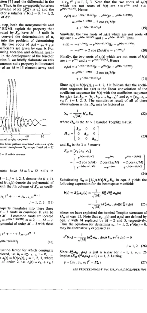
result. Note that the common nulls property is illustrated in Fig. 1 for the case of an M = 15 element array and

-

&nu, , i = 1, 2, as the two roots of q(z) = q,

+

qlz

1 6 r

spatial angle, degrees

Fig. 1 Plot of the respective beam pattern associated with each of the three columns of the M x 3 matrix beamjormer S, in eqn. 3 with M = 15 a n d u . = O

Note that the beams have M - 3 = 12 nulls in common __ reference beam

_ - _ _ upper auxiliary beam lower auxiliary beam

U, = 0; the three beams have M = 3 = 12 nulls in

common.

Let sij, i = 0,

..

., M - 1, j = 1, 2, 3, denote the (i

+

l), j component of S,, and let sJ{z) denote the polynomial of

order M - 1 formed with the jth column of S, as coeffi-

cients according to

S ~ ( Z ) = S o j + s , j z f s 2 j z ~ + " ' + S ~ - I , j Z ~ - ~ j = 1, 2, 3 (17)

The common nulls property translates into these three polynomials having M - 3 roots in common. It can be

shown [9, lo] that the M - 3 common roots are located

on the unit circle at z, =

P1u,+(2m/M)1,

m = 2,

.. .

, M - 2.

Let h(z) denote the polynomial of order M - 3 with these

roots:

h(z) = h,

+

hlz

+

hzz2

+

...

+

h M - 3 ~ M - 3

where aM is a normalisation factor for which conjugate

centrosymmetry is achieved, i.e. hi = h $ - 3 - i , i = 0,

. .

.,

M - 3. It follows that sJ{z) = h(z)e,(z), j = 1, 2, 3, where eiz) is a polynomial of order 2, i.e. eJ{z) = eOj

+

eljz 562

+

e2jz2, j = 1, 2, 3. Note that the two roots of s,(z)

which are not roots of h(z) are z = LP"~ and z = piu, +(Z/M)I, H~~~~

1

el(z) ~ e-jfflrk+(l/M)l(z -

@xZ

-

&nluc+(2/M)1

-

&xI*+(UM)l - 2 cos ( n / ~ ) z

+ e - j n l u ~ + ~ l / M ) l z 2 (19)

Since sJ{z) = h(z)e@), j = 1, 2, 3 it follows that the coeffi-

cient sequence for sJ{z) is the linear convolution of the

coefficient sequence for h(z) with the coefficient sequence

for e{z) Let 11, = [h,, h , , ..., hM-3]T and ej = [eoj, elj, ej2]< j ' = 1, 2, 3. The cumulative result of all of these. observations is that S, may be factored as

where H , is the M x 3 banded Toeplitz matrix

H M = r i

Substituting S, = [l/J(M)]HM E , in eqn. 8 yields the

following expression for the beamspace manifold:

where we have exploited the banded ToepEtz structure of

H , in eqn. 23. Note that a,_,(u) and a&) are defined by eqn. 2 with M replaced by M - 2 and 3, respectively.

Thus the equation for determing u t , i = 1, 2, uTb(ui) = 0, may be alternatively expressed as

i = 1, 2 (26)

Since l l ~ a M - Z ( ~ i ) is just a scalar for i = 1, 2, eqn. 26

implies (EMo)"a,(ui) = 0, i = 1,2. Letting

4 = c40 3 41, 42IT = E; U (27)

(5)

then eqn. 26 implies that ii = 8"',, i = 1, 2, are the two

roots of the second-order polynomial q(z) = qn

+

q,z

+

q 2 !2, where q2 = q:

.

It is easily verified that the pre- scription for the components of q in eqn. 27, where E, is defined by eqn. 24, is exactly the same as that in eqn. 6.

Symmetric: The final step in either version of the algorithm is to estimate z1 = and z 2 = $.y* as the two roots of q(z) = qo

+

qlz

+

q: z 2 . In the symmetric case, this final step may be simplified somewhat by exploiting the fact that u3 = U , in eqn. 6. In this case, the coefficients

of q(z) simplify as qn = e'xu~{v2 - 20, cos (n/M)} = q:

and q, = 40, cos ( n / M ) - 20, cos (2nlM). It is easily

shown that if

I

q!/qn

1

< 2, the two roots of q(z) lie on the unit circle equidistant from the point z = $.ye, Equating the phase angle of that root of q(z) having the larger phase angle with that of i, = 8"'' yields, after some alge- braic manipulation, the expression for ii, in eqn. 7. If

1

q l / q o

1 >

2, the direct and specular path signals are not

resolved.

3

In the case where U, = ug, B = [b(u,)

f

b(u2)] satisfies

r3

Br2 = B. This property gives meaning to the forward-

backward average in beamspace described by eqn. 14,

which in turn yields the effective source correlation matrix RC in eqn. 16. The bisector angle estimator to be

developed in this section is based on using

r3

Bf2 = B as

a discriminating feature between the case of U, = ug and the case of U, # us. Denote the signal-only (noise-free) component of Re {RL:} as Re

{Cl:}.

Specifically, the estimator is based on the fact that if U, = us then Re

{Cl:}

is of rank two and has a zero determinant, while if U, # us then Re {Ci:} is of full rank and has a nonzero determinant provided AY is not equal to either 0" or 180". The anomaly occurring with either AY = 0" or AY = 180" is averted by employing spatial smoothing [ll, 121.

In accordance with eqn. 15 Re

{Cl:},

as defined above, may be expressed as

Re

{Cl:}

= f { B Re {R,,}BT

+

r3

B Re {R,,}BTr3} (28)

Note that Re

{Cl:}

is a nonnegative-definite symmetric matrix. In the case U, = ug, Re

{Cl:}

simplifies as

B R i b B T , where RAb is defined by eqn. 16, owing to the

property

r,

BIZ = B. Since RAb is 2 x 2, it follows that

det (Re {Cl:}) = 0 in the case U, = ug

.

In contrast, in the case U, # ug eqn. 28 cannot be simplified further such

that

Estimation of the bisector angle

where we have assumed that AY is not equal to either 0" or 180" so that Re { R = } is of full rank. Note that, in accordance with eqn. 13, r3b(u,) = 4 2 4 - U,) and

r3

b(uJ = 4214 - uz). From the definition of b(u) in eqn.

8, it is easily proved that any three members of the set of four vectors {Mu,),

Nuz),

b(2u, - U,), b ( h , - u2)} are lin-

early independent provided uz # 2uc - U,, as would be the case when U, = uB. Thus Re

{Cl:}

is of full rank such that det (Re

{Cl:})

> 0 in the case U, # uB as long as AY is neither 0" nor 180". When AY is equal to either 0" to 180", Re {R,,} is of rank one such that the rank of Re

{Cl:}

is one as well and det (Re {Cl:}) = 0, as in the case U, = us. Thus, provided Re {R,,} is of full rank,

det (Re

{Cl:})

may be used to discriminate between the case U, = ug and the case U, # ug

.

IEE PROCEEDINGS-F, Vol. 138, N o . 6 , DECEMBER 1991

Spatial smoothing [ll, 121 is employed to obtain an

effective source correlation matrix that is of full rank regardless of the value of AY. In spatial smoothing, the beamspace sample correlation matrix is spatially averaged over a number of identical, overlapping subarrays. The procedure exploits the fact that the relative phase difference between the direct and specular signals at the centre of each subarray is different. We point out that spatial smoothing need only be employed in the process of estimating the bisector angle. Once this is accom- plished, one may estimate the arrival angle of the direct path signal via the symmetric version of the BDML algorithm outlined previously with U, equal to the bisector angle estimate. A negative side effect of spatial smoothing is that the effective aperture is that of the subarray. Although the reduction in the effective array aperture is not critical in the estimation of the bisector angle, the corresponding loss in resolution may prove critical in the subsequent estimation of the arrival angles of the direct and specular path signals.

The subarrays employed in spatial smoothing are each composed of L continuous elements, with adjacent sub- arrays having all but one element in common. An M element array is composed of M - L

+

1 such subarrays. The extraction of the L x 1 snapshot vector for the kth

subarray, denoted x,(n; k), k = 1,

...,

M - L

+

1, from

x(n) may be described mathematically as x , ( n ; k ) = J f x ( n ) n = I,

...,

N where ( k - 1 ) x L Jk=[:] L x L 0 ( M - L - k + + ) x L k = 1, ..., M - L

+

1 (30)

With these subarray snapshot vectors, the spatially smoothed element space correlation matrix, denoted

a,,

,

is constructed as

Finally, the spatially smoothed beamspace sample correlation matrix, denoted

ab,,

is formed as

(32)

@bb =

sf

'Xx ' L

where

Here uL(u) is described by eqn. 2 with M replaced by L. It

can be shown 1 1 , 121 that the signal-only (noise-free)

component of

Lb,

denoted

ebb,

may be expressed as where B, = [ S f u L ( u l ) Sfa,(u,)] = [bs(ul) bs(u2)] and

a,,

is the effective source correlation matrix

ebb = B8ass B f (34)

where

e - J = u ~

@ =

[

0

e-e.]

From the theory espoused in that

a,,

is of full rank equal

(35) Ell], it is readily deduced

to two as long as u2 # U, 563

(6)

and M - L

+

1 2 2. In the case under consideration,

however, the difference between u1 and u2 is quite small such that Re

{as}

may be ill-conditioned in the case of either AY = 0" or AY = 180". Simulations have indi-

cated that L = (2/3)M is adequate for angular separa-

tions between the direct and specular paths as small as a tenth of a beamwidth.

abb

has the asymptotic form

E{@,,} = B s a , B f + a i I , (36)

such that the smallest eigenvalue of E { a , , } , denoted I.:",

is G.'. e b b may thus be estimated

eb

-

a,,,

- 1 3 ,

where

1%"

is the smallest eigenvalue of

h,;.

Correspond- ingly,

e{:

may be estimated as

e{:

= * { a b ,

+

I3 a b b f3} -

2;:"

I 3 (37)

From the arguments provided previously, it follows that in the asymptotic/noise case, det (Re

{e{:})

>, 0 when U, # us regardless of the value of AY, while det (Re

{e{:})

= 0 when U, = us. This observation prompts the scheme for estimating the bisector angle us described below.

Consider U, in the definition of S, in eqn. 33 to be a

variable quantity. To emphasise such, we will alternatively denote

s,

as

s,(~,).

This dictates that

abb

and

cl:

computed according to eqns. 32 and 37, respectively, are

functions of U as well and should be alternatively denoted as a',,(u,) and

e{:(u,),

respectively. Given

e{&),

the bisector angle may be estimated as that value of U, in the vicinity of broadside for which det (Re { ~ { ~ ( U J } ) achieves its minimum value. Note that

in terms of the spatially smoothed element space correlation matrix

a,,

constructed according to eqn. 31,

Re {R{,b(u,)} may be expressed as

Re {'bb('c)} = Re {sF(uc)axx sL('c)}

= t ~ s ~ ( u , ) ~ x , ~ L ( u , )

=

sF(~,)~::s,(u,)

(38)

+

sZ(uc)rN I N

a:;

b

r N S ? ( U c ) }

where

a::

is the forward-backward-averaged element space sample correlation matrix [12]

a::

=

${a,,

+

.?Nk:x&} (39)

Hence, the bisector angle estimation procedure described above may be formulated as

minimise det (+{$'(uJei: SL(u,)

+

I 3

sF(%)e::

s L ( U J r 3 H (40)

where

e::

= - 6 i l N and 8: is an estimate of the noise power. That is, the bisector angle estimate is that value of U, which minimises the objective function in eqn. 40. Given an upper and a lower limit on the estimate of

the bisector angle, a 1-D search procedure such as golden

section search may be used to determine the minimising value of U,, Note that 5: may be estimated as the smal-

lest eigenvalue of Rbb(u,) (or Re {~,,(u,)}) for any value of U, in the vicinity of broadside.

The bisector angle estimation procedure described by eqn. 40 is not a closed-form procedure but requires a 1-D

search. However, a simple closed-form estimation procedure may be obtained by factoring

s,(~,)

similar t o

eqn. 22. Exploitation of this factorisation allows us to formulate the search for minimising U, in eqn. 40 in terms

of finding I , = ej"". as the root of a quartic equation. The appropriate development is provided below.

564

Note that SL(uc) may be factored similar to eqn. 22 as

~ A U , ) = HL(u,)EL(uJ (41)

J(L)

where H,(u,) and E,@,) are defined by eqns. 23 and 24,

respectively, with M replaced by L and the dependence

on U, explicitly indicated. Specifically, HL(u,) is the L x 3

banded Toeplitz matrix

hL(%) 0 H L ( U J =

[

0"

]

(42) W(u,) =

[

0"

1

0"

]

[:

:

3

h L ( U , )

where hL(u,) is the ( L

-

2) x 1 coefficient vector for the common roots polynomial defined similar to h(z) in eqn. 18 but with M replaced by L and the dependence on U,

explicitly indicated. Also, note that E,(u,) may be fac-

tored as

E L ( U J = W(u,)E,(O) (43)

where EL(0) is defined by eqn. 24 with M replaced by L

and U, = 0 and

0 0

or

W(A,) = 0 1 0 where A, =

e

(44)

Substitution of .!?,(U,) = [l/~(L)]H,(u,)W(u,)E,(O) in the objective function in eqn. 40 yields, after some manipula-

tion and dropping the factor [l/J(L)],

det O{SF(~,)~if:s,(u,)

+ &

**W4,)e~:*st(~Jr~))**

= det ( E f ( 0 ) Re { W*(u,)HF(u,)

x H,(u,)WuJIE,(O))

x

e::

HL(UC)W(4J) det (EL(0)) = det (EF(0)) det (Re { W*(u,)HF(u,)

(45)

where we have invoked the following properties:

SF(u,)C:: S,(u,) is real-valued,

r3

E,(O) = EZ(O), and

det ( A B ) = det ( A ) det (B) if A and B are both square.

Since det (E,(O)) does not depend on U,, we may refor- mulate the optimisation problem in eqn. 40 as

minimise det (Re { W*(uc)H?(uc)e:: HL(u,) W(u,)}) (46)

This does not simplify matters very much owing to the U,

dependence in H,(u,). We now argue that this depen-

dence is inconsequential as long as U, is in the vicinity of the actual arrival angles such that we may replace HL(u,)

in eqn. 46 by HL(0). This assumes arrivals near broadside, as would be the case in an actual low-angle radar tracking scenario. This simplification facilitates simple closed- form solution for U,. The supporting argument is as follows.

Consider the asymptotic/noiseless form of the objective function in eqn. 46. To this end, note that the

asymptotic/noiseless form of

e::

may be expressed as

e::

= A , Re { a , } A F (47)

(7)

where A, = [aL(ul)

!

a,(u2)]. Substitution of eqn. 47 in

eqn. 46 yields, after some manipulation,

det (Re { W * ( u , ) H ~ ( u , ) c ~ : H , ( u , ) W ( u , ) } )

= det (Re { W*(u,)A3 G(u,) Re {fi,}C*(u,)A 'j W(u,)}) (48)

where A, = [a3(ul)

!

a3(u2)] and

C(u,)

is the 2 x 2 diago-

nal matrix

(49)

The expression on the RHS of eqn. 48 follows from the

banded Toeplitz structure of HL(uC) similar to the result in eqn. 25. Recall that what we desire is that the determi-

nant in eqn. 48 be zero when U, is equal to the bisector angle, uE = {ul

+

u2}/2, and strictly positive (nonzero)

otherwise. For this to be the case, we need only require in eqn. 48 that G(uJ in eqn. 49 be of full rank equal to two.

Assuming the arrival angles to be in the vicinity of broadside (U, = 0), this requirement will certainly be satisfied if we replace HL(uc) by H,(O) in eqn. 48.

To substantiate this claim and provide insight into the estimation scheme, note that

e-irr(ui -U<) e - j f f ( u z - u , l

p ( " l - * )

p,("l-",)

When U, = U, = {U'

+

u2}/2, { W*(uB)!3}4

from which we deduce, exploiting the 'tnck'

7

r(u,)AS, - 1 2 , Re { W * ( u E ) A 3

c(o)

Re _'j_{W ( u B ) }}

= W * ( u L ? ) A 3 f { G ( o ) Re { B s s ) G * ( o )

which has rank 2 and determinant zero as required as

long as G(0) is of full rank. When U, # U,,

{ W*(uE)A 3 } r 2 # W(uE)A: such that Re { W*(u,)A C(0)

Re { ~ , , } C * ( O ) A ~ W ( u , ) } is of full rank and, as a consequence, has a strictly positive (nonzero) determinant. This demonstrates the efficacy of the estimation procedure and substantiates the claim that this efficacy is not altered by replacing HL(u,) by H,(O) in the objective function in eqn. 46.

Based on these observations, the bisector angle estimate ic, is that U, satisfying

minimise det (Re { W*(u,)c{l W(u,)}) (52)

where

cif,"

= HF(O))C$H,(O). Note that since S,(O) =

(l/JL)H,(O)E,(O), it follows that H,(O) =

(JL)S,(O)E, '(0). Hence

where

abb

is constructed according to eqn. 32 with S, = S,(O) and

A::.,

is the smallest eigenvalue of

Rbb.

In the Appendix it is shown that the solution to the optimisation problem in eqn. 52 may be obtained by solving

for

1,

= &2"" as a root of the quartic polynomial

p(1) = -2pg - p:1+ p113

+

2p014 = 0 (54) IEE PROCEEDINGS-F, Vol. 138, No. 6, DECEMBER I991

where po and p1 are functions of the components of

e{:,

denoted (55) (56) i, j = 1, 2, 3 : P O = (c{j):2(ci(hb)13 - (clL)22(e{L):3 P i = 2

I(c{,"hb)~z

12(cli)i3

- 2(c{L)11(c%2

It is easily shown that at least two of the roots of p(1) in eqn. 54 lie on the unit circle. Thus

A,

= is that root of p(1) lying on the unit circle which minimises the objec- tive function in eqn. 52. A summary of the bisector angle

estimation procedure is delineated below.

3.1 Algorithmic summary of bisector angle estimator 1 Construct

abb

according to eqns. 30-33 with S, = S.(O). U\ I

2 Compute

e."

as the smallest eigenvalue of and

3 Form

A{:

= (Ef(O))-' Re {cL!}(E,(0))-l, where

form )CL: = (1 2){Rbb

+

I,

Rbbr3}

-

"

:

1

I ~ . E,(O) is defined by eqn. 24 with M = L and U, = 0.

-4 Root p(2) = - 2pg - p:,?

+

p1A3

+

2p,

R4

= 0, where p o and pl are defined in eqns. 55 and 56.

5 Then fiE = (l/jn) In (&), where

2,

is that root of p(1) having unity magnitude for which det (Re { W*(A,)c@ W(A,)}) is a minimum, where W(1,) is defined in eqn. 44.

3.2 Alternative algorithm

With the bisector angle estimate obtained from the procedure above, one may estimate the arrival angle of the direct path signal via the symmetric version of the BDML algorithm outlined previously with U, equal to the bisector angle estimate. As indicated previously, this mode of operation makes use of the full array aperture for maximum resolving power. No spatial smoothing is required since the symmetric form of BDML does not exhibit any breakdown phenomenon with respect to the relative phase difference, AY. However, this mode of operation requires that we reform three beams with new point angles after the bisector angle has been estimated using beams formed with S,(O). As an alternative, we briefly develop an equivalent procedure which works with

abb

formed according to eqns. 30-33 with S, =

S,(O). This method avoids reforming beams or computing any new beamspace sample correlation matrices, but has a reduced resolution capability owing to the smaller aperture of the subarray.

As a first step, we show that is possible to construct a Householder transformation matrix M satisfying

Ma3(ul) = a3(u2) that only depends on the bisector angle

uE

.

M may be expressed as M = I3 - 2wwH, where w is a

vector having unity magnitude proportional to a3(ul)

- u3(u2). Note that M is unitary and that

(1

a3(ul)l12 =

jja3(u2))j2. Defining 6u such that u l = uE

+

6u and u2 = us

-

6u,

e - j n ( u s + d u ) e-jn(uB-du)

- p3('2) =

[

]

-

[

]

e j , ( " B + 6") &.%("E - 6")

= 2j sin (6u)

[-;;I

(57)

Thus w = [1/\/(2)][-e-jffUE, 0, &j"""]', which fortuitously

only depends on U, as stated previously. It is easily veri-

fied that M = I3 - 2ww" satisfies Ma,(ul) = a,(u2) and For the remainder of this development, S,(O), HL(0) and E,(O) will be simply be denoted as S,, H, and

= a3(u1).

(8)

E L , respectively. Recall that bs(u) = SF aL(u) = [ l/J(L)] x E; HF aL(u) = [ l/J(L)](L: aL- ,(u))EFa3(u). Hence

(EF)-'b$(u) a a3(u), where a denotes 'proportional to'. It follows that

M(E%'bs(u~) a Ma3(U1) = %(uz) (EF)-'b3(U2) (58)

Hence

{EFM(e!-'}b,(u,) a bs(u2)

{EFM(G!-l}b,(u,) a b,(u,) (59)

and

Let

f

= EFM(E?)-', a 3 x 3 matrix. Note that

ff

= M 2 = I,. Also,

f

= E:

r3

7,

~ 7 ,

r3(EF)-I =

E;M*(E;)-l =

**f*,**

where we have exploited the conjugate centrosymmetry of the columns of E,. This observation implies that

f

is real-valued. Observing eqn. 59, it

follows that for the case where U, = 0 # u s ,

f =

EFM(EF)-l plays the same role that plays for the case U, = u s , I.e. fb3(ul) cc b,(u$ and %,(U,) a b,(u,).

Note, however, that although is equal to its own inverse, it is not symmetric. Thus

ff'

# 1 3 . This is in

contrast to the case with

r3,

which is both symmetric and equal to its own inverse.

Thus, in the case of U, = 0 # ua. U is comouted as a

generalised eigenvector of the matrix pencil -{Re {I?:!},

Q"}, where

db",

=

{dbb

+

fdbb

f 7 / 2 and Q b =

I

+

f p } / 2 . It is easily verified that

dii

fT

= Rb", and

two of the generalised eigenvectors of {Re

{db",},

Q*b}

satisfv f'u = U while the third satisfies f T u = -U. The Q tb

f

T - - Q t b . As a consequence, it is easily shown that

. ...-

desirdd U is that satisfying f T u = U associated with the smaller generalised eigenvalue. Thus, the arrival angles of the direct and specular path signals may be alternatively estimated via the following algorithm:

0 Given

CB.

Also,

d

employed in the bisector angle estimation scheme, i.e. f b b constructed according to eqns.

3C33 with S, = S,(O). -. .

1 With

iB,

form M =

t3

- ~ w w " , where w = [1/J(2)][ - e - j z G B , 0,

$no8lT.

2 With

f =

E f M ( E F ) - ' , where EL is defined by

eqn. 24 with M = L and U = 0 , form

db",

=

{Rbb

+

f&

~ ) / 2 and ~ t= b( I

+

i#f)/2.

3 Compute U = [U,, u2,'u3]' a s t h a t generalised eigen-

vector of {Re

{db",},

Qtb} satisfying f'u = U associated with the smaller generalised eigenvalue.

roots of q(z) = qo

+

q,z

+

4: z2, where

4 - - eJnUl and z 2 = &jnu2 are estimated as the two

1

4o = B n u , { u l & ( x / L ) - + U 3 e - j ( n / L )

41 = -2(u1

+

U J cos

(E)

+

2u, cos

($)

4 Computer simulations

Computer simulations were conducted to assess the performance of symmetric BDML employing the bisector angle estimation scheme developed in Section 3. The combined scheme of bisector angle estimation followed symmetric BDML is referred to as symmetrised BDML or simply S-BDML. The linear array employed was composed of M = 15 identical elements uniformly spaced by a half-wavelength such that the corresponding standard 3 dB beamwidth at broadside is roughly sin-'(2/ 16) = 7.16". The following parameters were common to all of the simulation runs: direct path angle = 2", spe-

cular path angle O2 = - l o , p = 0.9. AY was varied 566

between 0" and 180" in steps of 22.5". Note that the angular separation between the direct and specular path signals, 3", is roughly four-tenths of a beamwidth and that the bisector angle is 0.5". Subarrays composed of

L = 11 contiguous elements were employed for spatial smoothing purposes in the estimation of the bisector angle. The noise added to the sensor signals was Gauss- ian, spatially white, and uncorrelated with the received signal echoes. Finally, for each algorithm sample means (SMEANs) and sample standard deviations (STDDEVs) of the respective estimates of 01, 8, or Os were computed from the results of 100 independent trials.

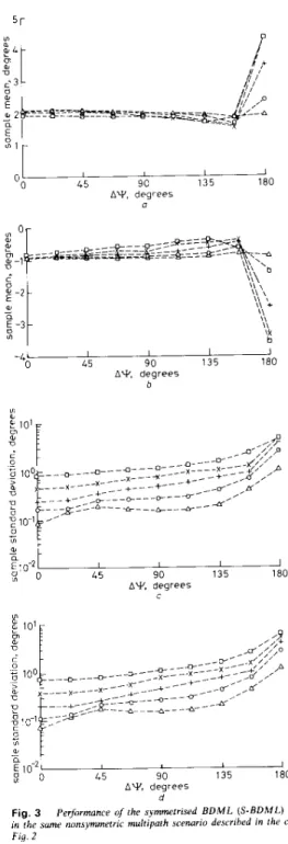
The simulation results presented in Figs. 2 and 3

compare the performance of nonsymmetric BDML with that of S-BDML given N = 5 snapshots for various com- binations of direct path SNR and AY. The breakdown of nonsymmetric BDML in the respective cases of AY = 0" and AY = 180" is evident in the results plotted in Fig. 2.

Nonsymmetric BDML simply does not provide reliable angle estimates for either of these two values of AY regardless of the SNR. The substantial improvement in performance achieved with S-BDML in the case of AY = 0" is exhibited in Fig. 2. The tradeoff for this improvement, of course, is the extra computation involved in computing the bisector angle estimate. The performance improvement in the case of AY = 90" is

rather modest as this value of AY is that for which nonsymmetric BDML performs best. Although S-BDML did not perform much better than nonsymmetric BDML in the case of AY = 180" for SNRs below 15 dB, reliable estimates were obtained with an SNR of 20 dB.

Fig. 4 displays the performance of the bisector angle

estimator employed in S-BDML for the simulations described above. A significant bias, roughly 0.05", is

observed with AY = 0" even at the relatively high SNR of 20 dB. Interestingly, the case of AY = 180" gave rise to the smallest bias in the bisector angle estimate for all SNR values except 0 dB. On the other hand, Fig. 3 indi- cates that the STDDEV of the corresponding S-BDML estimates of 8' and 8, were smallest in the case of AY = 0". In fact, although the respective Cramer-Rao lower bound (CRLB) is not plotted in Fig. 3c, the STDDEV of the S-BDML estimates of 8, for AY = 0" is significantly below the CRLB. The same is true with regard to the S-BDML estimates of 8,. This observation is, of course, not contradictory since the CRLB only holds for unbiased estimators. Furthermore, this observation substantiates the conjecture made in [5] that a

biased estimator must exist for which the performance in the case of AY = 0" is significantly better than that dictated by the CRLB.

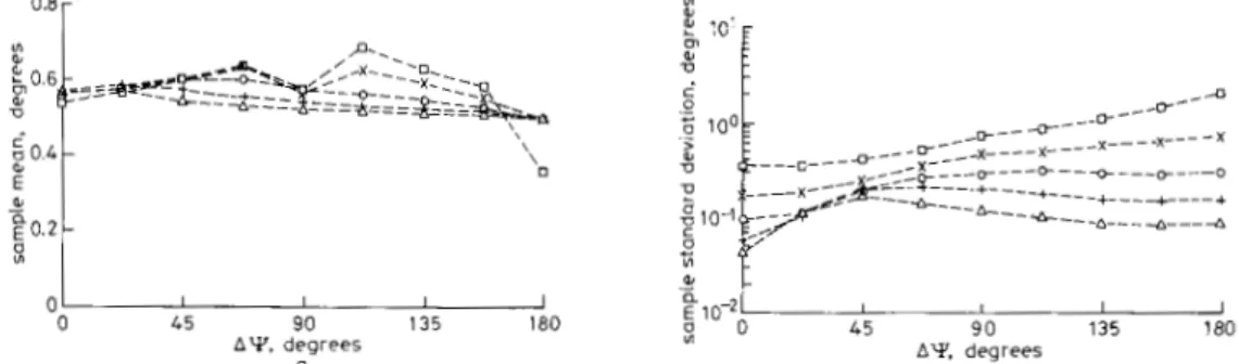
The second set of simulation results compares the performance and computational load of S-BDML with that of the improved three subaperture (3-APE) method of [ 6 ]

and the IQML method of [13]. The improved 3-APE method incorporates the practical constraint that the amplitude ratio p is less than one. The IQML algorithm is a computationally efficient implementation of the element space based ML estimation scheme. All simulation parameters were the same as in the first set of simulations discussed above except that the direct path SNR was fixed at 20 dB and each of the algorithms was exe-

cuted given only a single snapshot, i.e. N = I. SMEANs computed from estimates of the direct and specular path angles are plotted in Figs. 5a and 56, respectively. The corresponding STDDEVs are plotted in Figs. 5c and 5d along with the respective CRLBs. The CRLBs were computed based on formulas provided in [14].

(9)

The most important observation gleaned from Fig. 5 is that S-BDML significantly outperforms both 3-APE and IQML in the case of AY =

o",

and also in the case of

AY = 22.5". For example in Fig. 5d it is observed that

5r

I I I I 4 5 90 1 3 5 180 AYv degrees o b 0 I I I A T , degrees I 45 90 135 180 0 0 45 90 135 180 -1 0 A T * degrees b L5 90 135 180 $10 ' I A T , degrees m o C

Fig. 2 Performance o f t h r B D M L estimutor in a nonsymmetrlc multr- path scenario forfive different direct path S N R values

Target angle 0, = 2"; specular path angle 0 , = ~ 1 " ; M = 15: N = 5 and p = 0.9

Sample means and sample standard deviations were computed from 100 tndepen- dent rials

OOdB, x 5dB. + I0dB:O I5dB:AZOdB

n Direct path sample means

b Specular path sample means

c Direct path sample standard deviations

d Specular path sample standard deviations

I E E PROCEEDINGS-F, V o l . 138, N o . 6 , DECEMBER 1991 I I I J L5 9 0 135 180 -L 0 A V , degrees b I I I I L5 90 135 180 A T , degrees C 45 90 135 180 A T , degrees % O d

Fig. 3 Performance of the symmetrlsed B D M L ( S - B D M L ) estimator in the sume nonsymmetric multipath scenario described in the caption t o Fig. 2

OOdB: x 5dB:+ lOdB.Ol5dB;AZOdB

U Direct path sample means

h Specular path sample means

c Direct path sample standard deviations

d Specular path sample standard deviations

(10)

the STDDEV of the estimates of the specular path signal obtained from S-BDML for AY = 0" is approximately two orders of magnitude less than that obtained with either 3-APE or IQML. Observing the corresponding SMEANs plotted in Fig. 5b for AY = O", it is apparent that 3-APE and IQML simply provide unreliable estimates of the specular path angle for small values of AY.

0.8[

It should be noted, though, that the angle of interest is actually that of the direct path signal, The performance of 3-APE is much better in this regard; the STDDEV of the 3-APE estimates of the direct path angle for AY = 0" is below that dictated by the CRLB. The corresponding

bias, however, is rather high, approximately equal to -0.6". On the other hand, it is observed that the STDDEV

%

₅

_1o-Zo

F

,

l

VI 45 9 0 135 180

A Y * degrees b

Fig. 4 _{Performance of the bisector anale estimator}I n the .same nunsymmetric multipath scenario described in the caption tu Fig. 2 O O d B . x 5 d B ; O IOdB: + I S d B , A 2 o d B

a Sample means b Sample standard deviations

6 r O I

b

-5

t

1 o ' c I I I A Y , degrees I 4 5 9 0 1 3 5 180 d Fig. 5

Target angle 0, = 2 , specular path angle 8, = ~ 1 " . M = 15: N = 1; S N R = 20 dB for direct path; p = 0.9. Sample mean and sample standard deviation were computed from 100 independent trials

0 3-APE; x S-BDML: 0 IQML a Direct path sample means b Specular path sample means c Direcl path sample standard deviations d Specular path sample standard deviations

Comparison ufthe performance of S - B D M L with that oJ3-APE and I Q M L in a nonsymmetric multipath scenario

(11)

of the S-BDML estimates of the direct path angle for

A Y = 0" is below the CRLB by roughly an order of magnitude, while the bias is rather small, less than a tenth of a degree! IQML provides totally unreliable estimates of both angles in the case of A Y = 0". On the other hand, IQML significantly outperforms both S-BDML and 3-APE in the case of A Y = 180", achieving the CRLB.

To assess the tradeoff between performance and computational load among the three algorithms, the average number of floating point operations (flops) per execution was examined. This number was determined using the PRO-MATAB software package for each of the three algorithms under the conditions specified above; it did not include the initial computation involved in setting up the data. The numbers are: 3.8 x lo3 average number of

flops per execution for 3-APE, 7.4 x lo4 average number

of flops per execution for S-BDML, and 6.5 x lo5 average number of flops per execution for IQML. The respective numbers cited for both IQML and 3-APE are the respective averages obtained over all 900 trial runs (100 independent trials for each of nine different phase differences). In contrast to S-BDML, each of these two methods is iterative in nature, i.e. not closed-form. The actual number of flops for a given execution can vary rather significantly depending on the SNR and the value of A Y . Notwithstanding, note that the average computa-

tional load of 3-APE is roughly one-twentieth that of S-BDML and two orders of magnitude lower than that of IQML. The increased computational load of S-BDML relative to 3-APE is a tradeoff for the significant improvement in performance observed at the smaller values of

A Y . The algorithms perform similarly for A Y

>

45",

although the STDDEV curve for S-BDML was always lower than that for 3-APE. Finally, note that the computational load of S-BDML is roughly an order of magnitude lower than that of IQML.

5 Conclusions

In symmetrised BDML (S-BDML) the pointing angle of the centre beam is set equal to the bisector angle estimate, which is determined via a simple closed-form procedure. This facilitates a 'special' forward-backward average in beamspace which averts the breakdown of nonsymmetric BDML in the cases of A Y = 0" and

A Y = 180". Simulations indicate that in the case of

A Y = 0" the bisector angle estimator is biased but that the corresponding performance of S-BDML is significantly better than the CRLB. Simulations also indicate that S-BDML significantly outperforms improved 3-APE for values of A Y less than 22.5". The major difference in

computation between the two methods is in the initial steps: in 3-APE a beam is formed at each of three subarrays of M/3 elements involving 3(M/3) = M complex multiplications, while in S-BDML three beams are formed on the entire array involving 3M complex multiplications. Simulations also indicate that S-BDML sub- stantially outperforms IQML for values of A Y less than 22.5", while the opposite is true at A Y = 180". The performance of S-BDML in the case of A Y = 180" may be improved by employing the modified version developed at the end of Section 3, which works with a modified forward-backward average of the spatially smoothed beamspace sample correlation matrix employed in the bisector angle estimation scheme. However, the performance of this version of S-BDML in the case of

A Y = 0" is worse than that in which beams are reformed

IEE PROCEEDINGS-F, Vol. 138, No. 6 , DECEMBER 1991

using the entire array after bisector angle estimation. These observations, combined with the fact that nonsymmetric BDML performs comparably to S-BDML in the case of A Y = 90", motivate the development of a scheme for estimating A Y at the outset, which would then dictate

that version of BDML yielding the best combination of performance and computational load. Such an estimation scheme is currently under development.

6 Acknowledgments

This work was supported in part by the National Science Foundation under grant ECS-8707681, and by a grant from the Corporate Research and Development Center of the General Electric Company.

7 References

1 BARTON, D.K.: 'Low angle radar tracking', Proc. IEEE, 1974, 62,

pp. 687-704

2 WHITE, W.D.: 'Low angle radar tracking in the presence of multi- path', IEEE Trans., 1974, AES-10, pp. 835-853

3 GABRIEL, W.F.: 'A high-resolution target-tracking concept using spectral techniques'. NRL Technical Report 6109, May 1984 4 DAVIS, R.C., BRENNAN, L.E., and REED, L.S.: 'Angle estimation

with adantive arravs in external noise fields'. IEEE Trans.. AES-12, (3). pp. lis-186

.

5 CANTRELL, B.H, GORDON, W.B., and TRUNK, G.V.: 'Maximum likelihood elevation angle estimation of radar targets using subapertures', IEEE Trans., 1981, AES-17, (3), pp. 213-221 6 GORDON, W.B.: 'Improved three subaperture method for ele-

vation angle estimation', IEEE Trans., 1983, A B - 1 9 , (I), pp. 114-122

7 HAYKIN, S.: 'Radar array processing for angle of arrival estimation', in 'Array signal processing' (Prentice-Hall, Englewood Cliffs, NJ, 1985), Chapter 4

8 ZOLTOWSKI, M.: 'High resolution sensor array signal processing in the beamspace domain: novel techniques based on the poor resolution of Fourier beamforming'. Proceedings of the Fourth ASSP Workshop on Spectrum Estimation and Modeling, August 1988, pp. 35@355

9 LEE, T.S.: 'Beamspace domain M L based low-angle radar tracking with an array of antennas'. PhD Dissertation. Purdue University, December 1989

I O ZOLTOWSKI, M., and LEE, T.S.: 'Maximum likelihood based sensor array signal processing in the beamspace domain for low- angle radar tracking', IEEE Trans., 1991, SP-39, (3), pp. 656671 I 1 SHAN, T.J., WAX, M., and KAILATH, T.: 'On spatial smoothing

for direction-of-arrival estimation of coherent signals', IEEE Trans., 1985, A S P - 3 3 , pp. 806811

12 WILLIAMS, R.T., PRASAD, S., MAHALANABIS, A.K., and SIBUL, L.M.: 'An improved spatial smoothing technique for bearing estimation in a multipath environment', IEEE Trans., 1988, ASSP-36, pp. 42S432

13 BRESLER. Y., and MACOVSKI, A.: 'Exact maximum likelihood parameter estimation of superimposed exponential signals in noise',

IEEE Trans., 1986, ASSP-34, (9, pp. 1081-1089

14 STOICA, P., and NEHORAI, A.: 'MUSIC, maximum likelihood, and Cramer-Rao bound. Proceedings of the 1988 International Conference on Acoustics, Speech and Signal Processing, April 1988, pp. 22962299

8 AppendLx: converting det (Re

In this appendix we show that the cost function in eqn. 52 can be expressed in the form of a fourth-order polynomial and that the minimising ir, can be determined by rooting a quartic equation. We begin the derivation by substituting eqn. 44 into the matrix W*(uc)f?iL W(u,) in eqn. 52. Letting c i j denote the ijth component of

cl:,

i.e.

{ W * ( u , ) C i l , b ( u , ) } ) into a polynomial

(12)

Differentiating eqn. 62 with respect to U and setting to zero, we get

-2p,* e - 4 j n u c - p:e-2jw

+

ple2jKUc

+

2p0 e4jnuc = 0 (63) This suggests that the solution for U, can be obtained by solving the following quartic equation:

-2p,*1-2-p;r1 + p 1 1 + 2 p 0 1 2 = 0 (64) for a unit root I , , where

I,