國
立
交
通
大
學
電子工程學系 電子研究所
碩 士 論 文
認知無線網路:賽局模型與統計學習法之自我組織演算法
Cognitive Radio Networks: Game Modeling and
Self-organization Using Stochastic Learning
研 究 生:林震豪
指導教授:黃經堯 博士
認知無線網路:賽局模型與統計學習法之自我組織演算法
Cognitive Radio Networks: Game Modeling and
Self-organization Using Stochastic Learning
研究生:林震豪
Student: Chen-Hao Lin
指導教授: 黃經堯 博士
Advisor: Dr. ChingYao Huang
國
立 交 通 大 學
電子工程學系
電子研究所
碩
士 論 文
A Thesis
Submitted to Department of Electronics Engineering and Institute of Electronics
College of Electrical and Computer Engineering National Chiao Tung University
in partial Fulfillment of the Requirements for the Degree of
Master in
Electronics Engineering June 2013
Hsinchu, Taiwan, Republic of China
Cognitive Radio Networks: Game Modeling and
Self-organization Using Stochastic Learning
Student: Chen-Hao Lin
Advisor: Dr. ChingYao Huang
Department of electronics engineering
Institute of electronics
National Chiao Tung University
Abstract
Due to the high demand of spectrum utilization, cognitive radio (CR) network has been a promising solution to the problem of spectrum scarcity by using dynamic spectrum access technique. The CR networks is applied to the original network (or primary network) without modifying the original network. In this paper, we studied one of the CR network architectures, CR network access architecture, where the CR base stations (CRBSs) demand spectrum resources from the primary network and distribute them to the CR users. We applied an economical Cournot Game model to the system where the CRBSs are the players and compete for better performance in this game. In order to optimize the game, we proposed a stochastic learning (SL) based scheme for the CRBSs to adjust the demand amount of resources based only on the action-reward history, which means there is no need for a centralized controller. We proved that the SL-based algorithm leads the system to converge toward a Nash Equilibrium (NE) point. Numerical results correspond to the proof. The results also show that the system performs well in terms of the total utility comparing with other schemes.
認知無線網路:賽局模型與統計學習法之自我組織演算法
研究生:林震豪
指導教授: 黃經堯 博士
國立交通大學
電子工程研究所
摘要
為因應頻寬上的需求及使用效率,認知無線 (cognitive radio)技術已被視為 一可行且有效的解決方法,該技術能解決目前頻寬使用上的一大問題,也就是 頻寬使用的分散性,統計發現一般用戶並不會持續地使用該頻寬,造成頻寬上 的頻寬洞 (spectrum hole),頻寬使用率大幅降低,認知無線技術將認知無線 網路建構在已經存在的主網路上,偵測並且使用主網路的頻寬洞,本論文主要 研究認知無線網路的其中一個架構─認知無線網路通路 (CR network access architecture),該架構主要由一頻寬經濟人 (spectrum broker)蒐集認知無線 網路的資訊,進而分配頻寬資源給各個認知無線網路的認知無線基地台 (CR base station),認知無線基地台的用戶能從這些基地台使用主網路多餘的頻 寬,我們將該架構以一經濟學模型─古諾模型 (Cournot game model)來描述, 認知無線基地台對頻寬經濟人提出頻寬資源需求,但同時也必須考慮競爭者, 也就是其他的認知無線基地台,去評估需求大小,我們使用統計學習 (stochastic learning)演算法,調整每個認知無線基地台對頻寬經濟人所提出 的頻寬資源需求,此演算法的好處是認知無線基地台只需要自我回饋的資訊即 可調整頻寬需求大小,不需其他認知無線基地台或是通道環境等資訊,本論文 證明該演算法能夠使系統收斂至納許均衡點 (Nash equilibrium),實驗的結果 除了反映證明外,也顯示了該演算法在整體效用的表現上具有顯著的成效。 IIThanks
碩士班念了三年,終於要畢業了,回想這三年,學習到的東西很充實,也 很紮實,一路下來遇到了不少貴人,讓我能順利畢業。 首先我要感謝幫助我完成論文的曾理銓學長,他一路下來幫助我解決問 題、給予指導,並在關鍵時刻督促我及時投遞研討會論文,因為我們都有出國 留學歐洲的經驗,常聊到一些關於歐洲教育的話題,感謝他讓我對於事物的看 法有更多面向。 另外要感謝兩位博班的 Robert 和 Maria,在我碩二的時候,我們一起參加 微軟舉辦的 Imagine Cup 競賽,得到第二名的佳績,雖然每天都要熬夜到早上, 但過程是開心而且有成就感的,這次的比賽是我碩士最美好的回憶之一。 再來我要感謝黃經堯老師,老師對於我做的決定,不管是參加微軟競賽或是 碩三上的交換學生,都很支持,老師也在論文上適時給予建議,讓我能夠反思許 多沒有考慮過的問題,很感謝他。 最後我要感謝我的父母,在我念碩士的期間沒有經濟壓力,在碩三上交換學 生時期,更贊助我生活費,讓我不必為學費操心,專心於課業上的努力。 還有許多人無法在此一一感謝,謹以此篇畢業論文獻給大家。 林震豪 謹誌 2013 年 6 月, Wintech Lab, 交大, 新竹, 台灣 IIIContents
Abstract ... I 摘要 ... II Thanks ... III Contents ... IV List of Figures ... VI List of Tables ... VIIChapter 1 Introduction ... 1
1.1 Inefficient usage of the spectrum ... 1
1.2 Cognitive radio network ... 1
1.3 Cournot game ... 3
1.4 Stochastic learning ... 4
Chapter 2 System model and problem formulation ... 6
2.1 Game-theoretic model ... 8
2.2 Problem formulation ... 9
2.3 Analysis of Nash equilibrium ... 10
Chapter 3 Stochastic-learning-based algorithm design ... 12
3.1 Stochastic-learning-based algorithm ... 12
3.2 Analysis of self-organized channel number selection algorithm ... 13
Chapter 4 Simulation ... 17
4.1 Simulation 1 (M=3) ... 17
4.2 Simulation 2 (M=9) ... 18
Chapter 5 Results ... 19
5.1 The convergence behavior and Nash equilibrium point (M = 3)... 19
5.2 Utility performance (M = 3) ... 27
5.3 The convergence behavior and Nash equilibrium point (M = 9)... 28
5.4 Utility performance (M = 9) ... 35
Chapter 6 Conclusion ... 36 References ... 37
List of Figures
Fig. 1 Spectrum hole. ... 1
Fig. 2 Cognitive radio network architecture[2]. ... 2
Fig. 3 The overview of CR network access architecture. ... 7
Fig. 4 Probability evolution of the mixed strategies of CRBS1 (M=3). ... 19
Fig. 5 Probability evolution of the mixed strategies of CRBS2 (M=3). ... 20
Fig. 6 Probability evolution of the mixed strategies of CRBS3 (M=3). ... 20
Fig. 7 Probability evolution of the mixed strategies of CRBS4 (M=3). ... 21
Fig. 8 Probability evolution of the mixed strategies of CRBS5 (M=3). ... 21
Fig. 9 Probability evolution of the mixed strategies of CRBS6 (M=3). ... 22
Fig. 10 Probability evolution of the mixed strategies of CRBS7 (M=3). ... 22
Fig. 11 Probability evolution of the mixed strategies of CRBS8 (M=3). ... 23
Fig. 12 Probability evolution of the mixed strategies of CRBS9 (M=3). ... 23
Fig. 13 Probability evolution of the mixed strategies of CRBS10 (M=3). ... 24
Fig. 14 Test of unilateral deviation of each of the 10 players (M=3). ... 26
Fig. 15 Utility performance of SoCNS algorithm and other two schemes (M=3). ... 27
Fig. 16 Probability evolution of the mixed strategies of CRBS1 (M=9). ... 28
Fig. 17 Probability evolution of the mixed strategies of CRBS2 (M=9). ... 28
Fig. 18 Probability evolution of the mixed strategies of CRBS3 (M=9). ... 29
Fig. 19 Probability evolution of the mixed strategies of CRBS4 (M=9). ... 29
Fig. 20 Probability evolution of the mixed strategies of CRBS5 (M=9). ... 30
Fig. 21 Probability evolution of the mixed strategies of CRBS6 (M=9). ... 30
Fig. 22 Probability evolution of the mixed strategies of CRBS7 (M=9). ... 31
Fig. 23 Probability evolution of the mixed strategies of CRBS8 (M=9). ... 31
Fig. 24 Probability evolution of the mixed strategies of CRBS9 (M=9). ... 32
Fig. 25 Probability evolution of the mixed strategies of CRBS10 (M=9). ... 32
Fig. 26 Test of unilateral deviation of each of the 10 players (M=9). ... 34
List of Tables
Table 1 Symbols used in the modeling and system formultaion. ... 6
Table 2 Self-organized channel number selection. ... 13
Table 3 Parameters for Simulation 1. ... 18
Table 4 Parameters for Simulation 2. ... 18
Table 5 Records of the evolution process (M=3). ... 25
Table 6 Records of the evolution process (M=9). ... 33
Table 7 Utility performance of SoCNS algorithm and other two schemes (M=9). ... 35
Chapter 1 Introduction
1.1 Inefficient usage of the spectrum
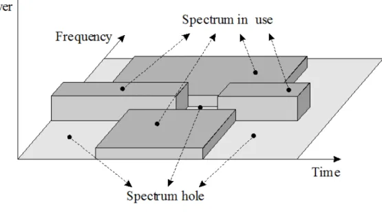
The demand of spectrum resources has been rapidly rising due to the increasing number of mobile device users. However the network has always been facing a problem of inefficient spectrum utilization. A spectrum owner (or primary user/service) subscribes to a band of a licensed spectrum. However the spectrum band is not always used and thus leaves holes in the spectrum, which causes inefficient usage of the spectrum. Fig. 1 describes the spectrum holes in the spectrum band. We can find out that spectrum holes appear in both time and frequency domain.
1.2 Cognitive radio network
In order to solve this problem, we applied cognitive radio (CR), which is defined as an intelligent wireless communication system that is aware of its environment and uses the
Fig. 1 Spectrum hole.
methodology of understanding-by-building to learn from the environment and to adapt to statistical variations in the input stimuli [1]. The CR network is imposed on the existing network without modifying the original network [2]. Utilizing the technique of dynamic spectrum access, the CR network is able to detect the unused spectrum bands [3] and distribute them to the CR users (or secondary users/services) who do not subscribe to the bands and have no permits to access the licensed spectrum resources. The CR network architecture is shown in the figure below.
In Fig. 2, we can discover that the CR users have three access types to use the spectrum resources, either directly or indirectly.
CR network access: The CR users access their own CR base station, on both licensed and unlicensed spectrum bands.
Fig. 2 Cognitive radio network architecture[2].
CR ad hoc access: CR users communicate with other CR users through an ad hoc connection on both licensed and unlicensed spectrum bands.
Primary network access: CR users can also access the primary base station through the licensed band directly.
In this paper, we studied the CR network access architecture. In this architecture, the CR users access their own CR base stations (CRBSs). Here a CRBS forms a CR network. As several CR networks share one common spectrum band, a spectrum broker [4] will collect the operation information from all the networks and distribute the resources properly to achieve efficient and fair spectrum sharing. The CR users can then access their own CRBSs and utilize the spectrum resources. The advantage of this architecture is that the CR network is independent of the original primary network and thus can have its own policy of spectrum sharing. In addition, there is only one hop interaction between the CRBSs and the CR users.
1.3 Cournot game
Game theory for cognitive radio networks has been studied recently since the emergence of CR network technology [5]. In traditional spectrum sharing, the network controller will face a lot of communication overhead when a small change of the network occurs. CR network, as a non-cooperative network, therefore requires game theory to model and solve its system.
Niyato and Hossain [6] have discussed the spectrum trading between the primary and secondary networks and considered the whole system as an economical model where the primary network is the spectrum supplier and the secondary network demands
spectrum resources. Gao et al. [7] have investigated an auction-based approach for dynamic spectrum access. The spectrum resources are priced and bid for by the secondary users. We formulated the CR network access architecture as a Cournot game (Cournot competition) [8], which is an economical game theory model.
Cournot game model originally describes the situation which more than one firm compete on the amount of the same product they will produce. All the firms decide independently and have no information of other firms' decision. However the price of the product is affected by the total amount of producing. The firms decide their own strategy and compete to maximize the profit. Both the efficiency and incentive issue need to be considered.
We considered the CRBSs as the players in the game. These players demand spectrum resources from the spectrum broker. The residual spectrum resources provided by the primary network are priced and the price is dependent on two factors, the external state and the players' behavior. The external state is the amount of residual spectrum resources provided by the primary network. The less the residual spectrum resources, the higher the price becomes. The second factor is the total demand from the CRBSs. The price increases with higher total demand. Since each CRBS acts as an individual and has no information of how many spectrum resources other CRBSs demand, the main issue of the game is how many spectrum resources each CRBS should demand from the spectrum broker in order to maximize the profit of itself and also the whole system.
1.4 Stochastic learning
We applied a stochastic learning (SL) solution for each CRBS to decide how much 4
amount of spectrum resources to demand and to adjust it according to the action-reward history. Many works [9]-[11] have studied SL in CR networks. However, they all focus on the architecture in which the CR users detect and utilize the residual spectrum resources directly from the primary network, where the channel selection is the main issue to be discussed. Our SL solution is with the following characteristics: (i) the CRBSs do not need to know the action of each other, (ii) the CRBSs do not have to know the availability of the residual spectrum resources. We proved that the SL-based algorithm converges toward a Nash Equilibrium (NE) point. Numerical results also show the convergence of the algorithm. We could also see that the algorithm performs quite well in the total utility comparing with two other schemes.
This paper is organized as follows. In Chapter 2, the system model for CR network access architecture is presented. We formulated the system as a Cournot game and proved that the model is an exact potential game (EPG), where the game possesses at least one Nash equilibrium (NE) point. Chapter 3 presents the SL procedure for each CRBSs. The proof shows that the SL procedure can make the system converge toward a NE point. The simulation settings are shown in Chapter 4. Finally, the numerical results are given in Chapter 5, followed by the conclusion drawn in Section Chapter 6.
Chapter 2 System model and problem formulation
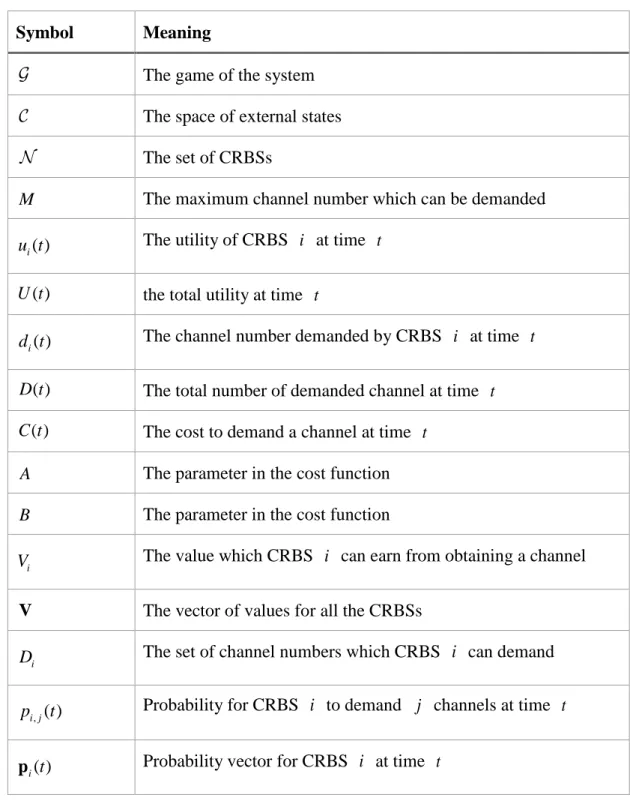
The symbols used in the modeling and problem formulation are summarized in Table 1.
Symbol Meaning
The game of the system The space of external states
The set of CRBSs
M The maximum channel number which can be demanded
( )
i
u t The utility of CRBS i at time t
( )
U t the total utility at time t
( )
i
d t The channel number demanded by CRBS i at time t
( )
D t The total number of demanded channel at time t
( )
C t The cost to demand a channel at time t
A The parameter in the cost function
B The parameter in the cost function
i
V The value which CRBS i can earn from obtaining a channel
V The vector of values for all the CRBSs
i
D The set of channel numbers which CRBS i can demand
, ( )
i j
p t Probability for CRBS i to demand j channels at time t
( )
i t
p Probability vector for CRBS i at time t
Table 1 Symbols used in the modeling and system formultaion. 6
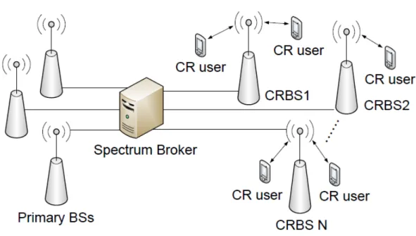
The CR network can be implemented for different scenarios [2]. In our work, we considered one of the CR network architectures, CR network access architecture, where the primary network gives out the residual channels to the spectrum broker, and the spectrum broker distributes the residual channels to the CRBSs according to their demands. Finally the CR users can utilize the spectrum resources from the CRBSs. The architecture is shown in Fig. 3. In our model, there are N CRBSs which serve
different numbers of CR users. CRBS i demands d t channels from the spectrum i( ) broker at time t. Each CRBS can demand at most M channels. Upon successfully
obtaining a channel, the CRBS-connected CR users can utilize the resources and benefit from sharing the residual channels.
On the other hand, the primary network gives out a number of residual channels. Note that the number of residual channels is time-varying with a fixed statistic character, and the CR network is not able to interfere with how many channels the primary network gives out. So when the primary network is fully occupied by the primary users, the
Fig. 3 The overview of CR network access architecture.
spectrum broker will detect no residual channels. The CR network then can never get any spectrum resources from the spectrum broker. In this situation, no matter how many channels the CRBSs demand, they are not allowed to share any resources with primary network. We will formulate this mechanism by an economical model in the next section.
To make the system more practical, we imposed the following assumptions.
The number of residual channels given out from the primary network is time varying. Its statistics are fixed but unknown to the CRBSs.
The system is decentralized which means the CRBSs have no information about how many channels other CRBSs demand. They act individually.
Notably, the only information available for decision making is the action-reward history of individual players.
2.1 Game-theoretic model
In this section, we present the game-theoretic formulation of the system. We considered the system as a Cournot Game (Cournot Competition) with external state. The players are the CRBSs. The game can be represented as a 4-tuple:
( , ,M u,{ }i i∈ )
=
where is the space of external states (number of residual channels), is the set of players, M is the maximum number of channels that a CRBS can demand, and
{ }ui i∈ is the utility function of player i that depends on his own decision as well as
the decisions of other players. The description of the utility function u is given below. i
At time t , CRBS i demand d channels from the spectrum broker. The cost i
( , )
C D t for demanding a channel depends on the total number of channels demanded
by all the CRBSs. In a typical Cournot Game model, the cost for demanding a channel is given by
1 ( , ) ( ) ( ), ( ) iN i( )
C D t = A t + ×B D t D t =
∑
= d t (1) where D t represents the total number of channels demanded by all the CRBSs at ( ) time t, B is a constant and A t is a parameter indicating the availability of the ( )residual channels at time t. In fact, A t increases while the number of the residual ( )
channels decreases in a linear fashion, which causes the cost to get higher. Note that ( )
A t changes with time since the number of the residual channels is time-varying with
a fixed statistic character which is not known by the CRBSs.
On the other hand, each CRBS benefits from successfully obtaining a channel from the spectrum broker. CRBS i earns a value V when a channel is obtained. The value i V i
depends on how many CR users are under the CRBS's service. We could then formulate the utility function u for CRBS i i as
( , ) ( ), 1, 2,...,
i i i i i
u d d− = ×d V −C i∈ N. (2)
And the total utility U is given by
1 N i i U =
∑
=u . (3)2.2 Problem formulation
The objective for each CRBS is to decide how many channels d to demand in order i
to maximize its utility u . Each CRBS desires to demand more channels to obtain a i
higher utility value for itself. However the cost C increases when the total demand 9
increases, which will decrease the value of Vi− and thus decrease the utility. Since C
the CRBSs have no information of each other's decision, they need to compete for their own benefit. Formally,
( ) : max ( , ),
i i
d∈ u d di i −i ∀ ∈i
(4)
2.3 Analysis of Nash equilibrium
With the utility function defined in (2), we show the existence of the NE point for the proposed Cournot game model in the following proposition.
Proposition 1. The game is an exact potential game (EPG) which possesses at least
one pure strategy Nash equilibrium (NE).
Proof: From the cost equation (1) and the utility function (2), we considered the function
1
: N +
Φ × × → for the game : 2 1 1 1 1 1 ( ,..., ) N N N N N i i i i i l i i i i l N d d V d A d B d B d d = = = < Φ =
∑
−∑
−∑
−∑
. (5)Note that the function Φ is a function of d1,...,d . Any change of N d1,...,d can N
affect the performance of Φ.
When CRBS i decides to demand another number of channels and changes its
strategy from d to i di′, the utility function will also change from u d di( ,i −i) to ( , )
i i i
u d d′ − .
It can be readily verified that
( , ) ( , ) ( , ) ( , )
i i i i i i i i i i
u d d′ − −u d d− = Φ d d′ − − Φ d d− (6) 10
As shown in (6), if the unilateral change of the strategy d can increase the utility i u , i
the increased utility will contribute the exact amount of improvement to the function
Φ. Therefore, as the players compete for better unilateral utility, they also benefit the total system.
Note that if q is a pure strategy NE, it must satisfy * ( *, *) ( , *),
i i i i i i i
u q q− ≥u q q− ∀ ≤q M
( *,qi q−i*) ( ,q qi −i*)
⇒ Φ ≥ Φ . (7)
When Φ satisfies the condition in (6), Φ is called the potential function of the game , and the game is said to be an exact potential game (EPG) and the existence of pure strategy NE is always guaranteed. This pure strategy NE is also a local maximum of the potential function Φ. Thus, Proposition 1 is proved. ■
However, we should note two things about NE.
A NE point doesn't guarantee the global maximum of the potential function Φ. There could be more than just one NE point, and the number of NE points of
is difficult to be confirmed.
Chapter 3 Stochastic-learning-based algorithm design
In this section, we discuss how to find the NE via SL. Here we propose a SL-based algorithm for each CRBS to decide how many channels d to demand for itself. This i
algorithm is decentralized so that each CRBS acts individually. The CRBSs learn toward the equilibrium state according to their action-reward history.
To facilitate the SL-based channel number selection algorithm, we extended the channel number selection game into a mixed strategy form. Let
,1 ,
( ) [ ( ), , ( )] ,T
i t = pi t pi M t ∀ ∈i
p be the channel number selection probability vector for player i, where pi j, ( )t is the probability that player i selects to demand j channels at time t.
3.1 Stochastic-learning-based algorithm
The proposed SL-based channel number selection algorithm is described in Table 2. In each time slot, each CRBS demands a number of channels according to the channel number selection probability vector. At the end of the time slot, a player obtains feedback from the competitive nature and updates the channel number selection probability vector p . The instantaneous reward serves as a reinforcement signal so i
that a high reward brings a high probability in the next time slot. Notably, the proposed learning algorithm is fully distributed: the channel number selection is solely based on the individual action-reward history, instead of the guide from a centralized controller.
Self-organized channel number selection (SoCNS) algorithm
1. Set t= , and the initial channel number selection probability vector as 0
, ( ) 1 / , ,
i j i
p t = M ∀ ∈i j∈.
2. At the beginning of each time slot, each player selects a number of channels to demand d t according to the current channel number selection probability i( ) vector pi( )t .
3. In each time slot, the cost C t will be evaluated and so will the utility ( ) u t i( ) specified by(2).
4. All CRBSs update their channel number selection probability vectors according to the following rules:
, , , , , , ( 1) ( ) ( )(1 ( )), ( ) ( 1) ( ) ( ) ( ), ( ) i j i j i i j i i j i j i i j i p t p t bu t p t j d t p t p t bu t p t j d t + = + − = + = − ≠ (8)
where 0< < is the learning rate. b 1
3.2 Analysis of self-organized channel number selection algorithm
In this section, we proved that the SoCNS algorithm can make our system converge to a pore NE point. To prove the convergence of the system, we first used the ordinary differential equation (ODE) to characterize the long-term behavior of the sequence {P( )t }, where P( )t =( ( ),...,P1 t PN( ))t is the mixed strategy channel number selectionprobability matrix. Secondly, we established a sufficient condition to achieve NE points for the SoCNS algorithm and proved that our system satisfies this condition.
Table 2 Self-organized channel number selection.
Proposition 2. With sufficiently small learning rate b , the sequence {P( )t } converges to P , which is the solution of the following ODE: *
0 ( ), (0) d F dt = = P P P P , (9)
where P is the initial mixed strategy channel number selection probability matrix and 0
( )
F P is the conditional expected function defined as:
( ) [ ( 1) | ( )]
F P =E P t+ P t . (10)
Note that P(t+1) follows that updating rule in (8).
Proof: Refer to Theorem 3.1 in [12]. ■
Proposition 3. The following are tru of the SL-based algorithm:
(1) All the stable stationary points of (9) are the Nash equilibria of . (2) All the Nash equilibria of are the stable stationary points of (9).
Proof: Refer to Theorem 3.2 in [12]. ■
Proposition 4. Suppose that there is a non-negative function H( ) :P P→R for some positive constant c such that:
' ' ' ( , ) ( , ) [ ( ) ( )], , , , i i i i i i id i i id H d H d c h h i d d − − − = − ∀ P P P P P (11)
where H d( ,P−i) is the value of H on the condition that pi is a unit vector with
the d th component unity, and hid( )P is the expected value of the utility of player
i where player i choose the strategy to demand d channels (i.e. di = ). d
( ) id h P is represented as following: 1 1 1 , ( ) [ ( ,..., , , ,..., ) ] k k id i i i N kd d k i k i h u d d− d d+ d p ≠ ≠ = ∑ ∏ P (12)
where the utility function ( ,u d di i −i) is defined in (2). 14
Then, the SL-based algorithm converges to a pore stragy NE point of the game.
Proof: We can re-write the ODE specified in (9) as following:
( ), ,1 id id dp qF i d M dt = P ∀ ∈ ≤ ≤ (13) Applying (8) and (10), (13) can be further derived into
1, max ( (1 ) [ | ( , )] ( ) [ | ( , )]) M id id id i i ik id i i k k i dp q p p u d p p u k dt = R − E P− + ∑= ≠ − E P− 1 max ( [ ( ) ( )]) M id ik id ik k qp p h h R = = ∑ P − P . (14)
It known that the variation of H P( ) is given by ( ) ( , i) id H H d p − ∂ = ∂ P P , (15)
where we use the fact that
1 ( ) ( , ) M id i d H p H d − = = ∑ P P .
With (11), (14) and (15), we can derive the derivation of H P( ) as following: , ( ) ( ) id i d id dp dH H dt p dt ∂ = ∑ ∂ P P , 1 max ( , ) ( [ ( ) ( )]) M id i id id ik i d k qp H d p h h R − = = ∑ P ∑ P − P , , max ( , i) id ik[ id( ) ik( )]) i d k q H d p p h h R − = ∑ P P − P , , max ( , , , ) 2 i d k i q Y i d k R − = ∑ P 2 , , max [ ( ) ( )] 0 id ik id ik i d k d qc p p h h R > = ∑ P − P ≥ , (16)
where Y = p p H did ik[ ( ,P−i)−H k( ,P−i)][hid( )P −hik( )]P . From (16), (14) and (13), we
can know ( ) 0 dH dt = P [ ( ) ( )] 0, , , id ik id ik p p h h i d k ⇒ P − P = ∀ ( ) 0, , id F i d ⇒ P = ∀
⇒ P is the stationary point of (9) (17)
In other words, the sequence {P( )t } converges to a stationary point of the ODE in (9). According to Proposition 3, Proposition 4 is proved. ■ Proposition 4 creates a sufficient condition that can guarantee the convergence towards NE. Next, we proved that our game satisfies this condition, which means the game
converges to a pure strategy NE point by applying the SoCNS algorithm.
Proposition 5. With sufficiently small learning rate b , the SoCNS algorithm
converges to a pure strategy NE for our game , which is an EPG.
Proof: Let H( )P = ΦE[ ( )]P , where Φ is the potential function defined by (5). Then
we will have: 1 1 1 , ( , ) [ ( ,..., , , ,..., ) ] k k i i i N kd d k i k i H d − d d− d d+ d p ≠ ≠ = ∑ Φ ∏ P . Applying (6) and (12), we can easily have:
'
'
( , i) ( , i) ( ) id( )
id
H d P− −H d P− =h P −h P
By proposition 4, proposition 5 is proved. ■
It is worth noticing that there is a trade-off for choosing the learning rate. A small learning rate implies slower convergence speed. However a large learning rate could lead to a serious accuracy problem. It is an important issue to choose the right learning rate and this rate can be determined by training in practice.
Chapter 4 Simulation
In this and next chapter, we evaluated the performance of the proposed algorithm. First of all, we needed to set up the parameters for the system.
4.1 Simulation 1 (M=3)
We considered the system with 10 CRBSs. Each CRBS can demand up to 3 channels in each time slot (i.e. M = 3). The parameters are defined in Table 3. Their value V i
for successfully obtaining a channel is given as a vector V=[ ,V V1 2,,VN]. Note that since we assume that each CRBS serves the same group of CR users in the whole learning process, the vector V is unchanged during the whole process. The parameter
A, which indicates the number of residual channels given out from the primary network,
is a Gaussian variable and changes with time slot. We set up different cases where the mean value of A, A equals from 1 to 10. A = 1 is the best case where there are many
residual channels given out from the primary network and A = 10 is the worst case where there are few residual channels.
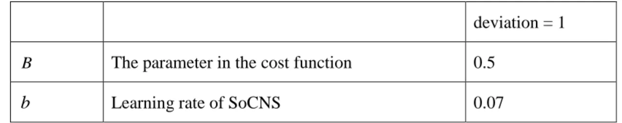
Parameter Description Assumption
| | Number of CRBSs 10
M Maximum channel number that a CRBS can
demand
3
V The vector of values that each CRBS can earn when successfully obtaining a channel
[12, 14, 11, 19, 20, 17, 12, 13, 18, 19] A The parameter in the cost function which
indicates the number of residual channels
Gaussian variable with mean = 1~10,
deviation = 1
B The parameter in the cost function 0.5
b Learning rate of SoCNS 0.07
4.2 Simulation 2 (M=9)
In the second simulation, we simply increased the maximum channel number, M,
which means that each CRBS has more choices to choose from. This can possibly increase the time for the CRBSs to converge and finally have a decision of how many residual channels to demand. The parameters are defined in Table 4.
Parameter Description Assumption
| | Number of CRBSs 10
M Maximum channel number that a CRBS can
demand
9
V The vector of values that each CRBS can earn when successfully obtaining a channel
[27, 29, 26, 34, 35, 32, 27, 28, 33, 34] A The parameter in the cost function which
indicates the number of residual channels
Gaussian variable with mean = 5 deviation = 1
B The parameter in the cost function 0.5
b Learning rate of SoCNS 0.05
Table 3 Parameters for Simulation 1.
Table 4 Parameters for Simulation 2.
Chapter 5 Results
The simulation results are divided in two parts. In the first part, we show the convergence of the SoCNS algorithm. We also show that the whole system converges to a NE point by testing unilateral deviation. In the second part, we compare the utility performance of the SoCNS algorithm with two other scenarios. One is exhaustive search, which considers a central controller that evaluates all the possible situations and chooses the best one. This can be seen as an upper bound of the performance. The other scenario is random selection where each CRBS chooses a channel number randomly. This is obviously the lower bound of the performance.
5.1 The convergence behavior and Nash equilibrium point (M = 3)
The following series of figure shows the evolution of the channel number selection probabilities while applying the SoCNS algorithm. In this case, we considered A as aGaussian variable with mean value 5, and deviation 1. The learning rate b of the
SoCNS algorithm is set 0.07.
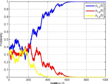
Fig. 4 Probability evolution of the mixed strategies of CRBS1 (M=3). 19
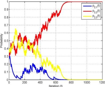
Fig. 6 Probability evolution of the mixed strategies of CRBS3 (M=3). Fig. 5 Probability evolution of the mixed strategies of CRBS2 (M=3).
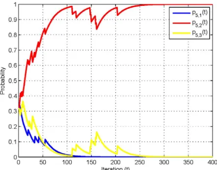
Fig. 8 Probability evolution of the mixed strategies of CRBS5 (M=3). Fig. 7 Probability evolution of the mixed strategies of CRBS4 (M=3).
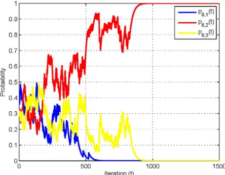
Fig. 10 Probability evolution of the mixed strategies of CRBS7 (M=3). Fig. 9 Probability evolution of the mixed strategies of CRBS6 (M=3).
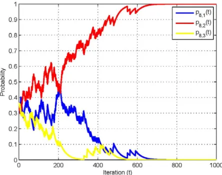
Fig. 12 Probability evolution of the mixed strategies of CRBS9 (M=3). Fig. 11 Probability evolution of the mixed strategies of CRBS8 (M=3).
Fig. 4 shows the probability evolution of CRBS 1. We could see the initial probability for each choice is the same. After about 600 time slots, it starts to converge and the final SL-based choice for CRBS 1 is to demand just 1 channel from the spectrum broker.
We observed another CRBS. Fig. 9 represents the probability evolution results for CRBS 6. The probabilities converge at around 900 time slots and the final SL-based choice for CRBS 6 is to demand 2 channels from the spectrum broker.
Fig. 5-8, 10-13 show the same convergence character as Fig. 4 and Fig. 9. Fig. 13 Probability evolution of the mixed strategies of CRBS10 (M=3).
Table 5 records important information of the evolution process for each CRBS. We recorded the point when the probability vector converges and the final decision. To judge the convergence point, we set the boundary 0.99, which means when the probability of a choice is greater the 0.99, we record that time slot.
CRBS Value V Convergence point (time slots) Final decision
1 12 601 1 2 14 737 2 3 11 572 1 4 19 526 3 5 20 246 2 6 17 904 2 7 12 488 1 8 13 650 2 9 18 1599 3 10 19 397 3
From Table 5, we could see that the whole system converges after 1599 time slots. And the final decision vector d=[1, 2,1, 3, 2, 2,1, 2, 3, 3].
Table 5 Records of the evolution process (M=3).
In Fig. 14(a), we test the unilateral deviation from the resulting strategy profile for all the CRBSs. The horizontal axis represents the cases of the 10 CRBSs. It can be observed that when one CRBS changes its strategy and chooses to demand a different channel number other than the original result, the unilateral utility would decrease. This shows that the resulting strategy profile converges toward a NE point. Fig. 14(b) shows the total utility deviation when one CRBS changes its strategy. We could see that there is no significant difference if only one CRBS diverts from its own strategy.
Fig. 14 Test of unilateral deviation of each of the 10 players (M=3).
5.2 Utility performance (M = 3)
In Fig. 15, we could see the performance of each channel number selection scheme. The horizontal axis represents the mean value of A which refers to the channel
availability and is dependent on the number of residual channels provided by the primary network. When A increases, the number of residual channels decreases,
which means there are less spectrum resources. We could see the total utility decreases as the spectrum resources decrease.
The exhaustive and random selection schemes clearly draw the upper bound and lower bound. The performance of SoCNS resides between the two bounds. Furthermore, we could observe that SoCNS performs quite well. It is closer to the upper bound and resides beyond around 80% from the lower bound.
Fig. 15 Utility performance of SoCNS algorithm and other two schemes (M=3).
5.3 The convergence behavior and Nash equilibrium point (M = 9)
In section 5.3 we expanded the choices form 3 to 9 for each CRBS. They can now demand up to 9 channels. In this case, we adjust the learning rate to 0.05, which is a bit less than the case of M=3 (0.07). Otherwise, the system doesn’t converge to a NE point (we could easily observe it by testing unilateral deviation). The following series of figure shows the probability evolution results.Fig. 17 Probability evolution of the mixed strategies of CRBS2 (M=9). Fig. 16 Probability evolution of the mixed strategies of CRBS1 (M=9).
Fig. 18 Probability evolution of the mixed strategies of CRBS3 (M=9).
Fig. 19 Probability evolution of the mixed strategies of CRBS4 (M=9).
Fig. 20 Probability evolution of the mixed strategies of CRBS5 (M=9).
Fig. 21 Probability evolution of the mixed strategies of CRBS6 (M=9).
Fig. 22 Probability evolution of the mixed strategies of CRBS7 (M=9).
Fig. 23 Probability evolution of the mixed strategies of CRBS8 (M=9).
Fig. 24 Probability evolution of the mixed strategies of CRBS9 (M=9).
Fig. 25 Probability evolution of the mixed strategies of CRBS10 (M=9).
Table 6 records important information of the evolution process for each CRBS.
CRBS Value V Convergence point (time slots) Final decision
1 12 1895 1 2 14 3775 1 3 11 2576 1 4 19 1636 9 5 20 706 6 6 17 3319 4 7 12 2054 5 8 13 4557 5 9 18 2754 8 10 19 2247 9
From Table 6, we could see that the whole system converges after 4557 time slots. And the final decision vector d=[1,1,1, 9, 6, 4, 5, 5,8, 9]. The time for the system to converge is much longer than the case of M=3 (1599 time slots), since there are more choices and the learning rate is decreased to 0.05.
Table 6 Records of the evolution process (M=9).
As in the simulation of the case of M=3, the test of unilateral deviation for the case of M=9 in Fig. 26 also shows that resulting strategy after SoCNS algorithm is a NE strategy, since as any one of the CRBSs changes its decision, its unilateral utility decreases.
Fig. 26 Test of unilateral deviation of each of the 10 players (M=9).
5.4 Utility performance (M = 9)
In this section, we considered the case when the mean value of A in (1) as 5 and the
variance as 1. Table 7 shows the resulting utility performance of each scheme. Scheme Utility
Exhaustive search 5.8744
SoCNS 5.5445
Random 4.9810
As we can see in Table 7, SoCNS can perform quite well on the utility. And there is one thing worth noticing. When we were doing the exhaustive search, we needed to consider all the possible combination of each CRBS. There are 10 CRBSs and each of them has 9 choices, so there are actually 9 strategies to evaluate, where the computation is 10 much heavier than SoCNS. Here if M =n, then the complexity is O n( 10), where our algorithm is O n , which increases linearly and relatively small. ( )
Table 7 Utility performance of SoCNS algorithm and other two schemes (M=9).
Chapter 6 Conclusion
We have studied the problem of self-organized channel number selection in one of the CR network architectures, CR network access, with time-varying channel and the absence of information of other CRBSs, by using a game-theoretic approach. The CR network access architecture is formulated as a Cournot game model where the CRBSs are the players in the game. The formulation is proved to be an EPG where at least one pure strategy NE exists. We have proposed a SL-based decentralized algorithm in which each CR user selects how many channels to demand according to its individual action-reward history. The algorithm has been proved to lead the system to converge to a pure NE in an EPG. The simulation results show the convergence character of the system. Also the unilateral deviation test shows the system converges toward a NE point. We also learn that there is no significant change if only one CRBS changes from its NE strategy.
References
[1] S. Haykin, “Cognitive radio: brain-empowered wireless communications”, Selected Areas in Communications, IEEE Journal on, vol. 23, no. 2, pp. 201–220, 2005.
[2] I. Akyildiz, W.-Y. Lee, M. C. Vuran, and S. Mohanty, “A survey on spectrum management in cognitive radio networks”, Communications Magazine, IEEE, vol. 46, no. 4, pp. 40–48, 2008.
[3] I. F. Akyildiz, W.-Y. Lee, M. C. Vuran, and S. Mohanty, “Next generation/dynamic spectrum access/cognitive radio wireless networks: a survey”, Computer Networks, vol. 50, no. 13, pp. 2127–2159, 2006.
[4] B. Wang and K.J.R. Liu, "Advances in Cognitive Radios: A Survey", IEEE Journal of Selected Topics on Signal Processing, special issue on Cooperative Communications and Signal Processing in Cognitive Radio Systems, vol 5, no 1, pp.5-23, Feb 2011.
[5] Beibei Wang, Yongle Wu, K.J. Ray Liu, “Game theory for cognitive radio networks: An overview”, Computer Networks, vol 54, no 14, pp.2537-2561, 2010. [6] D. Niyato and E. Hossain, “Spectrum trading in cognitive radio networks: A
market-equilibrium-based approach”, Wireless Communications, IEEE, vol. 15, no. 6, pp. 71–80, 2008.
[7] L. Gao, Y. Xu, and X. Wang, “Map: Multiauctioneer progressive auction for dynamic spectrum access”, Mobile Computing, IEEE Transactions on, vol. 10, no. 8, pp. 1144–1161, 2011.
[8] J. Watson, Strategy: An introduction to game theory. WW Norton, 2008.
[9] Y. Song, Y. Fang, and Y. Zhang, “Stochastic channel selection in cognitive radio 37
networks”, in Global Telecommunications Conference, 2007. GLOBECOM ’07. IEEE, 2007, pp. 4878–4882.
[10] Y. Xu, J. Wang, Q. Wu, A. Anpalagan, and Y.-D. Yao, “Opportunistic spectrum access in unknown dynamic environment: A game-theoretic stochastic learning solution”, Wireless Communications, IEEE Transactions on, vol. 11, no. 4, pp. 1380–1391, 2012.
[11] X. Zhou, Y. Li, Y. H. Kwon, and A. Soong, “Detection timing and channel selection for periodic spectrum sensing in cognitive radio”, in Global Telecommunications Conference, 2008. IEEE GLOBECOM 2008. IEEE, 2008, pp. 1–5.
[12] P. Sastry, V. Phansalkar, and M. Thathachar, “Decentralized learning of Nash equilibria in multi-person stochastic games with incomplete information”, IEEE Trans. Syst., Man, Cybern. B, vol. 24, no. 5, pp. 769-777, 1994.
![Fig. 2 Cognitive radio network architecture[2].](https://thumb-ap.123doks.com/thumbv2/9libinfo/8734923.202671/11.892.133.759.391.869/fig-cognitive-radio-network-architecture.webp)