適用於三維場景重建之寬基線立體影像匹配

國 立 交 通 大 學

電子工程學系 電子研究所碩士班

碩

士

論

文

適用於三維場景重建之

寬基線立體影像匹配

Wide-baseline Stereo Matching

for 3D Scene Reconstruction

研

究

生：劉彥廷

指 導 教 授：王聖智 教授

簡鳳村 教授

適用於三維場景重建之

寬基線立體影像匹配

Wide-baseline Stereo Matching

for 3D Scene Reconstruction

研 究 生：劉彥廷 Student：Yeng-Ting Liu

指 導 教 授：王聖智 教授 Advisor：Prof. Sheng-Jyh Wang

簡鳳村 教授 Prof. Feng-Tsun Chien

國 立 交 通 大 學

電子工程學系 電子研究所碩士班

碩 士 論 文

A Thesis

Submitted to Department of Electronics Engineering & Institute of Electronics College of Electrical and Computer Engineering

National Chiao Tung University in partial Fulfillment of the Requirements

for the Degree of Master of Science in

Electronics Engineering

September 2012

Hsinchu, Taiwan, Republic of China

i

適用於三維場景重建之

寬基線立體影像匹配

研究生：劉彥廷

指導教授：王聖智 教授

簡鳳村 教授

國立交通大學

電子工程學系 電子研究所碩士班

摘要

在本篇論文中，我們提出了可用於三維場景重建的寬基線立體影像對應系統。在 此系統中我們使用了三台未校準的相機，且這些相機被設置的很分散。由於大角 度所造成的扭曲和遮蔽的現象，使我們的匹配任務變得更加困難。 為了得到一 個準確的對應，我們採用了隨機森林來克服影像因大角度差而造成的扭曲，並使 用修改過的 Histogram of Oriented Gradients（HOG） 配合條件隨機場（CRF）來 求解，結合了這兩種方法不僅可修正錯誤的對應關係還可處理一些大角度遮蔽的 問題。 獲得匹配點以後，可經由 Bundle Adjustment（BA）求出世界座標點雲及 相機參數。接下來，我們加入了一個分割的方法(spectral matting)，讓我們可以根 據像素空間和色彩之間的關係來重新定義點雲的世界座標。 最後再根據點雲來 建立出一個立體的三維模型。

ii

Wide-baseline Stereo Matching

for 3D Scene Reconstruction

Student：Yeng-Ting Liu Advisor：Prof. Sheng-Jyh Wang

Prof. Feng-Tsun Chien

Department of Electronics Engineering, Institute of Electronics

National Chiao Tung University

Abstract

In this thesis, we present a wide-baseline stereo system for 3D scene reconstruction. We implement our system with multiple un-calibrated cameras which are set widely. The main challenge of the system lies on how to match image pairs at wide-baseline, in which there appear large perspective distortions and large occlusion areas between images. In this research, we attempt to tackle the problem based on machine learning and optimization techniques. In order to match image more accurately, we apply random forest to overcome large perspective distortions, and add Conditional Random Field (CRF) with modified Histogram of Oriented Gradients (HOG) to solve the matching problem. Combining conditional random field with random forest can not only correct error correspondences but handle some occlusions. After getting matched points, we use these correspondences to find a 3D point set and camera matric by bundle adjustment (BA) that minimizes re-projection error. Then, we use the idea of spectral matting to refine the 3D point set. Finally, we build a 3D model with the refined point set.

iii

致謝

感謝這兩年來帶領我做研究的兩位老師: 王聖智老師與 簡鳳村老師。 兩位 老師總是非常溫和的帶著我們做研究，儘管學生的資質再駑鈍，老師們都是很有 耐心的教導我們。讓我從完全不會上台報告，不懂如何讀書、整理重點到現在完 成碩士論文口試， 此過程中， 老師們不斷地糾正我，告訴我該如何報告、讀書、 找重點等等， 兩年來在老師們的教導下，非常有收穫！ 也要感謝實驗室的博班 學長: 信嘉、 敬群、 慈澄、 禎宇、 家豪，以及碩班學長: 維辰、 瑋國、 周 節、 育瑋、 韋弘、 玉書、 鄭綱、 郁霖、 開暘，學長們常回來分享他們過往 的研究經驗， 當我在研究之路上迷路時能指引方向，讓我能順利地走出來，還 能分享他們的工作經驗， 使我能提早對職場有進一步的了解，真的是非常的感 謝他們。 還有同屆的同學: 柏翔、 心憫、 耀笙、 秉修、 儲培、 利容，同學 們兩年來一起修課、數學訓練、進度報告、吃大餐、運動、玩樂等等，使我這兩 年的研究生涯過的非常歡樂又充實。 以及碩班的學弟妹們: 秉宸、 介暐、 姿 婷、 政銘、 佳峻，感謝學弟妹們在我口試時還能撥空幫忙買蛋糕飲料咖啡便當 等，真的是辛苦你們了。 還有台北台中的朋友們，當我研究碰到低潮時能給予 心情上的安慰與鼓勵，使我有動力能繼續向前。 真的非常高興能夠來到交大電 腦視覺實驗室學習， 這兩年認識了一群非常棒的朋友，希望未來大家能後繼續 聯絡、互助。

iv

Content

Chapter 1 Introduction ... 1

Chapter 2 Backgrounds ... 3

2.1 Local Approach ... 4

2.1.1 Appearance feature based method ... 4

2.1.2 Machine learning based method ... 8

2.2 Global Approach ... 9

Chapter 3 Proposed System ... 11

3.1 Keypoint Matching by Random Forest ... 12

3.1.1 Wide-baseline matching as a classification problem ... 13

3.1.2 Training the forest with random binary features ... 14

3.1.3 Feature selection ... 15

3.1.4 Keypoint classification ... 16

3.1.5 Matching results after random forest processing ... 18

3.2 Dense Matching by Conditional Random Field ... 18

3.2.1 Conditional random field (CRF) ... 18

3.2.2 Histograms of Orientated Gradients (HOG) ... 20

3.2.3 Modified HOG for distortion and occlusion handling ... 22

3.2.4 Matching points by MHOG with spatially constraint ... 24

3.2.5 Model formulation ... 26

3.3 3D Model Reconstruction ... 26

3.3.1 Camera calibration ... 26

3.3.2 Bundle adjustment ... 27

3.3.3 Random sample consensus (RANSAC) ... 28

3.3.4 3D point set refinement by matting refinement ... 29

3.4 Summary ... 32

Chapter 4 Experimental Results ... 34

4.1 Matching results... 34

4.1.1 Matching results by using random forest ... 34

4.1.2 Matching results after CRF correction ... 37

4.2 Reconstructed 3D models ... 40

Chapter 5 Conclusion ... 43

v

List of Figures

Figure 1-1 photo tourism: exploring photo collections in 3D [1] ... 2

Figure 2-1 (a) Image gradients (b) Keypoint descriptor (4 grids) [4] ... 5

Figure 2-2 SIFT matching result [4] ... 5

Figure 2-3 some keypoints detected by DoG in two views ... 6

Figure 2-4 SURF detector is an approximation of DOG [5] ... 6

Figure 2-5 SURF descriptor is a calculation of Haar wavelet [5] ... 7

Figure 2-6 (a) Detected region (b) Gradient image and location grids ... 8

Figure 2-7 top row: a reference patch horizontally scaled oblique view. Bottom row: other oblique views. [10] ... 9

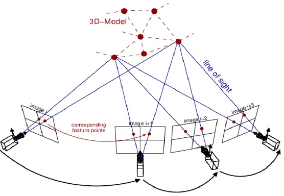
Figure 3-1 three-view stereo system [18] ... 11

Figure 3-2 Red region is occluded in the other view ... 12

Figure 3-3 Perspective distortion ... 12

Figure 3-4 Rotated patches ... 13

Figure 3-5 Randomize tree ... 14

Figure 3-6 (a), (b) are different trees’ separating results, different color represent different classes ... 16

Figure 3-7 Keypoints can be recognize by trained random forest ... 16

Figure 3-8 Matching result of random forest (Cleaner results are shown in Chapter 4.) ... 17

Figure 3-9 Some matches of Figure 3-8 ... 17

Figure 3-10 The same points matched by SIFT ... 17

Figure 3-11 3X3 neighborhood around a pixel ... 19

Figure 3-12 CRF model ... 20

Figure 3-13 HOG descriptor ... 21

Figure 3-14 Human’s HOG descriptor [20] ... 21

Figure 3-15 Modified HOG descriptor ... 22

Figure 3-16 Result comparison for different 𝛤 values ... 23

Figure 3-17 SIFT flow [21] ... 24

Figure 3-18 Matching result based on the CRF model ... 25

Figure 3-19 Camera geometry ... 27

Figure 3-20 Estimation of 3D points by using bundle adjustment... 28

Figure 3-21 (a) Data set with many outliers (b) Fitted line with RANSAC ... 29

Figure 3-22 (a) Locations of keypoints (b) Confidence map ... 30

Figure 3-23 Refined depth map (remove sky and ground) ... 31

vi

Figure 3-25 System flow ... 33

Figure 4-1Matched feature pairs by random forest ... 34

Figure 4-2 Some correct matches ... 35

Figure 4-3 Matched result by random forest (part1) ... 35

Figure 4-4 Matched result by random forest (part2) ... 35

Figure 4-5 Matching result of random forest ... 36

Figure 4-6 Result of CRF ... 37

Figure 4-7 Some matches of Figure 4-6 ... 37

Figure 4-8 Some matches of Figure 4-6 ... 37

Figure 4-9 SIFT result (many mismatched points over the region with repetitive patterns) ... 38

Figure 4-10 Some matched results of our system ... 38

Figure 4-11 Some matched results of our system ... 39

Figure 4-12 (a), (b), (c) Input images (d), (e), (f) Corresponding results of 3D reconstruction ... 40

Figure 4-13 Multi-view database “fountain” [7] ... 41

Figure 4-14 (a) Input images (b) Reconstructed 3D model ... 41

Figure 4-15 First row: short-baseline input images. Second row: reconstructed 3D models ... 42

vii

List of Tables

1

Chapter 1 Introduction

The task of finding correspondences between two or more images of the same scene or object is part of many computer vision applications, such as camera calibration, 3D reconstruction, image registration, and object recognition. In object recognition areas, researchers take many reference images that include target objects, and build these reference images in data base. Moreover, they can recognize target objects by matched correspondence result. In general, testing images may be taken from any viewpoints. That means, testing images will be distorted due to large perspective distortion and occlusion. In such cases, solutions for short baseline stereo matching cannot work well for wide baseline stereo. On the other hand, for pose estimation problems, it may be necessary to compute depth from two or more widely separated cameras, such as a surveillance application which may install cameras widely. Thus, wide baseline stereo matching problems become more important in recent years.

In 3D reconstruction areas, Microsoft developed a photo tourism system [1] in 2006 (shown in Figure 1-1) , by which users can explore photo collections in a 3D environment. They built a 3D virtual environment from photos collected from the internet. Many of the photos were taken from many viewpoints. Thus, matching these photos should rely on wide-baseline matchingtechniques. These examples reveal that wide baseline stereo matching problems become more important in recent years.

In the literature, quite a few work focus on finding correspondences by objects’ local gradient information so that the same object’s shape in different views might possibly be identified. However, objects shape will distort due to perspective

transform. Thus, some otherresearchers use machine learning approach to solve this problem.

2

(a) Photos from internet (b) 3D photos (c) 3D environment Figure 1-1 photo tourism: exploring photo collections in 3D [1]

In our 3D reconstruction system, likes many others. we first locate the interest points from training images using the method in DoG (Difference of Gaussian). Then the identified interest points are matched by means of the technique of the random forest [2]. Random forest is a machine learning approach that treats the matching problem as a classification problem.

Random forest can match interest points (keypoints) well, because random forest can naturally handles multiclass problems and it is robust and fast. In order to estimate 3D information, we need more point correspondences, which require larger memory capacity. So we first match the keypoints that have sufficient texture information (some regions with higher texture), and propagate these keypoints’ correspondences to neighbors by the CRF model. Therefore, our matching system requires less

memory capacity and gets more accurate result than the SIFT and random forest [3]. In this thesis, we will introduce some backgrounds in Chapter 2. Chapter 3 will present our proposed method for wide-baseline stereo matching technique,

experimental results are shown in Chapter 4, and we will give some conclusions in Chapter 5.

3

Chapter 2 Backgrounds

In the area of wide-baseline stereo matching, we can divide existing approaches into two branches. One is “Local” approach, many researchers try to find some

appropriate descriptors that are insensitive to light changes and perspective distortions, e.g. SIFT [4],SURF[5], GLOH [6] (Gradient location and orientation histogram). These approaches rely on counting the local gradient orientation histograms to

measure the similarity of pixels across images. But in wide baseline stereo, occlusions and perspective transformations become larger than short baseline stereo. Thus, wide baseline distortions will make these descriptors become weakly. In other words, appearance features (gradient, color …) can’t work very well because of serious distortions and occlusions. In recent years, some researchers [2, 3] proposed machine learning based method to recognize local deformed patches. In Section 2.1, we will introduce these local approaches in more details.

The other branch is “Global” approach. Traditional global approach favors simple pixel differencing, correlation over every small window [7]. They rely on optimization techniques, such as graph-cuts [8] to enforce spatial consistency. In addition, it is difficult to tune the window size in global the approaches, as a large window is tolerable to perspective variations and occlusions while a small window does not bring enough information.

Moreover, texture-less is another main challenge that needs to be handled using either a large window or a small window, due to that the texture-less regions do not contain enough information. The technique we proposed addresses both the

texture-less and occlusions issues. In our system, we designed a new descriptor to handle the occlusion areas, and we apply the CRF model to deal with texture-less regions.

4

2.1 Local Approach

In this section, we will introduce two kinds of local approaches, appearance feature based and machine learning based. In Section 2.1.1, we will introduce

appearance feature based method – SIFT, SURF and GLOH. In Section 2.1.2, we will introduce two machine learning based methods.

2.1.1 Appearance feature based method

The most common appearance feature based approach is Lowe’s method named Scale Invariant Feature Transform (SIFT) [4]. As SIFT transforms image into

scale-invariant coordinates relative to local features, it follows four stages to generate the set of image features:

The first stage searches over all scales and image locations. It is implemented efficiently by using a Difference of Gaussian (DoG) function which identifies potential interest points that are invariant to scale and orientation.

The second stage computes dominant orientation assigned to each keypoint location based on local image gradient directions. All future operations are computed on image data that has been transformed relative to the assigned dominant orientation, scale, and location for each feature, so they can provide invariance to these

transformations.

The third stage measures gradients at the selected scale in the region around each keypoint. These are transformed into a representation that allows for significant levels of local shape distortion and change in illumination. In Lowe’s implementation, the descriptor has 128 bins (16 grids and 8 orientations). As illustrated in Figure 2-1, it shows a part of grids.

5

(a) (b)

Figure 2-1 (a) Image gradients (b) Keypoint descriptor (4 grids) [4]

The final stage is finding the best candidate to match each keypoint which is found by identifying its nearest neighbor in the database of keypoints from images. The nearest neighbor is defined as the keypoint with minimum Euclidean distance for the invariant descriptor. That means, two points which have the nearest distance features are similar. Figure 2-2 shows a SIFT matching result.

Figure 2-2 SIFT matching result [4]

For image matching and recognition, SIFT features are extracted from a set of reference images and stored in a database. A new image is matched by comparing these SIFT features from the new image to this previous database and finding candidate matching. Thus, it can recognize the new image according to SIFT matching result. A big problem of SIFT is that SIFT features cannot separate

6

repetitive patterns well. In Figure 2-2, there are some similar corners that SIFT can’t recognize. Our system will overcome this problem.

Figure 2-3 some keypoints detected by DoG in two views

Bay, H. and Tuytelaars, T. perform Speeded up robust features (SURF) [5] for speed up computation time. The SURF detector is based on the Hessian matrix but uses a very basic approximation, just likes DoG which is a very basic Laplacian-based detector. It relies on integral images to reduce the computation time.

Figure 2-4 SURF detector is an approximation of DOG [5]

7

The SURF descriptor describes a distribution by Haar-wavelet responses within the interest point neighborhood. Again, they exploit integral images for speed up. Moreover, only 64 dimensions that include 4 x 4 square sub-regions and each

sub-region contain four features (dx, |dx|, dy, |dy| ), The lower dimensions are used to reduce the time for feature computation and matching.

Figure 2-5 SURF descriptor is a calculation of Haar wavelet [5]

Gradient location and orientation histogram (GLOH) is a new descriptor, which is an extension of the SIFT descriptor. It is designed to increase its robustness. They compute the SIFT descriptor for a log-polar location grid with three bins in radial direction and 8 in angular direction, which results in 17 location bins shown in Figure 2-6. This gives 272 bins histogram.

8

Figure 2-6 (a) Detected region (b) Gradient image and location grids

(c) Dimension of histograms (d) Four of eight orientation planes (e) Cartesian (SIFT) and the log-polar location grids (GLOH)

However, the drawback of appearance feature is that features will deform

significantly as the baseline between views becomes wider. So we will use appearance features with CRF model to overcome this problem.

2.1.2 Machine learning based method

This section explains two machine learning based methods, cloth motion capture [10], and keypoint recognition using random trees [2, 3, 11-14]. In [10], a similar result [10, 2] is obtained by training the system using multiple views of a target object. In [10], they store all the SIFT features from these views, and expend keypoint patch set by using a 2 x 2 transformation matrix to scale the reference image. As shown in Figure 2-7 [10], D. Pritchard simulates different oblique views of the reference patch. For each of these scaled oblique patches, they collect a set of SIFT features. Finally, these collected SIFT descriptors are merged into the reference feature set, and D. Pritchard uses a novel seed-and-grow approach to adapt the SIFT algorithm to deformable geometry. That means, D. Pritchard builds a bag of features [15] and matching against all of them.. But when the large perspective distortions and occlusions make SIFT features deformable, gradient information becomes unreliable.

9

On the other hand, V. Lepetit and P. Fua published “keypoint recognition using random trees” [2]. They train the random forest classifier with huge amount of simple binary robust independent elementary features [16] to recognize keypoints. We will describe how the random forest classifier can be applied to our system in more details in Chapter 3.

In summary, the random forest technique relies on classifying each keypoint according to simulated view set, and recognizes them at test patterns.

In next section, we will discuss global approach, and this approach matches correspondences according to all image pixels’ information.

Figure 2-7 top row: a reference patch horizontally scaled oblique view. Bottom row: other oblique views. [10]

2.2 Global Approach

In global approach, we need to find out the overall output disparities according to all descriptors which are gotten from all image pixels. The global approach turns the matching problem to an optimization problem. However, large descriptor windows ,

which are extracted from image pixels, are seriously affected by perspective

distortions and occlusions. Thus, wide-baseline methods [9, 17] tend to rely on very small descriptor windows or revert to point-wide similarity measures, which loses

10

more discriminative power than what larger windows could provide.

However, descriptors are therefore proved their usefulness in dense (global) matching. But extending their use over all the pixels incurs huge computational burden. In this research, we will focus more on getting better performance than on alleviating the computational burden. Thus, we will use large (24 x 24) windows to represent each image pixel with designed descriptors, which take into account the perspective distortions and occlusions. After representing all pixels, we solve the optimization problem by the graph cut algorithm to get the optimal disparities.

11

Chapter 3 Proposed System

Wide baseline stereo matching techniques have been studied for many years. In the 3D film industry, a movie scene is usually captured by stereo camera (or camera array) to create a 3D environment. To get the 3D information, they need a stereo matching technique to find the correspondences across images, and then estimate the scene objects’ coordinates in the 3D environment. Most of the current stereo systems are based on short-baseline techniques, but we'd like to adopt wide baseline

techniques to reduce the number of cameras without large loss in accuracy.

In our wide baseline stereo system, we widely place a few cameras around the scene we want to catch. Here, we place the cameras at identical high without rolling. After the capture of multiple images, we apply our algorithm on these images to create a 3D environment model. Figure 3-1 shows a schematic diagram of our multi-camera stereo system.

Our system consists of three modules. First, we match keypoints on image pairs by using the random forest technique[2]. Second, we apply an CRF model with spatial constraint to refine the correspondences. Finally, we build a 3D model based on the correspondence result. In the following sections, we will introduce each of these three modules.

12

3.1 Keypoint Matching by Random Forest

In wide baseline matching problem, the views we caught from different cameras may be distorted severely, and come out more occlusion region than short- baseline stereo. For example, Figure 3-2 shows that the points may be occluded by something which is closer to camera. Figure 3-3 shows that perspective transformation

phenomenon. This phenomenon is the main challenge of wide baseline matching, and it makes objects’ geometry appearance looks different. For these reasons, we will start to match images from keypoints firstly by random forest, and we will discuss this algorithm in the next section.

Figure 3-2 Red region is occluded in the other view

13

3.1.1 Wide baseline matching as a classification problem

Random forest takes matching as classification problem. It relies on matching keypoints found in the other image, and we apply random forest classifier to recognize keypoints in difference images if they are the same. Here the task can be divided into two stages: the training stage and the testing stage. In training stage, we apply Lowe’s method [4] to detect keypoints. The SIFT approach, which uses the difference of Gaussians (DoG) algorithm, involves the subtraction of one blurred image of a grayscale image and another less blurred image The blurred images are obtained by convolving the original grayscale image with Gaussian kernels having differing standard deviations, and keypoint locations are defined at maximum or minimum of the result of DoG function applied in scale space. Therefore we can make sure of that keypoints can be detected in difference scale. After having detected

keypoints, we apply 24 x 24 patch around the keypoint ,and deform patches by rotating them along y-axis -50°~50° and z-axis -50°~50° by perspective transform to simulate possible cases we may catch on the other view, Figure 3-4 shows an

example:

Figure 3-4 Rotated patches

After we deform all patches, we treats all patches which were deformed around a

14

patches in testing stage, and we hope that each wide baseline perspective deformed

patches we simulated can be recognized in testing stage.

3.1.2 Training the forest with random binary features

After we get some patches from perspective transformation, we need to classify them by some classification algorithms. There are several classification methods, such as K-Nearest Neighbor, Support Vector Machines or Neural Networks, that can be chosen to implement the classifier. Among these, we have found randomized forest is well suitable because they can handle multi-class problems and are robust and very fast. Figure 3-5 shows a randomize tree, each internal node contains a simple test that splits the space of data to be classified, each leaf contains an estimate based on training data of the posterior distribution over the classes

Figure 3-5 Randomize tree

In our randomized tree, the tests performed by binary feature at the nodes are simple binary tests based on the difference of intensities of two pixels, we write these tests as Equation 3.1: (3.1) 1, if (a ) (b ) 0, otherwise i f f i i I I f    

15

,where I(x) is the intensity at pixel location x, the patch size is 24 x 24, so the total number of possible pixel locations is about 165,600, which is too high to be

efficiently realized in practice. Thus, we only choose some good features to classify patches. In next section, we will discuss how to choose the good features. After we select good binary features, we use each feature to classify patches layer by layer. When training patches reach leafs, we assign distributions in these leafs.

3.1.3 Feature selection

In this thesis, we employ two methods to select the features. The first method bases on information gain minimization approach where the information gain is used to evaluate the data separation efficiency. The gain is caused by classifying a set S of training patches in feature space with several classes according to a given test is measured as Equation 3.2:

∑

(3.2)

, where E(s) is the Shannon’s entropy ∑ with is the probability of class j. Thus, if is a good feature set, the total E will be small. The process of selecting a feature set is repeated for each non-terminal node, we only use the training patches falling in that node. Moreover, the process is stopped when the node receives too few patches.

The second method is based on greedy method that is much faster and simpler. Instead of finding minimum of Equation 3.2, we simply pick some random feature set to build a tree, and we choose the one set whose recognition rate is the highest. For a good recognition rate, we will use multiple trees that could partition the patches space

16

in different manners. Figure 3-6 shows the data space separated by feature set, and our system is based on the second method.

Figure 3-6 (a), (b) are different trees’ separating results, different color represent different classes

3.1.4 Keypoint classification

After we trained random forest classifier, the classifier is able to recognize all the patches we simulated in the training stage. Thus, we can use the random forest

classifier to solve the matching problem. Figure 3-7 shows the process of this work.

17

As we trained random forest completely, a testing patch is classified by dropping down a tree and according to the leaf probability. Figure 3-8 shows the matching results.

Figure 3-8 Matching result of random forest (Cleaner results are shown in Chapter 4.)

Figure 3-9 Some matches of Figure 3-8

18

3.1.5 Matching results after random forest processing

In Figure 3-8 Matching result of random forest, we see that keypoints can be matched well using the technique of the random forest. Since we use thousands binary features to describe our deformed patches across all classes, the random forest

classifier can be better than SIFT in some points (see Figure 3-9 and Figure 3-10). But, unfortunately, random forest still cannot match the keypoints with serious distortion well. In thenext stage (dense matching), we will correct these correspondences by Conditional random field.

3.2 Dense Matching by Conditional Random Field

After we match all the keypoints on testing images by random forest, we use a conditional random field (CRF) model to remove incorrect matches and then rematch these keypoints. In principle, we verify the matches by checking their neighbors. If the difference of disparities between neighboring keypoints is too large, the keypoint match is probably incorrect. This idea is implemented based on the proposed CRF model.

3.2.1 Conditional random field (CRF)

Conditional random field is a discriminative undirected probabilistic graphical model. It is often used for labeling or parsing sequential data. A conditional random field is similar to a Bayesian network in its representation of dependency. A random field is said to be a conditional random field if it satisfies the following properties.

P f > 0 ∀f ∈ F P si ivi y (3.3) P(𝑓|𝑓 _{−{ }}, 𝑉) 𝑃 𝑓 𝑓 , 𝑉 M rk vi ni y (3.4)

19

We utilize this property to describe the relation between disparities. In order to specify the concept of CRF, we first introduce the following notations in Figure 3-11, where is a site (pixel), 𝑓 is the value at (disparity), and 𝑉 is intensity of Pixel (Site) i. Here, we describe the relationship based on the second-order neighborhood, where there are eight neighbors around Site and the aforementioned Markov property is satisfied. That is, the value at Site (𝑓) conditionally depends on its neighborhoods. Based on this relation, we can infer a keypoint’s disparities (𝑓) from its neighborhoods.

We use the following diagram to illustrate the structure of CRF depicted in Figure 3-12. In Figure 3-12 (b), orange nodes represent the output values (disparity) and red nodes represent the pixel intensity values. We define the disparity property by their pixel intensity. If the intensity values between two neighbor pixels are similar, their disparity values should also be closely related.

Figure 3-11 3X3 neighborhood around a pixel

To double check the matches of image keypoints, we design a suitable descriptor for each keypoint. Here, we use a modified HOG feature to check if a match iscorrect or not by minimizing the L2 norm of the MHOG features. The detail of the MHOG

20

feature will be introduced later. In our system, we formulate the above concept as the minimization of the following energy.

d ∑ 𝜑_𝑝 𝑑𝑝 _{+ 𝛼 ∑ 𝜑}

𝑝𝑞 𝑑𝑝, 𝑑𝑞 𝑝𝑞

𝑝 , q ∈ Neighb rs f p. (3.5)

In Equation (3.5), 𝑑𝑝 is the disparity value at Pixel p, 𝜑_𝑝 𝑑𝑝 is a cost function between Pixel p in the left image and Pixel p + 𝑑𝑝 in the right image. We will use the modified HOG (MHOG) feature to measure the degree of similarity between two pixels across images. Moreover, 𝜑𝑝𝑞 𝑑𝑝, 𝑑𝑞 is a smoothness term

which put constraints over the disparity values at p and q, where q is a neighbor of p. These candidate disparities have already been found by random forest at keypoints, so we can choose the best disparity value at each pixel from these candidates. We solve the CRF optimization problem (shown in Equation 3.5) to find these disparity values. In the next section, we will introduce Histogram of Orientated Gradients (HOG) and introduce our modified HOG feaute.

.

(a) (b) Figure 3-12 CRF model

3.2.2 Histograms of Orientated Gradients (HOG)

The Histograms of Orientated Gradients (HOG) descriptor is based on evaluating the normalized local histograms of image gradient orientations in the grids. In Figure

21

3-13(a), an input patch is divided into several small grids, with each grid containing 8 orientated gradient magnitudes. In Figure 3-14, it shows an example of HOG for human detection [19, 20]. Here, the HOG descriptor is used to describe a human pattern. Because the CRF model has contained spatial information, we can merge all histogram into a grid. This causes the reduction of dimension in the proposed

modified HOG feature.

(a) HOG cells (b) Eight orientations

Figure 3-13 HOG descriptor

22

3.2.3 Modified HOG for distortion and occlusion handling

Occlusion is one of major challenges in correspondence problem, particularly in the wide-baseline case. For wide-baseline cases, the total occlusion areas become larger and more distorted than that in short-baseline cases, Here, we design the modified HOG descriptor to detect occlusion regions and ignore those occluded regions. In other word, we only extract un-occluded regions.

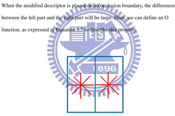
We modify the HOG descriptor by separating the original descriptor into two parts: left part and right part. Figure 3-15 (b) shows the modified HOG descriptor. When the modified descriptor is placed on an occlusion boundary, the differences between the left part and the right part will be large. Here, we can define an O function, as expressed in Equation 3.7 to describe this property.

Figure 3-15 Modified HOG descriptor

Now we apply the MHOG descriptor to the first term of the CRF model, MHOG is designed to handle occlusion effect. Here, we can write the data cost function as

𝜑𝑝 𝑑𝑝 [𝐻𝑂𝐺 𝐻𝑂𝐺 + 𝑑𝑝 ]*O (p) (3.6)

23

O p {1 , 𝑓 𝑒𝑓𝑒 𝑎𝑟𝑡 𝑑 𝑓𝑓𝑒𝑟𝑒𝑛𝑐𝑒 𝑟 ℎ𝑡 𝑎𝑟𝑡 𝑑 𝑓𝑓𝑒𝑟𝑒𝑛𝑐𝑒 < 𝛾

𝛤 , 𝑓 𝑒𝑓𝑒 𝑎𝑟𝑡 𝑑 𝑓𝑓𝑒𝑟𝑒𝑛𝑐𝑒 𝑟 ℎ𝑡 𝑎𝑟𝑡 𝑑 𝑓𝑓𝑒𝑟𝑒𝑛𝑐𝑒 ≥ 𝛾 (3.7)

In Equation 3.6, O(p) is an additional penalty function. Here, we check the feature vector at pixel p in the left image with the feature vector at the corresponding pixel p + 𝑑𝑝 in the right image. If the left-part feature distance of MHOG and the right-part feature distance of MHOG are inconsistent (e.g. one distance is small, another one is big), O(p) will multiply the data cost function in Equation 3.6) by 𝛤. In this case, the pixel p is more likely to be labeled as occluded. Figure 3-16 shows an example.

(a) Input images

(b) 𝛤 = 2 (c) 𝛤 3 Figure 3-16 Result comparison for different 𝛤 values

24

Figure 3-17 SIFT flow [21]

In comparison, as shown in Figure3-17, SIFT flow cannot detect occlusion regions. Hence, occluded regions are forced to match the most similar region.

3.2.4 Matching points by MHOG with spatially constraint

Now we will apply the MHOG descriptor to the CRF model. The adopted MHOG descriptor has a 24 x 24 window around pixels with two grids and eight orientations. Hence, the first term 𝜑_𝑝 (data cost) of the CRF formula is a distance of measure of the MHOG features between Pixel p on one image and Pixel p + 𝑑𝑝 on the other image. Since the MHOG provide the statistical information about gradient information, it can’t provide us enough spatial information. Hence, we use the second term to compensate for the lack of spatial information. In our experiments, we found that if a larger window is used, the MHOG feature component along the vertical orientation would be similar in different views similar. This is because we have placed cameras at the similar height without rolling. This character is used when we match feature pairs across images.

In summary, our CRF model has two terms, with the first term 𝜑_𝑝 𝑑𝑝 being discussed above. Our system will choose the disparity values that minimize the modified HOG distance over the whole image. The second term of CRF model is a

25

regularization term, which regulates the first term’s choice. This second term constrains adjacent pixels with similar intensity values to choose similar disparity values. This is because if a pixel and its neighbors have similar colors, then they probably come from the same surface of an object.

The regularization term of the CRF model is designed to be 𝛼 ∑ 𝐺 𝐼𝑝 _𝐼𝑞 _∗ 𝑝𝑞

𝑑𝑝_{, 𝑑}𝑞 _{, where p and q are neighbors and 𝐼}𝑝 _{is the intensity value of Pixel p. In}

this formula, if 𝐼𝑝 𝐼𝑞| < C (In our experimentation, C is chosen to be 30), 𝐺 𝐼𝑝 _𝐼𝑞 _{= 1. Moreover, 𝑑}𝑝_{, 𝑑}𝑞 _{is the L2 norm of the disparity difference}

between 𝑑𝑝 and 𝑑𝑞 . If two neighboring pixels have similar intensity values, they should choose similar disparity values.

26 3.2.5 Model formulation

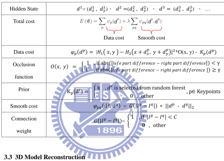
In Table 1 we summarize all related formulas of our CRF model.

Table 1 Model formulation

Hidden State 𝑑 = (𝑑_𝑥 , 𝑑_𝑦)、 𝑑 (𝑑_𝑥 , 𝑑_𝑦) 、 𝑑3 (𝑑_𝑥3 , 𝑑_𝑦3) 、 … Total cost

Data cost Smooth cost

Data cost 𝜑_𝑝 𝑑𝑝 |𝐻 ( 𝑥, 𝑦 ) 𝐻 (𝑥 + 𝑑_𝑥𝑝, 𝑦 + 𝑑_𝑦𝑝) *O(x, y) - 𝐾_𝑝 𝑑𝑝 Occlusion function 𝑂 𝑥, 𝑦 { _{Γ , if bs} 1 , if bs 𝑒𝑓𝑒 𝑎𝑟𝑡 𝑑 𝑓𝑓𝑒𝑟𝑒𝑛𝑐𝑒 𝑟 ℎ𝑡 𝑎𝑟𝑡 𝑑 𝑓𝑓𝑒𝑟𝑒𝑛𝑐𝑒 < γ 𝑒𝑓𝑒 𝑎𝑟𝑡 𝑑 𝑓𝑓𝑒𝑟𝑒𝑛𝑐𝑒 𝑟 ℎ𝑡 𝑎𝑟𝑡 𝑑 𝑓𝑓𝑒𝑟𝑒𝑛𝑐𝑒 ≥ γ Prior _K p dr { k , 𝑑 𝑟 _{is se ec ed fr m r nd m f res} 0 , her , p∈ Keyp in s Smooth cost 𝜑𝑝𝑞 𝑑𝑝, 𝑑𝑞 = 𝐺 𝐼𝑝 𝐼𝑞 ∗ 𝑑𝑝 - 𝑑𝑞 Connection weight 𝐺 𝐼𝑝 _𝐼𝑞 _{= {} 1 , if 𝐼𝑝 𝐼𝑞 < 𝐶 0 , her

3.3 3D Model Reconstruction

3.3.1 Camera calibration

After we have matched images and gotten pixel correspondence, we can use the correspondence to estimate the relative positions among the cameras. In other words, we can estimate each camera’s extrinsic parameter matrices 𝑅_𝑛 and 𝑇_𝑛, where 𝑅_𝑛 is a rotation matrix, 𝑇_𝑛 is a transformation matrix, and 𝑥′ = Rx + T. Figure 3-14 shows an example of the camera geometry.

27

3D to 2D projection matrix P, P = K*(R|T). After that, we can use the projection matrix P to find a 3D point cloud. Here, we apply the bundle adjustment algorithm used in [5] to build the 3D model.

Figure 3-19 Camera geometry

3.3.2 Bundle adjustment

The bundle adjustment in [22] can simultaneously refine the 3D coordinates to describe the scene geometry with the relative motion parameters. The bundle adjustment is based on the mathematical expression in Equation 3.8.

, , (3.8) where

𝑥

_𝑘 is the point correspondence between each image pair (in our system m = 3), 𝑃_𝑘 𝑋 is a 3D point 𝑋 projected to Image k via the projection matrix 𝑃_𝑘, and D(x, y) is the L2 norm distance between x and y. After minimizing the sum of projection error of all points, we can estimate the 3D point set that coarsely describes the view

28

geometry in front of cameras. The detail will be explained in the next section. After the estimation of the 3D point set, we use the spatial matting algorithm in [23, 24] to re-define the 3D point set. In Figure 3-20, we illustrate the finding of a 3D point cloud that minimizes the projection errors between the projected points on the 2D image and the original image points with inliers. To suppress outlier points, we use the RANdom SAmple Consensus method in [25] (RANSAC) to identify the inlier points.

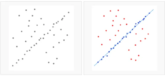
Figure 3-20 Estimation of 3D points by using bundle adjustment 3.3.3 Random sample consensus (RANSAC)

Random sample consensus is an iterative method to estimate the parameters of a mathematical model from a set of observed data which may contain outliers. We use RANSAC to estimate a camera model that fits the largest amount of inlier matches across images. Here, we use RANSAC to calculate the projection matrix for the first iteration of bundle adjustment.

29

Figure 3-21 (a) Data set with many outliers (b) Fitted line with RANSAC

3.3.4 3D point set refinement by matting refinement

In Section 3.3.2, we build a 3D point cloud by the bundle adjustment process. However, the outcomes are still not good enough. There are some false matches and several unmatched regions at occlusion pixels. We assume that our matches around keypoints are accurate and we build a confidence map CM(x, y). In Equation 3.9, if pixel (x, y) is near a keypoint, has an inlier matches (picked by RANSAC), and has no occlusion, then the confidence value at that pixel is equal to one; otherwise, the

confidence value is zero.

𝐶𝑀 𝑥, 𝑦 { 1 , if x, y ∈ Ne r keyp in s ∩ In iers ∩ N cc uded

30

Figure 3-22 (a) Locations of keypoints (b) Confidence map

After we estimate the depth information at these locations whose confidence value is one, by using the spectral matting method in [23, 26], we propagate these estimated depth information to these unknown regions by minimize the cost function in Equation 3.10, where L is a laplacian matrix, is a prior map (estimated depth map at confidence-one pixels). In Equation 3.12, is a 3×3 covariance matrix, is a 3×1 mean vector of the colors in a window _𝑘, and I₃ is the 3×3 identity matrix. The matting affinity in Equation 3.11 is defined by pixels’ color and its spatial relations (In Equation 3.12).

𝛼 𝛼+ (3.10) L = D – (3.11) , 𝑗 ∑ _𝑊 𝑘 1 + 𝐼 𝜇𝑘 ( 𝑘+ 𝜖 𝑊𝑘 𝐼3) − 𝑘 , ∈𝑊𝑘 Ij 𝜇𝑘 . (3.12)

In Equation 3.12, D is a diagonal matrix, whose elements are defined as D = ∑ 𝑊 , 𝑗 . W is a sum of matrix . is a prior map, at which we have

31

estimated the depth information at pixels with CM(x, y) =1. After we solve the

optimization problem in Equation 3.10, we can get all pixels’ depth values. A result of the aforementioned process is shown in Figure 3-23.

32

Figure 3-24 Overview of spectral matting

3.4 Summary

In our system, we combine local and global approaches to find the

correspondence of image pairs. First, we use randomized forest to obtain some rough correspondence of image keypoints. With the initial correspondence, we can

propagate these keypoints’ correspondence information to the entire image by solving a global optimization problem. Moreover, the CRF model can correct some errors by using spatial constraints. After we have gotten the disparity values of all pixels, we use the RANSAC method to find inliers whose distribution fits the camera geometry the most. After that, we use these inlier disparities to build a 3D point cloud and refine the 3D point cloud by spectral matting. Finally, we convert the point cloud to a mesh

33

of triangles and build the 3D model of the captured scene. The overall system flow is shown below.

34

Chapter 4 Experimental Results

In this chapter, we show some experimental results. In Section 4.1, we will demonstrate some matched correspondences, outcomes of random forest and the CRF model processing results, respectively. We can find that random forest only matches keypoints coarsely. In the next stage, the proposed CRF model will correct random forest’s result and also deal with those pixels lacking texture information.

4.1 Matched results

4.1.1 Matched results by using random forest

In Figure 4-1, an outdoor case, we observe that random forest can match some keypoints correctly. Figure 4-2 shows the correctly matched points. The match rate is about 30/100.

35

Figure 4-2 Some correct matches

In Figure 4-3 and Figure 4-4, we show the matching of some high-texture keypoints. (Red circles mean the incorrect correspondence.)

Figure 4-3 Matched result by random forest (part1)

36

In Figure 4-5, there are many repetitive patterns and regions with texture. As expected, the performance of this case is not good. However, after the CRF processing, we can still obtain many correctly matched pairs.

Figure 4-5 Matching result of random forest

37 4.1.2 Matched results after CRF correction

Figure 4-6 Result of CRF

Figure 4-7 Some matches of Figure 4-6

Figure 4-8 Some matches of Figure 4-6

In Figure 4-6, two images with difference exposure levels are matched by our system (random forest + CRF). We can find that CRF can correct some erroneous correspondence (some erroneous correspondences by random forest are shown in Figure 4-1) and can propagate a keypoint’s correspondence information to its

38

neighbors. (Here, we only demonstrate some keypoint correspondences.)

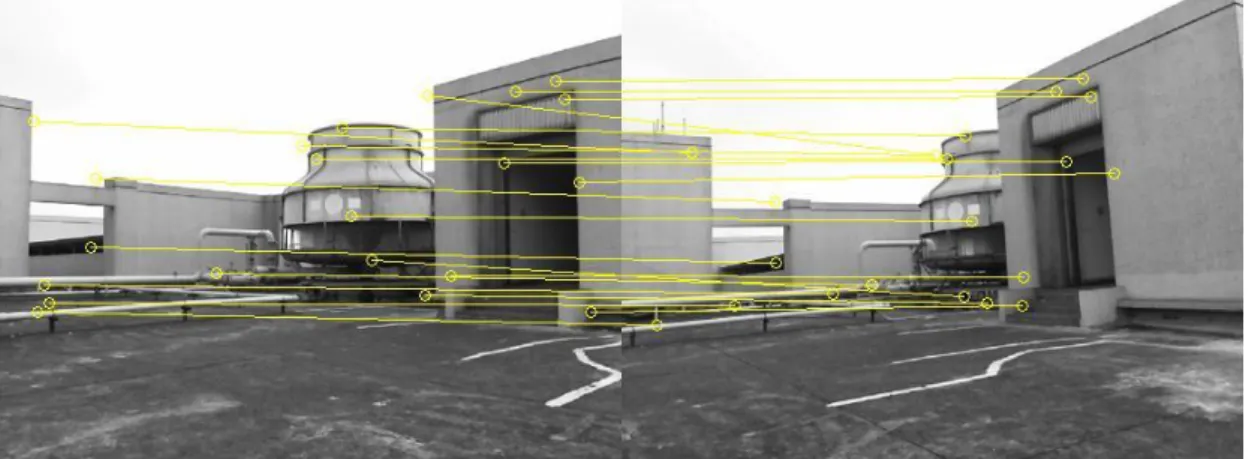
Next, we compare the SIFT matching result with our system, Figure 4-10 shows some correspondence results of our system. Note that the cameras are separated very widely and there are many low-texture areas and repetitive patterns in two images. The matching in this case is very difficult for the SIFT approach.

Figure 4-9 SIFT result (many mismatched points over the region with repetitive patterns)

(a) Our system (RF + CRF) can match repetitive patterns better than SIFT

(b) Our system (RF + CRF) can match repetitive patterns better than SIFT Figure 4-10 Some matched results of our system

39

In our system, we use a CRF model to match points with spatial constraints. Hence, we can identify similar patterns at difference locations. In brief, we can match keypoints better than the SIFT method.

40

4.2 3D Reconstruction

This section demonstrates some results of 3D reconstruction. Figure 4-12 shows our reconstruction result. It fails in these white lower texture regions, since these areas contain too little information for accurate matching.

(a) (b) (c)

(d) (e) (f)

41

Figure 4-13 Multi-view database “fountain” [7]

In Figure 4-13, we show the multi-view database “fountain” [7]. In [27], Hiep, V.H. and Keriven, R. reconstructed 3D models by using 11 stereo images. Their results are shown in Figure 4-16. Here, we only use 3 of the 11 images (the 3 images with red frame in Figure 4-13) to build the 3D model. As illustrated in Figure 4-14, we can see the object shape clearly in our reconstructed model.

(a)

(b)

42

Figure 4-15 First row: short-baseline input images. Second row: reconstructed 3D models

In Figure 4-15, we use short-baseline image pairs to build the 3D model. Here, we choose the images with green frames in Figure4-13. We can find that the details can be built more cleanly.

Figure 4-16 Hiep, V.H. and Keriven, R.’s results

43

Chapter 5 Conclusion

In this thesis, we proposed a wide-baseline stereo matching approach for 3D reconstruction. Our system can match images in difference illuminations with the change of viewpoint orientation ranging from about 40°to 40°. Based on random forest and conditional random field, the system can deal with large perspective distortions and occlusions. Besides, the proposed system can also deal with images with repetitive patterns. Matching similar patterns by using only gradient features usually cannot achieve robust and accurate matching. In our approach, we add the spatial information around each pixel to our matching strategy. With this arrangement, we can match similar patterns and distorted patterns well. In the last stage of our system, we use RANdom SAmple Consensus (RANSAC) and Bundle Adjustment (BA) to reconstruct 3D point cloud. Finally, we refine the 3D point cloud by using the spectral matting method and convert the point cloud to a mesh of triangles that

represent the 3D model of the captured scene.

44

Chapter 6 Reference

[1] N. Snavely, S. M. Seitz, and R. Szeliski, "Photo tourism: exploring photo collections in 3D." ACM Transactions on Graphics (TOG), pp. 835-846. [2] V. Lepetit, and P. Fua, “Keypoint recognition using randomized trees,” IEEE

Transactions on Pattern Analysis and Machine Intelligence, vol. 28, no. 9, pp. 1465-1479, 2006.

[3] V. Lepetit, P. Lagger, and P. Fua, "Randomized trees for real-time keypoint recognition." IEEE Conference on Computer Vision and Pattern Recognition, pp. 775-781 vol. 2., 2005.

[4] D. G. Lowe, “Distinctive image features from scale-invariant keypoints,” International Journal of Computer Vision, vol. 60, no. 2, pp. 91-110, 2004. [5] H. Bay, T. Tuytelaars, and L. Van Gool, “Surf: Speeded up robust features,” Computer Vision–European Conference on Computer Vision, pp. 404-417, 2006.

[6] K. Mikolajczyk, and C. Schmid, “A performance evaluation of local

descriptors,”IEEE Transactions on Pattern Analysis and Machine Intelligence, vol. 27, no. 10, pp. 1615-1630, 2005.

[7] C. Strecha. Multi-view evaluation-http://cvlab.epfl.ch/data, 2008.

[8] Y. Boykov, and V. Kolmogorov, “Computing geodesics and minimal surfaces via graph cuts,” IEEE International Conference on Computer Vision, pp. 26-33, 2003.

[9] C. Strecha, R. Fransens, and L. Van Gool, "Combined depth and outlier estimation in multi-view stereo." IEEE International Conference on Computer Vision, pp. 2394-2401, 2003

[10] D. Pritchard, and W. Heidrich, "Cloth motion capture." Computer Graphics Forum, pp. 263-271.

[11] Y. Amit, and D. Geman, “Shape Quantization and Recognition with

Randomized Trees,” Neural computation, vol. 9, no. 7, pp. 1545-1588, 1997. [12] L. Breiman, “Random Forests,” Machine learning, vol. 45, no. 1, pp. 5-32,

2001.

[13] H. Tin Kam, “Random decision forests,” in Proceedings of the Third

International Conference on Document Analysis and Recognition, 1995, pp. 278-282 vol.1.

[14] P. Geurts, D. Ernst, and L. Wehenkel, “Extremely randomized trees,” Machine learning, vol. 63, no. 1, pp. 3-42, 2006.

[15] J. Sivic, and A. Zisserman, "Video Google: a text retrieval approach to object matching in videos." IEEE International Conference on Computer Vision,pp.

45

1470-1477 vol.2, 2003.

[16] M. Calonder et al., “Brief: Binary robust independent elementary features,” Computer Vision–ECCV 2010, pp. 778-792, 2010.

[17] T. Kanade, and M. Okutomi, “A stereo matching algorithm with an adaptive window: Theory and experiment,” IEEE Transactions on Pattern Analysis and Machine Intelligence, vol. 16, no. 9, pp. 920-932, 1994.

[18] N. Salman, and M. Yvinec, "High resolution surface reconstruction from overlapping multiple-views." Proceedings of the 25th annual symposium on Computational geometry, pp. 104-105.

[19] N. Dalal, B. Triggs, and C. Schmid, “Human detection using oriented

histograms of flow and appearance,” Computer Vision–European Conference on Computer Vision, pp. 428-441, 2006.

[20] N. Dalal, and B. Triggs, "Histograms of oriented gradients for human

detection." IEEE Conference on Computer Vision and Pattern Recognition, pp. 886-893 vol. 1., 2005.

[21] C. Liu et al., “Sift flow: Dense correspondence across different scenes,” Computer Vision–European Conference on Computer Vision, pp. 28-42, 2008. [22] B. Triggs et al., “Bundle adjustment—a modern synthesis,” Vision algorithms:

theory and practice, pp. 153-177, 2000.

[23] A. Levin, A. Rav Acha, and D. Lischinski, “Spectral matting,” IEEE Transactions on Pattern Analysis and Machine Intelligence, vol. 30, no. 10, pp. 1699-1712, 2008.

[24] A. Levin, A. Rav-Acha, and D. Lischinski, "Spectral matting." IEEE Conference on Computer Vision and Pattern Recognition, pp.1-8, 2007.

[25] M. A. Fischler, and R. C. Bolles, “Random sample consensus: a paradigm for model fitting with applications to image analysis and automated cartography,” Communications of the ACM, vol. 24, no. 6, pp. 381-395, 1981.

[26] A. Levin, D. Lischinski, and Y. Weiss, “A closed-form solution to natural image matting,” IEEE Transactions on Pattern Analysis and Machine Intelligence, vol. 30, no. 2, pp. 228-242, 2008.

[27] V. H. Hiep et al., "Towards high-resolution large-scale multi-view stereo." IEEE Transactions on Pattern Analysis and Machine Intelligence, vol. 30, no. 10, pp. 1430-1437.