國
立
交
通
大
學
管理科學系
博
士
論
文
No. 023
預測公司破產事件之研究
On Bankruptcy Prediction
研 究 生:黃瑞卿
指導教授:李昭勝 教授
中 華 民 國 九 十 五 年 十 月
國
立
交
通
大
學
管理科學系
博
士
論
文
No. 023
預測公司破產事件之研究
On Bankruptcy Prediction
研 究 生:黃瑞卿
研究指導委員會:王耀德 教授
許和鈞 教授
謝國文 教授
指導教授:李昭勝 教授
中 華 民 國 九 十 五 年 十 月
預測公司破產事件之研究
On Bankruptcy Prediction
研 究 生:黃瑞卿 Student:Ruey-Ching Hwang
指導教授:李昭勝 Advisor:Jack C. Lee
國 立 交 通 大 學
管理科學系
博 士 論 文
A ThesisSubmitted to Department of Management Science College of Management
National Chiao Tung University in Partial Fulfillment of the Requirements
for the Degree of Doctor of Philosophy
in Management
October 2006
預測公司破產事件之研究
學生:黃瑞卿 指導教授:李昭勝博士
國立交通大學管理科學系博士班
摘 要
本文使用半母數羅吉特模型(semiparametric logit model)建立一個公司破產 事件的預測方法,並將之應用在追蹤性(prospective)或稱簡單隨機(simple random) 資料,以及個案控制(case-control)或稱選擇性(choice-based)資料。我們使用 區域概似方法(local likelihood approach)估計半母數羅吉特模型中未知參數, 且研究這些估計式的漸近偏差量與變異數(asymptotic bias and variance)。我們 證明當應用這個半母數羅吉特模型至前述兩種不同類型資料上,其所對應的破產預測 方法是相同的。因此我們的預測方法可以直接應用到這兩種重要類型的資料。實證研 究結果顯示,我們的預測方法較 Altman (1968)的區別分析模型(discriminant
analysis model)、Ohlson(1980)的線性羅吉特模型(linear logit model)、以及
Merton (1974)與 Bharath and Shumway (2004) 的 KMV-Merton 模型等所建立的預測
方法,能夠產生較小的樣本外誤差率(out-of-sample error rate)。
另外,本文使用離散型倖存模型(discrete-time survival model; Allison, 1982),預測公司發生財務危機的機率。我們以最大概似法(maximum likelihood method)估計該模型的參數值,導出參數估計式的漸近常態分配(asymptotic normal distribution),進而估計公司發生財務危機的機率。藉由此機率估計值,我們可建 立財務危機預警模型,並用以分析及預測台灣股票上市公司發生財務危機的機率。實 證研究結果顯示,本文所介紹的離散型倖存模型對公司財務危機的預測,比線性羅吉 特模型,有更好的樣本外預測能力。 關鍵詞:個案控制資料、離散型倖存模型、區別分析模型、KMV-Merton 模型、線性羅 吉特模型、追蹤性資料、半母數羅吉特模型、型 I 誤差率、型 II 誤差率。
On Bankruptcy Prediction
Student: Ruey-Ching Hwang Advisor: Dr. Jack C. Lee
Department of Management Science National Chiao Tung University
ABSTRACT
Bankruptcy prediction methods based on a semiparametric logit model are proposed for prospective (simple random) and case-control (choice-based) data. The unknown quantities in the model are estimated by the local likelihood approach, and the resulting estimators are analyzed through their asymptotic biases and variances. Our semiparametric bankruptcy prediction methods using these two types of data are shown to be essentially equivalent. Thus our proposed prediction model can be directly applied to data sampled from the two important designs. Empirical studies demonstrate that our prediction method is more powerful than alternatives based on the discriminant analysis model (Altman 1968), the linear logit model (Ohlson 1980), and the KMV-Merton model (Merton 1974; Bharath and Shumway 2004), in the sense of yielding smaller out-of-sample error rates.
The discrete-time survival model (Allison 1982) is applied to predict the probability of financial distress. The maximum likelihood method is employed to estimate the values of parameters in the model. The resulting estimates are analyzed by their asymptotic normal distributions, and are used to estimate the probability of financial distress for each firm under study. Using such estimated probability, a strategy is developed to identify failing firms, and is applied to study the probability of financial distress for firms listed in Taiwan
discrete-time survival model can yield more accurate out-of-sample forecasts than the alternative method based on the linear logit model in Ohlson (1980).
Keywords: case-control data, discrete-time survival model, discriminant analysis model, KMV-Merton model, linear logit model, prospective data, semiparametric logit model, type I error rate, type II error rate.
ACKNOWLEDGEMENTS
I wish to thank my advisor, Dr. Jack C. Lee, for his constant support, enthusiastic guidance, and helpful criticism in all parts of the research presented in this dissertation. I aslo wish to thank the other members of my committee, Dr. Chuang-Chang Chang, Dr. K.F. Cheng, Dr. Huimin Chung, Dr. Tsung-I Lin, Dr. Her-Jiun Sheu, Dr. G. Shieh, and Dr. Yau-De Wang for their valuable suggestions which substantially improve the research results.
I am grateful to the Department of Management Science and Graduate Institute of Finance for providing a good environment for study.
TABLE OF CONTENTS
ABSTRACT ( IN CHINESE) ………i
ABSTRACT ……….………ii
ACKNOWLEDGEMENTS ….………iv
TABLE OF CONTENTS ……….………v
LIST OF TABLES ………..………vii
LIST OF FIGURES ……….………..………viii
CHAPTER I: INTRODUCTION TO BANKRUPTCY PREDICTION METHODS …………1
1.1 Introduction ……….………1
1.2 Three Sampling Schemes ………4
1.3 The LLM ………6
1.4 The SLM ………9
1.5 The KMV ……….………14
1.6 The DAM ……….………17
1.7 The DSM ………..………18
1.8 Bankruptcy Prediction Devices ………22
1.9 Summary of Results ……….………25
CHAPTER II: SEMIPARAMETRIC BANKRUPTCY PREDICTION METHODS …………27
2.1 Introduction ………..…………27
2.2 Theoretical Results ………29
2.3 A Real Data Example ………33
2.4 A Simulation Study ………..…41
2.5 Discussion ………44
2.6 Sketches of the Proofs ………..………45
CHAPTER III: DYNAMIC PREDICTION METHODS FOR BANKRUPTCY AND FINANCIAL DISTRESS ………...………50
3.1 Introduction ………..………50
3.2 Theoretical Results ………51
3.3 A Real Data Example ………52
3.4 Discussion ………60
CHAPTER IV: CONCLUSIONS ……….………..62
LIST OF TABLES
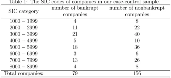
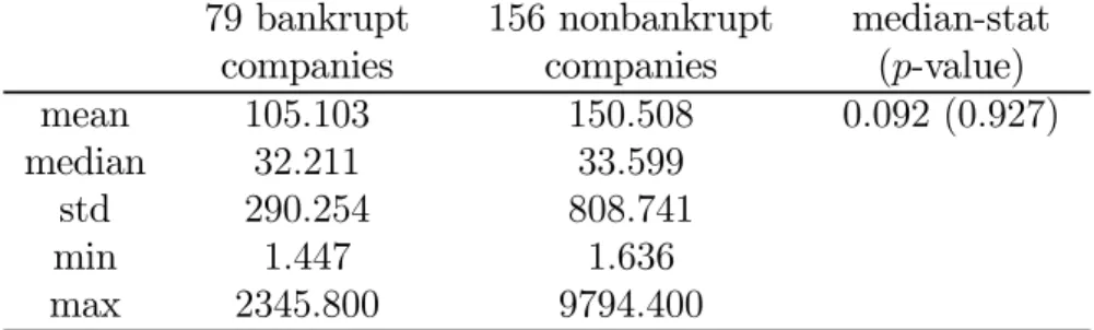
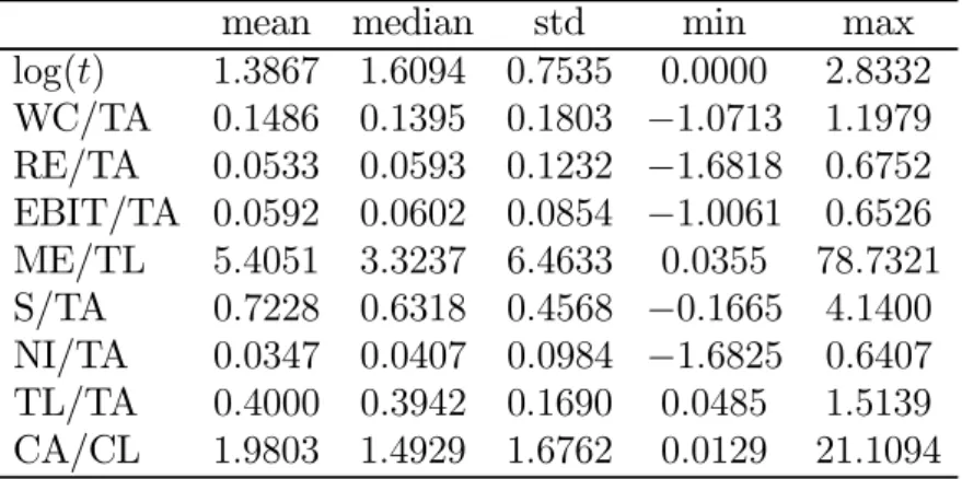
Table 1: The SIC codes of companies in our case-control sample .…..……….34 Table 2: Summary statistics of company asset sizes (in million US dollars) from our case-control sample ……….…….………..…...35 Table 3: Summary statistics of variables in our case-control sample ……….……..36 Table 4: Numerical results of the out-of-sample error rates obtained by applying KMV, DAM, LLM, and SLM to our case-control sample ………….……..………..41 Table 5: The information about industry and financial status of in-sample companies …54 Table 6: Summary statistics of variables in our discrete-time survival data ……….55 Table 7: The estimated values of parameters in each of the DSM and the LLM using our discrete-time survival data with Altman's predictors ….……….………56 Table 8: The estimated values of parameters in each of the DSM and the LLM using our discrete-time survival data with Zmijewski's predictors ………..57 Table 9: The selected optimal cutoff values ˆp obtained by applying each of the DSM * and the LLM to our discrete-time survival data with Altman's predictors, and those with Zmijewski's predictors ………..………..……….…..57 Table 10: The information about industry and financial status of out-of-sample companies ……...……….………..………58 Table 11: The out-of-sample error rates obtained by applying each of the DSM and the
LLM to our discrete-time survival data with Altman's predictors, and those with Zmijewski's predictors .………..…..………..60
LIST OF FIGURES
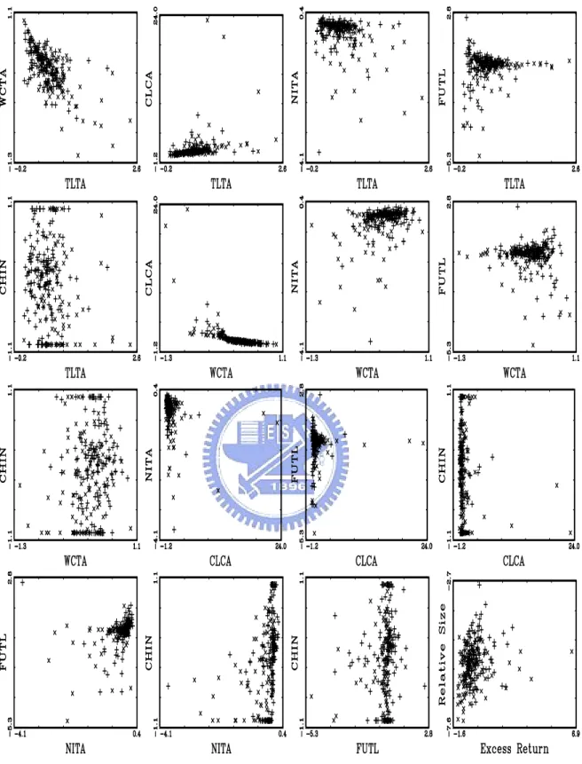
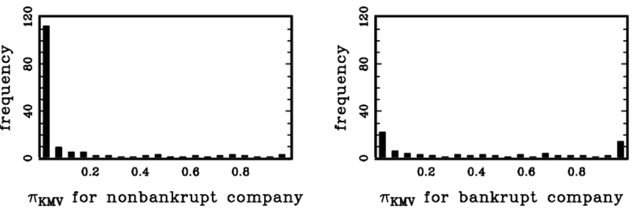
Figure 1: Pairwise scatter diagrams of our case-control sample ………...…38 Figure 2: The frequency histogram of the values of πKMV in our case-control sample .…39 Figure 3: The out-of-sample error rates obtained by applying KMV, DAM, LLM, and SLM to our case-control sample ………..………40 Figure 4: The out-of-sample error rates obtained by applying DAM, LLM, and SLM to our
simulated case-control data with the skewed Student t distribution for X ...42 Figure 5: The out-of-sample error rates obtained by applying DAM, LLM, and SLM to our
CHAPTER I
INTRODUCTION TO BANKRUPTCY PREDICTION METHODS
1.1 Introduction
Academics, practitioners and regulators have routinely used models to predict the bankruptcy of companies. For example, the discriminant analysis model (DAM) has been a popular technique for studying the financial health of a corporate; see Altman (1968). Other frequently referred models include the models by Ohlson (1980) and Zmijewski (1984). The former bankruptcy prediction method is based on a linear logit model (LLM). The latter, on the other hand, is based on a probit model. Grice and Dugan (2001) recently cautioned the routine application of these two probabilistic mod-els of bankruptcy. Their study showed that using the prediction modmod-els to time periods and industries other than those used to develop the models may result in significant decline in prediction accuracies.
Bankruptcy prediction methods using other models or concepts include, for exam-ple, the recursive partition model (Frydman, Altman, and Kao 1985), expert systems (Messier and Hansen 1988), chaos theory (Lindsay and Campbell 1996), neural networks (Koh and Tan 1999), survival analysis (Lane, Looney, and Wansley 1986; Shumway 2001; Chava and Jarrow 2004), rough set theory (McKee 2003), KMV-Merton model (KMV; Merton 1974; Bharath and Shumway 2004; Vassalou and Xing 2004), and sup-port vector machines (Härdle et al., 2006). Basically, these methods are more compli-cated in computation and interpretation than the above probabilistic models.
The bankruptcy prediction model in Ohlson (1980) postulates that the logit function of bankruptcy probability is a linear function of the predictors. Nine predictors were selected for developing his model because they appeared to be the ones most frequently mentioned in the literature. The main reason of using the LLM is due to its simplicity in computation and interpretation. There are many software packages having logistic regression capabilities, for example, BMDP, EGRET, GAUSS, GLIM, and SAS, etc.
Thus LLM can be easily updated or revised as long as there are new observations of the same predictors or new predictive variables available for analysis. For a detailed introduction of the LLM, see the monograph by Hosmer and Lemeshow (1989).
When appropriate, the LLM has definite advantages. For example, the correspond-ing inferential methods usually have nice efficiency properties. Also, the parameters generally have some physical meaning which makes them interpretable and of interest in their own right. If the assumed linear logit function is grossly in error, then the advantages of the LLM will not be realized. Thus, there are few benefits from using a poorly specified LLM. See the discussion and Figure 2 of Härdle, Moro, and Schäfer (2006). Their results show that the relation between the bankruptcy probability and predictors, such as net income change and company size, may not be monotonic. The LLM is most appropriate when theory, past experience, or other sources are available that provide detailed knowledge about the data under study. Sometimes, based on previous experience, there are reasons for modelling the logit function of bankruptcy probability as a particular parametric function of predictors, which may not be linear. However, a general drawback of such parametric modelling is that if one chooses a parametric family that is not of appropriate form, at least approximately, then there is still a danger of reaching erroneous inference.
The first focus of this dissertation is to consider a robust method, against misspec-ification of the parametric logit model relation, by introducing a semiparametric logit model (SLM; Zhao, Kristal, and White 1996) for predicting bankruptcy. This model is basically very similar to the LLM, except that some unspecified function replaces the linear function to model the relation between the predictors and the logit function of bankruptcy probability. Thus, clearly, the SLM is much more general and flexible in predicting the bankruptcy of a firm. Since the SLM is developed without assuming a parametric form for the logit function, there is some loss in the interpretability and efficiency of estimators obtained in this fashion. In contrast to physics or engineer-ing, it may not be often appropriate to give a specific functional relationship between
the probability of bankruptcy and the predictors in finance fields. Härdle, Moro, and Schäfer (2006) also propose a flexible but fully nonparametric approach for predicting bankruptcy. They use support vector machines to generate nonlinear score function of predictors, and then employ nonparametric technique to map scores into bankruptcy probabilities. Their work presents a new trend in bankruptcy analysis.
On the other hand, there is another potential pitfall of the LLM. It is static in nature, since it uses only one set of predictor values collected at a specific time point for each firm. The static model is generally not appropriate for predicting bankruptcy because it ignores both facts that the characteristics of firms change through time as well as bankruptcy does not often occur. For more discussions of the drawback to the static model, see Shumway (2001).
To avoid the drawback to the static model, Shumway (2001) applies the idea of time survival analysis (Cox and Oakes 1984) to develop the so-called discrete-time hazard model. The model has the advantage of using all available historical information to determine each firm’s bankruptcy risk at each point in time, hence it is a dynamic forecasting model. It is also called the discrete-time survival model (DSM) in Allison (1982). The values of parameters in Shumway’s dynamic prediction model are estimated by using the same approach as those in the multiperiod logit model (Pagano, Panetta, and Zingales 1998). However, theoretically, the multiperiod logit model assumes the predictor values collected for each firm at all time points are independent. Clearly, such predictor values are dependent, and the assumption does not hold in practice. Thus, asymptotic properties of the resulting estimates of parameters in Shumway’s dynamic prediction model can not be obtained from the multiperiod logit model.
The second focus of this dissertation is to employ directly the DSM to predict bank-ruptcy, and ignore the estimation procedure of the multiperiod logit model. The values of parameters in the DSM are estimated by the maximum likelihood method. The advantages of direct employment of the DSM include, for example, using all available
historical information to determine each firm’s bankruptcy risk at each point in time, assuming the predictor values of each firm are dependent. Hence, it is more general and flexible for the DSM to predict bankruptcy. The DSM has been successfully ap-plied in many fields including, for example, social science (Allison 1982), econometrics (Lancaster 1990), education (Singer and Willett 1993), and biostatistics (Klein and Moeschberger 1997).
The rest of this chapter is organized as follows. In Section 1.2, three important sampling schemes including the prospective (simple random), the case-control (choice-based), and the discrete-time survival data for bankruptcy prediction study are de-scribed. The data of the first two types are for static forecasting models, the LLM, the SLM, the KMV, and the DAM, and the data of the third type are for the dynamic forecasting model, the DSM. In Sections 1.3-1.7, five bankruptcy prediction models, the LLM, the SLM, the KMV, the DAM, and the DSM, are introduced respectively. In Sec-tion 1.8, bankruptcy predicSec-tion devices based on the five bankruptcy predicSec-tion models are presented. Finally, Section 1.9 contains a brief summary of the results obtained. 1.2 Three Sampling Schemes
In this section, the formulation of the data used in this dissertation for bankruptcy prediction study will be given. Three types of data including the prospective, the case-control, and the discrete-time survival data will be described in sequence.
Most bankruptcy prediction methods were developed on training samples. Usually, the training sample consists of the data of n companies collected for some time period by a simple random sampling scheme from the distribution of (X, Z). For the i-th company, i = 1, · · ·, n, we observe values (Yi, xi, zi), where Yi = 1 indicating that the i-th company is in the state of bankruptcy and 0, otherwise, and xi = (xi1, · · ·, xid)T and zi = (zi1, · · ·, ziq)T are values of the vectors of explanatory variables (X, Z) used to forecast failure. Here X and Z are the d-dimensional continuous and the q-dimensional discrete variables, respectively, and the upper index T stands for the transpose of a
matrix. Hence we have the prospective sample
(Yi, xi, zi), i = 1, · ··, n.
For example, in Ohlson (1980), there were 9 financial variables being used for developing his bankruptcy prediction model. Among these explanatory variables, 7 (= d) of them are continuous variables and 2 (= q) are binary variables.
On the other hand, the case-control data for bankruptcy prediction are composed of two simple random samples. One is selected from the population of bankrupt com-panies, and called the case sample. The other is selected from the population of non-bankrupt companies, and called the control sample. An important special case of the case-control study is the stratified (matched) case-control study. In the latter study, the number of cases (bankrupt companies) and controls (nonbankrupt companies) need not to be constant across strata, but most matched designs include one case and one to five controls per stratum and are thus referred to as 1-M matched designs. For a detailed introduction of the (matched) case-control data, see the monograph by Hosmer and Lemeshow (1989).
According to the case-control sampling, the case-control data are composed of a random sample of nonbankrupt companies of n0observations (controls), say (x1, z1), ···, (xn0, zn0), from the conditional distribution of (X, Z) given Y = 0, and an independent
random sample of bankrupt companies of n1 observations (cases), say (xn0+1, zn0+1),
· · ·, (xn, zn), where n = n0 + n1, from the conditional distribution of (X, Z) given Y = 1. Here Yi = 1 indicating that the i-th company is in the state of bankruptcy and 0, otherwise. Hence we have the case-control sample
(Yi, xi, zi), i = 1,· · ·, n, where Yi = 0 for i ≤ n0, and 1 for i > n0.
We now close this section by giving the formulation of the discrete-time survival data. The data are generated by three steps. Firstly, both the sampling period and
the sampling criteria are selected. For example, the sampling period may be taken as the one starting from January of the year 1981 to December of the year 1999, and the sampling criteria may be defined as those firms starting to be listed in Taiwan Stock Exchange during the sampling period. Secondly, n companies satisfying the sampling criteria are selected. Finally, all available historical information occurred at the discrete time points in the sampling period of n selected companies are collected. Hence we have the discrete-time survival data
(ti, Yi, xi,1, · ··, xi,ti, zi,1, · ··, zi,ti), for i = 1, · ··, n.
Here ti ∈ {1, 2, · · ·, m} denotes the duration time of the i-th company in the sampling period, and m is a positive integer standing for the length of the sampling period. Also, at the duration time ti, Yi = 0 indicates that the i-th company is nonbankrupt, and 1 the i-th company is bankrupt. Further, xi,j and zi,j are values of the d-dimensional continuous and q-dimensional discrete explanatory variables X and Z collected at the duration time j, respectively in each case, for each j = 1, · · ·, ti and for the i-th company.
1.3 The LLM
In this section, the formulation of the LLM using the prospective sample as well as that using the case-control sample for predicting bankruptcy will be introduced.
Given the prospective sample (Yi, xi, zi), i = 1, · · ·, n, the LLM is defined by assuming the bankruptcy probability for the company with the predictor values (X, Z) = (x, z)to be
p(Y = 1| X = x, Z = z) = exp(α + β x + θ z)
1 + exp(α + β x + θ z), (1)
or written in the form of the logit function of bankruptcy probability
logit{p(Y = 1 | X = x, Z = z)} = log ½
p(Y = 1| X = x, Z = z) ¾
Here α, β, and θ are 1 × 1, 1 × d, and 1 × q vectors of logistic parameters, respectively. For the company with predictor values (x0, z0), its predicted bankruptcy probability
ˆ
p(Y = 1| X = x0, Z = z0) =
exp(ˆα + ˆβ x0+ ˆθ z0) 1 + exp(ˆα + ˆβ x0+ ˆθ z0)
(2)
is the logistic distribution evaluated at the predicted score ˆα + ˆβ x0 + ˆθ z0. Here ˆα, ˆ
β, and ˆθ are maximum likelihood estimates for α, β, and θ, respectively, based on the prospective sample from the LLM (1).
The maximum likelihood approach for producing ˆα, ˆβ, and ˆθin (2) is now described. For this, set η = (α, β, θ)T. Using the prospective sample from the LLM (1), the log-likelihood function of η is LLM(η) = n X i=1 [Yi (α + β xi+ θ zi)− log{1 + exp(α + β xi+ θ zi)}] .
Then (ˆα, ˆβ, ˆθ)T may be taken as the solution of the normal equations
∂ LLM(η) ∂η = n X i=1 ∙ Yi− exp(α + β xi+ θ zi) 1 + exp(α + β xi+ θ zi) ¸ ⎡ ⎢ ⎢ ⎢ ⎢ ⎣ 1 xi zi ⎤ ⎥ ⎥ ⎥ ⎥ ⎦= 0. (3)
Due to the consistency of ˆα, ˆβ, and ˆθ (Hosmer and Lemeshow, 1989), the predicted bankruptcy probability exp(ˆα+ˆβ x0+ˆθ z0)
1+exp(ˆα+ˆβ x0+ˆθ z0) in (2) does converge to the true bankruptcy
probability exp(α+β x0+θ z0)
1+exp(α+β x0+θ z0) in (1) for the company with predictor values (x0, z0). By
this fact, it will be used in Section 1.8 to construct a bankruptcy prediction device for prospective data from the LLM (1).
On the other hand, using the case-control sample from the LLM (1) and treating the sample as if it was a prospective sample from the LLM (1), the maximum likelihood estimates for logistic parameters α, β, and θ are now given. Applying the case-control sample (Yi = 0, xi, zi) for i ≤ n0 and (Yi = 1, xi, zi) for i > n0 from the LLM (1) to the normal equations (3), Prentice and Pyke (1979) show that the resulting maximum
likelihood estimates ˆα, ˆβ, and ˆθof logistic parameters α, β, and θ, respectively, converge to their true values, except the intercept estimate ˆα, as both sample sizes of control and case data become large. This intercept estimate ˆα approaches the quantity α + c∗, where
c∗ = log{p(Y = 0) / p(Y = 1)} + log(n1 / n0).
Using the case-control sample, inferences about the constant c∗ are not possible since such data generally provide no information about the population frequency of bank-rupt companies. Unfortunately, due to the inconsistency of the intercept estimate ˆα and the fact that the unknown quantity c∗ is generally not equal to 0, the resulting predicted bankruptcy probability exp(ˆα+ˆβ x0+ˆθ z0)
1+exp(ˆα+ˆβ x0+ˆθ z0), obtained by plugging all these
es-timates of coefficients into (2), does not converge to the true bankruptcy probability exp(α+β x0+θ z0)
1+exp(α+β x0+θ z0) in (1), but approaches
exp(α+c∗+β x0+θ z0)
1+exp(α+c∗+β x0+θ z0), for the company with
pre-dictor values (x0, z0). This is the major difference between applying the LLM to the prospective sample and to the case-control sample. Although the predicted bankruptcy probability derived by the case-control sample from the LLM (1) does not estimate the true bankruptcy probability, we will discuss in Section 1.8 that it still can be used to develop a bankruptcy prediction device for case-control data from the LLM (1).
The main advantage of the LLM lies in its simplicity of computation and interpre-tation, but the model may not be efficient for the purpose of prediction. Sometimes, based on previous experience, there are reasons for modelling the logit function of bank-ruptcy probability as a particular parametric function of (X, Z), which may not be linear. However, a general drawback of such parametric modelling is that if one chooses a parametric family that is not of appropriate form, at least approximately, then there is a danger of reaching erroneous prediction. The limitation of LLM can be overcome by removing the restriction that the logit function of p(Y = 1 | X = x, Z = z) belongs to a parametric family. In Section 1.4, we shall use some unspecified function H(·) to replace the linear function to model the relation between the continuous predictors and the logit function of bankruptcy probability.
1.4 The SLM
In this section, the formulation of the SLM using the prospective sample and that using the case-control sample will be given. The SLM is defined similarly to the LLM (1) by replacing the linear relationship α + β x of the continuous predictor X in the logit function of the LLM with an unknown function H(x).
Given the prospective sample (Yi, xi, zi), i = 1, · · ·, n, the SLM is defined by assuming the bankruptcy probability for the company with the predictor values (X, Z) = (x, z) to be
p(Y = 1 | X = x, Z = z) = exp{H(x) + θ z}
1 + exp{H(x) + θ z}, (4)
or written in the form of the logit function of bankruptcy probability
logit{p(Y = 1 | X = x, Z = z)} = log ½ p(Y = 1| X = x, Z = z) 1− p(Y = 1 | X = x, Z = z) ¾ = H(x) + θz.
Here, we only assume H(x) to be a smooth function of the value x of the continuous predictor X, otherwise, it is not specified. Also, θ is a 1×q vectors of logistic parameters, as it does in the LLM (1). Clearly, this is a very flexible prediction model. For the company with predictor values (x0, z0), its predicted probability of bankruptcy is thus defined as ˆ p(Y = 1| X = x0, Z = z0) = exp{ ˆH(x0) + ˆθ z0} 1 + exp{ ˆH(x0) + ˆθ z0} , (5)
the logistic distribution evaluated at the predictive score ˆH(x0) + ˆθ z0. Here ˆH(x0) and ˆθ are estimates derived by applying the local likelihood method to the prospective sample from the SLM (4).
The local likelihood approach for producing ˆH(x0) and ˆθ in (5) is now introduced. This approach is composed of three steps. In the first step, an initial local likelihood estimate ˆH1(x0) of H(x0) is generated. There exists many methods for estimating
Tibshirani and Hastie (1987). This method is to first choose a positive scalar constant bθ, also called the bandwidth, and define a neighborhood of x0 as
N (x0; bθ) ={t = (t1,· · ·, td)T :|tj − x0j| ≤ bθ, for j = 1, · ··, d},
where x0 = (x01, · · ·, x0d)T. Then the idea of the local likelihood method is to apply both concepts of the weighted likelihood method using partial sample
S(x0; bθ) ={(Yi, xi, zi) : xi∈ N(x0; bθ), for i = 1, · ··, n},
and the first order Taylor approximation
H(xi)≈ H(x0) + H(1)(x0)T (xi− x0)≡ α + β (xi− x0),
for each xi ∈ N(x0; bθ). Here the larger the value of bθ, the larger the number of data points contained in S(x0; bθ). Also, the parameters α and β are 1×1 and 1×d vectors of parameters, respectively, as they are in the LLM. But, they now stand for the unknown quantities H(x0)and H(1)(x0)T, respectively, and H(1)(x0) is the d × 1 vector of partial derivatives of H(x0).
Specifically, to produce ˆH1(x0), a bankruptcy probability model developed by the above arguments
p(Y = 1| X = x, Z = z) = exp{α + β (x − x0) + θ z} 1 + exp{α + β (x − x0) + θ z}
(6)
is imposed to the prospective sample (Yi, xi, zi), i = 1, · · ·, n, from the SLM (4) with xi ∈ N(x0; bθ). Given the value of bθ and the resulting bankruptcy probability model (6) for the prospective sample from the SLM (4) with xi ∈ N(x0; bθ), the local
log-likelihood function of η = (α, β, θ)T is defined by SLM(η; x0) = n X i=1 Yi {α + β (xi− x0) + θ zi} Kbθ,i − n X i=1 log[1 + exp{α + β (xi− x0) + θ zi}] Kbθ,i, where Kbθ,i = Kbθ(xi− x0) = Qd
j=1K{(xi,j − x0,j)/bθ}. Here K(·) is called the kernel function, and is used to compute the weight assigned to the data. It is usually taken as a symmetric and unimodal probability density function over [−1, 1]. Hence it gives positive weight to the data inside the neighborhood sample S(x0; bθ) and weight 0 outside. The larger weights are given to data points with X values closer to x0 and
smaller weights to those with X values far from x0. However, the results from the
literature show that the choice of the density function K(·) is not very important in the local fitting. A popular choice of K(·) is the Epanechnikov kernel defined as
K(u) = (3/4) (1− u2) I(|u| ≤ 1);
see Wand and Jones (1995), due to its computational convenience and optimal per-formance (for example it minimizes mean square error among all nonnegative kernel functions).
Set the first element ˆα of the solution ˆη = (ˆα, ˆβ, ˆθ)of the normal equations
∂ SLM(η; x0) ∂η = n X i=1 ∙ Yi− exp(α + β (xi− x0) + θ zi) 1 + exp(α + β (xi− x0) + θ zi) ¸ ⎡ ⎢ ⎢ ⎢ ⎢ ⎣ 1 xi− x0 zi ⎤ ⎥ ⎥ ⎥ ⎥ ⎦Kbθ,i= 0 (7)
as the initial local likelihood estimate ˆH1(x0) of H(x0). By the same arguments for the consistency of the maximum likelihood estimate ˆα derived by (3) for the LLM (1),
ˆ
H1(x0) is a consistent estimate of H(x0). For this fact, see also Fan, Heckman, and Wand (1995).
Note that the concept of local inference is well established in regression analysis; see also Wand and Jones (1995). There are two major strategies considered in the local likelihood approach: using linear approximation (the first order Taylor approximation) for each H(xi) with xi ∈ N(x0; bθ), and using the partial (local) sample S(x0; bθ) to derive the maximum local likelihood estimates. This method is directly analogous to the LLM, except that here we have used the concept of local fitting.
In the second step, the estimate ˆθrequired in (5) is generated by applying the simple logistic regression analysis. To estimate the value of θ, we shall replace the unknown quantity H(xi)in the SLM (4) with its initial local likelihood estimate ˆH1(xi),for each i = 1, · · ·, n, fit the bankruptcy probability by the resulting model
p(Y = 1| X = xi, Z = zi) =
exp{α0+ ˆH1(xi) + θ zi} 1 + exp{α0+ ˆH1(xi) + θ zi}
, (8)
and use the prospective sample from the SLM (4) to maximize the corresponding pseudo profile log-likelihood function with respect to φ = (α0, θ)T. Here α0 is a normalizing constant which makes the bankruptcy probability function (8) be integrated to 1.
Specifically, using the bankruptcy probability model (8) and the prospective sample from the SLM (4), the pseudo profile log-likelihood function of φ = (α0, θ)T is
ˆSLM(φ) = n X i=1 h Yi {α0 + ˆH1(xi) + θ zi} − log[1 + exp{α0+ ˆH1(xi) + θ zi}] i .
Set (ˆα0, ˆθ)T as the solution of the normal equations
∂ ˆSLM(φ) ∂φ = n X i=1 " Yi− exp(α0+ ˆH1(xi) + θ zi) 1 + exp(α0+ ˆH1(xi) + θ zi) # ⎡ ⎢ ⎣1 zi ⎤ ⎥ ⎦ = 0. (9)
Hence the required estimate ˆθ of θ in (5) is obtained. By the results in Hosmer and Lemeshow (1989), the consistency of ˆθ for θ can be seen.
produced. To produce the value of ˆH(x0), follow the same arguments in the first step, replace the unknown quantity θ with ˆθ obtained in the second step, use the value of bandwidth bH, fit the bankruptcy probability by the resulting model
p(Y = 1| X = xi, Z = zi) =
exp{α∗+ β (x
i− x0) + ˆθ zi}
1 + exp{α∗+ β (xi− x0) + ˆθ zi} (10) for the prospective sample from the SLM (4) with xi ∈ N(x0; bH), and maximize the corresponding pseudo profile local log-likelihood function with respect to ξ = (α∗, β)T. Here α∗ and β stand for H(x0) + α1 and H(1)(x0)T, respectively, where α1 is a normal-izing constant which makes the bankruptcy probability function (10) be integrated to 1.
Specifically, using the value of bandwidth bH, the resulting bankruptcy probability model (10), and the prospective sample from the SLM (4), the pseudo profile local log-likelihood function of ξ = (α∗, β)T is ˆSLM(ξ; x0) = n X i=1 Yi {α∗+ β (xi− x0) + ˆθ zi} KbH,i − n X i=1 log[1 + exp{α∗+ β (xi− x0) + ˆθ zi}] KbH,i.
Set (ˆα∗, ˆβ)as the solution of the normal equations
∂ ˆSLM(ξ; x0) ∂ξ = n X i=1 " Yi− exp(α∗+ β(x i− x0) + ˆθzi) 1 + exp(α∗+ β(xi− x0) + ˆθzi) #⎡ ⎢ ⎣ 1 xi− x0 ⎤ ⎥ ⎦ KbH,i = 0. (11)
Combining the consistency of ˆθ and the consistency of the maximum likelihood esti-mates (ˆα∗, ˆβ) for (α∗, β), we see that the value of α1 converges to 0, as the sample size of prospective data become large. Hence ˆα∗ is a consistent estimate of H(x0), and the required estimate ˆH(x0) of H(x0) in (5) may be taken as ˆH(x0) = ˆα∗. For this fact, see also Fan, Heckman, and Wand (1995).
proba-bility exp{ ˆH(x0)+ˆθ z0}
1+exp{ ˆH(x0)+ˆθ z0} in (5) approaches the true bankruptcy probability
exp{H(x0)+θ z0}
1+exp{H(x0)+θ z0}
in (4) for the company with predictor values (x0, z0),as the sample size of prospective data become large. By this fact, it will be used in Section 1.8 to construct a bankruptcy prediction device for prospective data from the SLM (4).
On the other hand, using the case-control sample from the SLM (4) and treating the sample as if it was a prospective sample from the SLM (4), the local likelihood estimates for H(x0)and θ are now given. Applying the case-control sample (Yi = 0, xi, zi)for i ≤ n0 and (Yi = 1, xi, zi)for i > n0 from the SLM (4) to the normal equations (7), (9), and (11), the local likelihood estimates ˆH1(x0) and ˆH(x0)for H(x0)and ˆθ for θ can be produced. The consistency of both ˆH1(x0) and ˆH(x0) for H(x0) + c∗, and ˆθ for θ will be shown in Chapter II. Here
c∗ = log{p(Y = 0) / p(Y = 1)} + log(n1 / n0)
has been defined in Section 1.3.
Unfortunately, due to the consistency of ˆH(x0) for H(x0) + c∗ and the fact that the unknown quantity c∗ is generally not equal to 0, the resulting predicted bankruptcy probability exp{ ˆH(x0)+ˆθ z0}
1+exp{ ˆH(x0)+ˆθ z0}, obtained by plugging these ˆH(x0)and ˆθ into (5), does not
converge to the true bankruptcy probability exp{H(x0)+θ z0}
1+exp{H(x0)+θ z0} in (4), but approaches
exp{c∗+H(x0)+θ z0}
1+exp{c∗+H(x0)+θ z0}, for the company with predictor values (x0, z0). This is the major difference between applying the SLM to the prospective sample and to the case-control sample. Although the predicted bankruptcy probability (5) derived by the case-control sample from the SLM (4) does not estimate the true bankruptcy probability, we will discuss in Section 1.8 that it still can be used to develop a bankruptcy prediction device for case-control data from the SLM (4). The same conclusions have also been reached for the LLM in Section 1.3.
1.5 The KMV
will be introduced. The detailed computational procedure of the default probability can be referred to Bharath and Shumway (2004).
The KMV has two particularly important assumptions. The first one is that the total value of a firm is assumed to follow geometric Brownian motion:
dV
V = μ dt + σV dZ.
Here V is the total value of a firm, μ is the expected continuously compounded return on V , σV is the volatility of firm value, and Z is a standard Wiener process. The second assumption of the KMV is that the firm has issued just one discount bond maturing in T periods. Under these two assumptions, the equity of the firm is a call option on the underlying value of the firm with a strike price equal to the face value of the firm’s debt with a time-to-maturity of T . By the Black-Scholes call option pricing model, the equity value of a firm satisfies
E = V N (d1)− e−rT B N (d2). (12)
Here E is the market value of the firm’s equity, B is the face value of the firm’s debt, r is the risk-free interest rate, N (·) is the cumulative standard normal distribution function, and d1 = ln(V / B) + (r + σ2V / 2) T σV √ T , d2 = d1− σV √ T .
This formula (12) is called Black-Scholes-Merton option valuation equation. Hence, the value of equity is a function of the value of the firm and time, so it follows directly
from Ito’s lemma that σE = (V / E) (∂E / ∂V ) σV. By Black-Scholes-Merton option
valuation equation, it can be shown that ∂E/∂V = N (d1), so that under the assump-tions of the KMV , the volatilities of the firm value and its equity can be expressed by
σE = (V / E) N (d1) σV. (13) In order to implement the KMV, first it needs to compute the market value of the firm’s equity E by multiplying the firm’s shares outstanding by its current stock price. Second, it needs to estimate the volatility of equity from either historical stock returns data or from option implied volatility data. Third, it needs to choose a forecasting horizon T and a measure of the face value of the firm’s debt B. For example, it is common to assume T = 1, and take the book value of the firm’s total liabilities to be the face value of the firm’s debt. Fourth, it needs to collect values of the risk-free interest rate. After performing these steps, we have values for each of the variables in equations (12) and (13) except for the total value of the firm V and the volatility of firm value σV. Finally, it needs to simultaneously solve equations (12) and (13) numerically for values of V and σV. Once this numerical solution is obtained, by the assumptions of the KMV, the probability of default can be calculated as
πKMV = N (−DD), where DD = ln(V / B) + (μ− σ 2 V / 2) T σV √ T .
Simultaneously solving equations (12) and (13) is reasonably straightforward. How-ever, the probability of default is not obtained by simply solving these two equations numerically. Crosbie and Bohn (2001) explain that “In practice the market lever-age moves around far too much for [equation (13)] to provide reasonable results.” To resolve this problem, we compute the probability of default by implementing a com-plicated iterative procedure suggested by Bharath and Shumway (2004). The iterative procedure includes the following steps. First, we propose an initial value of σV = σE {E/(E + B)} and we use this value of σV and equation (12) to infer the market value of each firm’s assets at the end of every month for the previous year. Recall that E
is the market value of each firm’s equity and is calculated from CRSP database as the product of share price at the end of the month and the number of shares outstanding, B is the sum of the debt in current liabilities and one half of long term debt, σE is the annualized percent standard deviation of returns and is estimated from the prior year stock return data for each month, r is the risk free interest rate, and T = 1. Here r is taken as 1-Year Treasury Constant Maturity Rate obtained from the Board of Governors of the Federal Reserve system, and it is available from the website at http://research.stlouisfed.org/fred/data/irates/gs1. We then calculate the implied log return on assets each month and use that returns series to generate new estimates of σV and μ. We iterate on σV in this manner until it converges (so the absolute difference in adjacent σV is less than 10−3).
1.6 The DAM
In this section, the formulation of the DAM proposed by Altman (1968) for predict-ing bankruptcy will be introduced.
Given the sample (Yi, xi), i = 1, · · ·, n, the DAM for predicting bankruptcy for the company with the predictor value X = x is to compute the discriminant function value: DF V = (x1− x0)T Spooled−1 x, where x0 = ( n X i=1 xi I(Yi = 0) ) / ( n X i=1 I(Yi = 0) ) , x1 = ( n X i=1 xi I(Yi = 1) ) / ( n X i=1 I(Yi = 1) ) , Spooled = ( n X i=1 (xi− x1)(xi− x1)TI(Yi = 1) + n X i=1 (xi− x0)(xi− x0)TI(Yi = 0) ) /(n−2). The larger the value of DF V , the larger the possibility that the company having the predictor value X = x bankrupts. Given a cutoff value v, if DF V > v, then the
company is classified to be in the status of bankruptcy, otherwise it is classified as a
healthy company. The method for computing the optimal cutoff value v∗ for v will be
introduced in Section 1.8. For a detailed introduction of the DAM, see Johnson and Wichern (2002).
1.7 The DSM
In this section, the formulation of the DSM using the discrete-time survival data for predicting bankruptcy will be introduced.
The DSM is expressed by the likelihood function of the discrete-time survival data. Recall the discrete-time survival data given in Section 1.2:
(ti, Yi, xi,1, · ··, xi,ti, zi,1, · ··, zi,ti), for i = 1, · ··, n.
Here ti ∈ {1, 2, · · ·, m} denotes the duration time of the i-th company in the sampling period, and m is a positive integer standing for the length of the sampling period. Also, at the duration time ti, Yi = 0 indicates that the i-th company is nonbankrupt, and 1 the i-th company is bankrupt. Further, xi,j and zi,j are values of the d-dimensional continuous and q-dimensional discrete explanatory variables X and Z collected at the duration time j, respectively in each case, for each j = 1, · · ·, ti and for the i-th company.
To give the likelihood function of the discrete-time survival data, set f (t, x, z; ψ) as the conditional frequency function of T given (X, Z) = (x, z). Here T is a discrete random variable, T ∈ N = {1, 2, · · ·}, standing for the duration time of a given company, (x, z) are the values of explanatory variables (X, Z) observed at the duration time T = t, and ψ is a vector of parameters. Also, set the survivor function of the given company as
S(t, x, z; ψ) = 1−X
j<t
time t for the given company. Further, set the hazard function of the given company as
h(t, x, z; ψ) = f (t, x, z; ψ)
S(t, x, z; ψ) = p(T = t| T ≥ t, x, z; ψ). (15)
The hazard function (15) gives the probability of bankruptcy happened instantly at the duration time t for the given company which is nonbankrupt before the duration time t.
We now give the likelihood function of the discrete-time survival data (ti, Yi, xi,1, · · ·, xi,ti, zi,1, · · ·, zi,ti), for i = 1, · · ·, n. Using the conditional frequency function
f (t, x, z; ψ),it can be written as L(ψ) = n Y i=1 p(Ti = ti | xi,ti, zi,ti; ψ) Yi p(T i > ti | xi,ti, zi,ti; ψ) 1−Yi = n Y i=1 f (ti, xi,ti, zi,ti; ψ) Yi p(T i > ti | xi,ti, zi,ti; ψ) 1−Yi.
Using elementary properties of conditional probabilities, each of the two probabilities f (ti, xi,ti, zi,ti; ψ) and p(Ti > ti | xi,ti, zi,ti; ψ) in the likelihood function L(ψ) can be
expressed as a function of the hazard function (15). For this, using (15) and replacing S(t, x, z; ψ) with f (t, x, z; ψ) + p(T > t | x, z; ψ), we have
f (t, x, z; ψ) = h(t, x, z; ψ) {f(t, x, z; ψ) + p(T > t | x, z; ψ)}.
On both sides of the equation, first subtracting f (t, x, z; ψ) h(t, x, z; ψ), and then dividing by h(t, x, z; ψ), we have
{1 − h(t, x, z; ψ)} S(t, x, z; ψ) = p(T > t | x, z; ψ).
to p(T > j | x, z; ψ) for each j = 1, · · ·, t, we have t
Y j=1
{1 − h(j, x, z; ψ)} = p(T > t | x, z; ψ). (16)
On the other hand, using (15) and (16), we have
f (t, x, z; ψ) = h(t, x, z; ψ) t−1 Y j=1
{1 − h(j, x, z; ψ)}. (17)
Substituting (16) and (17) into the above likelihood function L(ψ) for the discrete-time survival data, it can be expressed as
L(ψ) = n Y i=1 ½ h(ti, xi,ti, zi,ti; ψ) 1− h(ti, xi,ti, zi,ti; ψ) ¾Yi Yti j=1 {1 − h(j, xi,j, zi,j; ψ)}. (18)
Note that the hazard function (15) can be of any functional form whose values are all in the interval (0, 1). In this dissertation, for simplicity of presentation, it is taken as a logistic function
h(t, x, z; ψ) = exp{α0+ α1 g(t) + β x + θ z} 1 + exp{α0+ α1 g(t) + β x + θ z}
,
where ψ = (α0, α1, β, θ)T. Here α0, α1, β,and θ are 1×1, 1×1, 1×d, and 1×q vectors of logistic parameters, respectively. In this dissertation, the function g(t) is taken as g(t) = log(t). Substituting the logistic hazard function h(t, x, z; ψ) = exp{α0+α1g(t)+β x+θ z}
1+exp{α0+α1 g(t)+β x+θ z}
and the natural logarithm function g(t) = log(t) into the likelihood function L(ψ) in (18), the DSM for the discrete-time survival data is expressed as
L(ψ) = n Y i=1
[exp{α0+ α1 log(ti) + β xi,ti + θ zi,ti}
Yi
×
ti
Y j=1
[1 + exp{α0+ α1 log(j) + β xi,j+ θ zi,j}]−1. (19) If the function g(t) of the duration time t is taken as the natural logarithm function,
then the resulting DSM (19) is an accelerated failure-time model; see Lancaster (1990). Such logistic hazard function with g(t) = log(t) is also considered by Shumway (2001). We now give the maximum likelihood estimates ˆα0, ˆα1, ˆβ, and ˆθ of α0, α1, β, and θ, respectively. Using the DSM (19) and the discrete-time survival data, the log-likelihood function of ψ = (α0, α1, β, θ)T is
DSM(ψ) =
n X
i=1
Yi {α0+ α1 log(ti) + β xi,ti + θ zi,ti} −
n X i=1 ti X j=1
log[1 + exp{α0 + α1 log(j) + β xi,j + θ zi,j}].
Then ˆψ = (ˆα0, ˆα1, ˆβ, ˆθ)T may be taken as the solution of the normal equations
0 = ∂ DSM(ψ) ∂ψ = n X i=1 Yi ⎡ ⎢ ⎢ ⎢ ⎢ ⎢ ⎢ ⎢ ⎣ 1 log(ti) xi,ti zi,ti ⎤ ⎥ ⎥ ⎥ ⎥ ⎥ ⎥ ⎥ ⎦ − n X i=1 ti X j=1
exp{α0+ α1 log(j) + β xi,j+ θ zi,j} 1 + exp{α0+ α1 log(j) + β xi,j+ θ zi,j}
⎡ ⎢ ⎢ ⎢ ⎢ ⎢ ⎢ ⎢ ⎣ 1 log(j) xi,j zi,j ⎤ ⎥ ⎥ ⎥ ⎥ ⎥ ⎥ ⎥ ⎦ .
Using the maximum likelihood estimates ˆα0, ˆα1, ˆβ, and ˆθ, for the company with predictor values (X, Z) = (x0, z0) at the duration time t, its predicted probability of instant bankruptcy
h(t, x0, z0; ˆψ) =
exp{ˆα0+ ˆα1 log(t) + ˆβ x0+ ˆθ z0} 1 + exp{ˆα0+ ˆα1 log(t) + ˆβ x0+ ˆθ z0}
(20)
is the logistic hazard function evaluated at the predicted score ˆα0+ ˆα1 log(t) + ˆβ x0+ ˆθ z0. Due to the consistency of maximum likelihood estimates ˆα0, ˆα1, ˆβ, and ˆθ (Section 3.3 of Cox and Oakes 1984), the predicted probability of instant bankruptcy exp{ˆα0+ ˆα1 log(t) + ˆβ x0+ ˆθ z0} / [1 + exp{ˆα0+ ˆα1 log(t) + ˆβ x0+ ˆθ z0}] in (20) converges to the true probability of instant bankruptcy exp{α0+α1 log(t)+β x0+θ z0}
1+exp{α0+α1 log(t)+β x0+θ z0}, the logistic hazard
predictor values (x0, z0)at the duration time t. By this fact, it will be used in Section 1.8 to construct a bankruptcy prediction device for the DSM with the discrete-time survival data.
1.8 Bankruptcy Prediction Devices
In this section, we shall develop bankruptcy prediction methods for the five models, LLM, SLM, KMV, DAM, and DSM, in sequence.
Using the prospective training sample from the LLM (1), we determine a p∗ ∈ (0,
1)value to make bankruptcy prediction for the company with predictor values (x0, z0). By the consistency of its predicted bankruptcy probability ˆp(Y = 1| X = x0, Z = z0) derived from (2), if it satisfies
ˆ
p(Y = 1| X = x0, Z = z0) > p∗,
then the company is classified to be in the status of bankruptcy, otherwise it is classified as a healthy company. To decide a proper cut-off point p∗, usually one would use the training sample to evaluate the performance of the classification scheme. In doing so, there are two types of “in-sample” error rate occurred in this evaluation based on the training sample:
type I error rate αin(p) =
Pn i=1 Yi I{ˆp(Y = 1| X = xi, Z = zi)≤ p} Pn i=1 Yi , and
type II error rate βin(p) =
Pn
i=1 (1− Yi) I{ˆp(Y = 1| X = xi, Z = zi) > p}
Pn
i=1 (1− Yi)
.
Here I(·) stands for the indicator function. Using the training sample and the cut-off point p, αin(p)is the rate of misclassifying bankrupt company to healthy company, and
βin(p) is the rate of misclassifying healthy company to bankrupt company. To keep
that
τin(p∗) = αin(p∗) + βin(p∗) = min
p∈[0,1], αin(p)≤u{α
in(p) + βin(p)}.
That is to control the in-sample type I error rate αin(p)to be at most u, so that the sum of the two in-sample error rates τin(p) = αin(p) + βin(p) is minimal. This is essential if the type I error would cause much more severe losses to the investors. On the other hand, if classifying healthy firms as being bankrupt would cause more severe losses to the investors, we might control the in-sample type II error rate βin(p) to be at most u. In practice, the value of u ∈ [0, 1] is determined by the investor. If u = 1, then there is no restriction on the magnitude of in-sample type I and II error rates (Altman, 1968; Ohlson, 1980; Begley, Ming, and Watts, 1996). Since the value of p∗ depends on that of u, it is also denoted by p∗(u).
On the other hand, using the case-control training sample from the LLM (1) and treating the sample as if it was a prospective sample from the LLM (1), by the results in Section 1.3, the corresponding predicted bankruptcy probability exp(ˆα+ˆβ x0+ˆθ z0)
1+exp(ˆα+ˆβ x0+ˆθ z0)
obtained from (2) does not converge to the true bankruptcy probability exp(α+β x0+θ z0)
1+exp(α+β x0+θ z0)
in (1), but approaches exp(α+c∗+β x0+θ z0)
1+exp(α+c∗+β x0+θ z0). Here c∗ = log{p(Y = 0)/p(Y = 1)} +
log(n1/n0). This drawback is caused by the fact that the resulting maximum likelihood estimates ˆβ and ˆθ of logistic parameters β and θ in the LLM (1) converge to their true values, respectively, but ˆα approaches the quantity α + c∗, as both sample sizes of control and case data become large. This is the major difference between applying the LLM to case-control data and to prospective data.
Fortunately, we still can use the predicted bankruptcy probability exp(ˆα+ˆβ x0+ˆθ z0)
1+exp(ˆα+ˆβ x0+ˆθ z0)
obtained by the case-control sample from the LLM (1) to develop a bankruptcy predic-tion device by applying the following simple equivalent inequalities:
exp{α + β x + θ z}
if and only if
exp{α + c∗+ β x + θ z} 1 + exp{α + c∗+ β x + θ z} >
p exp(c∗)
(1− p) + p exp(c∗) ≡ pc∗.
This result is to say that using the probability 1+exp(α+β x+θ z)exp(α+β x+θ z) to define classification device with cut-off point p is equivalent to using the probability 1+exp(α+cexp(α+c∗+β x+θ z)∗+β x+θ z) to
define classification device with cut-off point pc∗. Hence we may pretend the predicted
bankruptcy probability exp(ˆα+ˆβ x0+ˆθ z0)
1+exp(ˆα+ˆβ x0+ˆθ z0) obtained by the case-control sample from the
LLM (1) to be the estimate of the true bankruptcy probability and use it to determine the corresponding proper cut-off point p∗(u). Then the bankruptcy prediction device for the case-control sample from the LLM (1) can be obtained.
Note that above bankruptcy prediction methods built for the LLM (1) using the two types of data are essentially equivalent. Based on the same arguments, similar bankruptcy prediction devices can be developed directly for the SLM (4) using the two types of data by replacing respectively (2) and ˆα + ˆβ x0 with (5) and ˆH(x0). Hence the bankruptcy prediction methods constructed for the SLM (4) using the two types of data are also essentially equivalent.
Note also that the above method for computing the optimal cutoff value for the LLM
(1) can be similarly applied for both the KMV and the DAM by replacing ˆp(Y = 1|
X = x0, Z = z0)with πKMV and DF V to derive their optimal cutoff values π∗KM V and v∗, respectively in each case. Given the optimal cutoff value π∗
KM V, if πKM V > π∗KM V, then the company with the probability of default πKM V is classified to be in the status of bankruptcy, otherwise it is classified as a healthy company. Similarly, given the optimal cutoff value v∗, if DF V > v∗, then the company with the discriminant function value DF V is classified to be in the status of bankruptcy, otherwise it is classified as a healthy company.
We now give the bankruptcy prediction method for the DSM. Using the discrete-time survival data and following the same arguments of the bankruptcy method based
prediction for the company with predictor values (x0, z0) at the duration time t. By the consistency of its predicted probability of instant bankruptcy h(t, x0, z0; ˆψ), if it satisfies
h(t, x0, z0; ˆψ) > p∗,
then, at the duration time t, the company is classified to be in the status of bankruptcy, otherwise it is classified as a healthy company. To decide a proper cut-off point p∗, we use the data (ti, Yi, xi,ti, zi,ti), for i = 1, · · ·, n, to evaluate the performance of the
classification scheme. In doing so, there are two types of “in-sample” error rate occurred in this evaluation based on the data (ti, Yi, xi,ti, zi,ti), for i = 1, · · ·, n:
type I error rate αin(p) =
Pn
i=1 Yi I{h(ti, xi,ti, zi,ti; ˆψ)≤ p}
Pn
i=1 Yi
,
and
type II error rate βin(p) =
Pn
i=1 (1− Yi) I{h(ti, xi,ti, zi,ti; ˆψ) > p}
Pn
i=1 (1− Yi)
.
Here I(·) stands for the indicator function. To keep these two error rates to be as small as possible, we determine a proper cut-off point p∗ = p∗(u) for the bankruptcy prediction method based on the DSM such that
τin{p∗(u)} = αin{p∗(u)} + βin{p∗(u)} = min
p∈[0,1], αin(p)≤u{α
in(p) + βin(p)},
for each u ∈ [0, 1]. 1.9 Summary of Results
In Chapter II, the SLM (4) with case-control sampling is applied to estimate bank-ruptcy probabilities for firms collected from Compustat North America (COMPUSTAT) and Center for Research in Security Prices (CRSP) databases. The unknown quanti-ties in the model are estimated by the local likelihood approach, and the resulting estimators are analyzed through their asymptotic biases and variances. Both a real
data example and a simulation study demonstrate that, given case-control data, our semiparametric prediction method based on the SLM (4) is more powerful than the prediction method based on the LLM (1), the KMV, and the DAM, in the sense of yielding smaller out-of-sample error rate.
In Chapter III, the DSM (19) with discrete-time survival data is applied to estimate the probabilities of financial distress for firms listed in Taiwan Stock Exchange. Since there are only few bankrupt firms in Taiwan, it is difficult to predict bankruptcy well. In this case, to provide more failure firms to proceed our research, we replaced our target on bankruptcy prediction with financial distress prediction. According to the definition of financial distress given by Taiwan Stock Exchange, financial distress companies are those whose stocks were delisted, stopped trading, or traded by cash. The maximum likelihood method is employed to estimate the values of parameters in the DSM, and the resulting estimators are analyzed by their asymptotic normal distributions. Empirical studies demonstrate that the financial distress prediction method based on the dynamic DSM (19) using discrete-time survival data can yield more accurate forecasts than the alternative method based on the static LLM (1), in the sense of yielding smaller out-of-sample error rate.
In Chapter IV, some concluding remarks and future research topics for bankruptcy prediction methods based on each of the static SLM (4) and the dynamic DSM (19) are presented.
CHAPTER II
SEMIPARAMETRIC BANKRUPTCY PREDICTION METHODS
2.1 Introduction
As introduced in Sections 1.3 and 1.4, the SLM (4) is a robust method against misspecification of the parametric logit model relation for predicting bankruptcy. This model is basically very similar to the LLM (1), except that some unspecified function H(x)replaces the linear function α + β x to model the relation between the continuous predictors and the logit function of bankruptcy probability. Thus, clearly, the SLM is much more general and flexible in predicting the bankruptcy of a firm.
In this section, we shall first study the asymptotic properties of estimators ˆH1(x), ˆ
θ, and ˆH(x) given in Section 1.4 for the SLM with case-control data. Then the finite sample performance of the bankruptcy prediction method based on the SLM with case-control data is studied through a real data example and a simulation study. For these, the composition of the case-control sample and the formulations of these estimators are recalled.
According to the case-control sampling, we draw a random sample of nonbankrupt companies of n0 observations (controls), say (x1, z1), ···, (xn0, zn0), from the conditional
distribution of predictors (X, Z) given Y = 0, and an independent random sample of bankrupt companies of n1 observations (cases), say (xn0+1, zn0+1), · · ·, (xn, zn), where
n = n0 + n1, from the conditional distribution of predictors (X, Z) given Y = 1. Here Yi = 1 indicating that the i-th company is in the state of bankruptcy and 0, otherwise. Hence we have the case-control sample (Yi, xi, zi), i = 1, ···, n, where Yi = 0for i ≤ n0, and 1 for i > n0. Set f (x, z) as the frequency function of predictors (X, Z), and f0(x, z) = f (x, z | Y = 0) and f1(x, z) = f (x, z | Y = 1) as the conditional frequency functions of (X, Z) given Y = 0 and 1, respectively. Then from Bayes theorem and the SLM (4), these two conditional frequency functions can be related by
where
H∗(x) = H(x) + log{p(Y = 0) / p(Y = 1)}.
Given the case-control sample and the bandwidth parameters bθ and bH, by the de-velopment of the logistic regression in the case-control setting given in both Section 1.4 of this dissertation and Section 6.3 of Hosmer and Lemeshow (1989), the log-likelihood functions for producing ˆH1(x), ˆθ, and ˆH(x)in the SLM (4) with kernel function K can be expressed respectively as 1(α, β, θ; x) = (−1) n X i=1 log[1 + exp{α + β (xi− x) + θ zi)}] Kbθ(xi− x) + n X i=n0+1 {α + β (xi− x) + θ zi} Kbθ(xi− x), (22) 2(α0, θ) = (−1) n X i=1 log[1 + exp{α0+ ˆH1(xi) + θ zi)}] + n X i=n0+1 {α0+ ˆH1(xi) + θ zi}, (23) 3(α∗, β; x) = (−1) n X i=1 log[1 + exp{α∗+ β (xi− x) + ˆθ zi)}] KbH(xi− x) + n X i=n0+1 {α∗+ β (xi− x) + ˆθ zi} KbH(xi− x). (24)
Note that the parameter β in (22) and (24) represents the unknown quantity H(1)(x)T, as it did in SLM(η; x0) and ˆSLM(ξ; x0) in Section 1.4 with x0 replaced by x. But α and α∗ in (22) and (24) stands for H(x) + c∗, not as they did in
SLM(η; x0) and ˆSLM(ξ; x0) in Section 1.4 for H(x) with x0 replaced by x, respectively in each case.
The maximum likelihood estimates of α and α∗ produced from (22) and (24) would be
estimates for H(x)+c∗, not for H(x). This fact causes the major difference between the applications of the logit model to the case-control sample and the prospective sample
This chapter is organized as follows. Section 2.2 presents asymptotic properties of estimators ˆH1(x), ˆθ, and ˆH(x) introduced in Section 1.4 for the SLM (4) with case-control data. To illustrate the bankruptcy prediction method based on the SLM with case-control data, a real data set is analyzed in Section 2.3. Simulation results which give additional insight of the bankruptcy prediction method are contained in Section 2.4. Section 2.5 gives concluding remarks and future research topics. Finally, sketches of the proofs are given in Section 2.6.
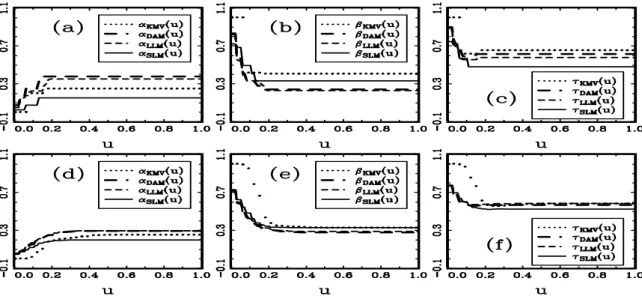
2.2 Theoretical Results
In this section, we shall study the asymptotic properties of ˆH1(x), ˆθ, and ˆH(x). For this, we need the following conditions:
(C1) Kernel function K(u) is a symmetric and Lipschitz continuous probability density function supported on [−1, 1], and is bounded above zero on [−1/2, 1/2].
(C2) n0/n→ ζ ∈ (0, 1), as n → ∞.
(C3) Bandwidth parameters bθ, bH ∈ [δ n−1+δ, δ−1n−δ], for some δ satisfying 0 < δ < 1/2. They also satisfy n bd+2θ >> 1 >> bθ and n bdH >> 1 >> bH >> bθ. The notation an>> bn means that bn/an→ 0, as n → ∞.
(C4) The d-variate function H(x) is defined on [0, 1]d, and each of its second order partial derivatives is Lipschitz continuous on [0, 1]d.
(C5) Under control and case populations, their respective marginal densities f0(x)and f1(x) of X are Lipschitz continuous and bounded above zero on [0, 1]d. Also, their corresponding conditional probabilities f0(z | x) and f1(z | x) of Z given X = x can not be zero or one for each given x, and are Lipschitz continuous with respect to x.
Conditions (C1)-(C4) are regular for the usual nonparametric regression analysis.
The support [0, 1]d in (C4) and (C5) of the d-dimensional variable X is given for
simplicity of presentation and for studying the asymptotic behavior of ˆH1(x)and ˆH(x) on the boundary region of the support of f0(x)and f1(x). It can be replaced with any bounded region Ω ⊂ Rd, and the asymptotic properties for the resulting ˆH
ˆ
H(x) remain unchanged. The first part of condition (C5) guarantees that the design
points X, under control and case populations, have no holes on [0, 1]d. The second part of (C5) makes sure that the Hessian matrix for each of 1(α, β, θ; x) and 3(α, β; x) is invertible.
In order to give concise expressions for the asymptotic properties of ˆH1(x), ˆθ, and ˆ
H(x), we need more notations. Let
x = (x1, · ··, xd)T, t = (t1, · ··, td)T, Hij(x) = ∂2/(∂xi ∂xj) H(x), mi = max{−1, (xi− 1)/b}, ki = min{1, xi/b}, K#(t) = d Y j=1 K(tj), λ0 = Z k1 m1 · · · Z kd md K#(t) dt, τ0 = Z k1 m1 · · · Z kd md K#(t)2 dt, λi,k = Z ki mi uk K(u) du, cij = Z k1 m1 · · · Z kd md ti tj K∗(t) dt,
Qbe the collection of all values of the discrete q-dimensional variable Z, and I1 be the (1 + q)× (1 + q) identity matrix with the first column vector of the identity matrix deleted, for i, j = 1, · · ·, d and k ≥ 0. Here K∗(t) is the d-variate Lejeune-Sarda kernel function of order two (Lejeune and Sarda 1992). In particular, given the point x ∈ [0, 1]d, the kernel function K, and the bandwidth b, K∗(t)can be expressed as
K∗(t) = ( d Y i=1 λ−1i,0 K(ti) ) ( 1− d X i=1
(ti λi,0− λi,1) λi,1 (λi,0 λi,2− λ2i,1)−1 )
,
and its corresponding values cij become
cij= ⎧ ⎪ ⎨ ⎪ ⎩
(λ2i,2− λi,1 λi,3) (λi,0 λi,2− λ2i,1)−1, for i = j, (−1) λi,1 λ−1i,0 λj,1 λ−1j,0, for i 6= j. Define
r(x, z) = f0(x, z) exp{H(x) + c
∗+ θ z} ζ + (1− ζ) exp{H(x) + c∗+ θ z}},
D0(x) = X z∈Q r(x, z), D1(x) = X z∈Q z r(x, z), D2(x) = X z∈Q z zT r(x, z), Dj = Z 1 0 · · · Z 1 0 Dj(x) dx, for j = 0, 1, 2, D = ⎛ ⎜ ⎝ D0, D T 1 D1, D2 ⎞ ⎟ ⎠ .
Also, define quantities related to the asymptotic biases and variances of ˆH1(x), ˆθ, and ˆ H(x)in the following: cH(x; b) = (1/2) d X i=1 d X j=1 cij Hij(x), vH,1(x; b) = D0(x)−1 Z k1 m1 · · · Z kd md K∗(t)2 dt, vH,2(x; b) = λ−20 τ0 D0(x)−1 D1T(x) © D0(x) D2(x)− D1(x) DT1(x) ª−1 D1(x), cθ(b) = (−1) ∙Z 1 0 · · · Z 1 0 {D0(x), DT1(x)} cH(x; b) dx ¸ D−1 I1, vθ = D−12 D1 (D0− D1T D2−1 D1)−1 D1T D2−1 + D−12 .
If x is in the interior region [b, 1 − b]d of [0, 1]d, then it can be seen that the values of cH(x; b) and vH,1(x; b)become cH(x; b) = (1/2) ½Z 1 −1 u2 K(u) du ¾ (Xd i=1 Hii(x) ) , vH,1(x; b) = D0(x)−1 ½Z 1 −1 K(u)2 du ¾d .
The following Theorem 2.1 states the asymptotic bias and variance for ˆH1(x), and those for ˆθ and ˆH(x). The proofs will be given in Section 2.6.
Theorem 2.1. Under the SLM and the case-control sample, suppose that conditions (C1)-(C5) are satisfied. For each x ∈ [0, 1]d
and as n → ∞,
Var{ ˆH1(x)} = n−1b−dθ ζ−1(1− ζ)−1 {vH,1(x; bθ) + vH,2(x; bθ)} + O(n−1b−d+1θ ), (26) Bias(ˆθ) = E(ˆθ)− θ = b2θ cθ(bθ) + O(b3θ+ n−1b−dθ ), (27)
Var(ˆθ) = n−1 ζ−1(1− ζ)−1 vθ+ O(n−1bθ), (28)
Bias{ ˆH(x)} = E{ ˆH(x)} − H(x) − c∗ = bH2 cH(x; bH) + O(b3H+ b 2
θ+ n−1b−dH ), (29)
Var{ ˆH(x)} = n−1b−dH ζ−1(1− ζ)−1 vH,1(x; bH) + O(n−1b−d+1H ). (30)
Remark 2.1. {The optimal kernel function K and the magnitudes of the optimal
bandwidth parameters b∗
θ and b∗H for constructing ˆθ and ˆH(x)} By Theorem 8 of Fan, Gasser, Gijbels, Brockmann, and Engel (1993) and our Theorem 2.1, the optimal K satisfying the conditions in (C1) for constructing ˆH(x) is the Epanechnikov kernel K(u) = (3/4) (1− u2) I(
|u| ≤ 1), for each x ∈ [0, 1]d, in the sense of having smaller asymptotic mean square error. On the other hand, by (29) and (30), the optimal choice of bH, in terms of having smallest mean square error of ˆH(x), is b∗H = c∗H n−1/(d+4), where c∗
H is a constant depending on the unknown factors H(·), θ, and f0(x, z). Similarly, by (25)-(28) and (C3), the optimal value b∗
θ of bθ, in terms of having smallest mean square error of ˆθ, satisfies the condition n−1/(d+4) >> b∗θ >> n−1/(d+2). Hence we conclude that the value of b∗
H is of larger order than that of b∗θ, and that the mean square error of ˆ
H(x)using the optimal bandwidth parameter b∗
H is of smaller order in magnitude than that of ˆH(x)using b∗
θ.
Remark 2.2. {Selection of values of bθ and bH for practically constructing ˆθ and ˆH(x), respectively} The practical implementation of SLM requires the specification of each
value of bθ and bH. It determines how many data points should be included in the
SLM. The optimal values b∗θ and b∗H of bθ and bH, respectively, can be determined by minimizing the mean square errors of the resulting ˆθ and ˆH(x). Theoretical results
in Remark 2.1 show that b∗
H is of larger order in magnitude than b∗θ. Although such theoretical results give some indication on how to select bandwidth parameters bθ and bH, they are not available in practice, since they depend on the unknown H(·), θ, and
density function of the predictors. Thus, in real applications, we would suggest to consider the in-sample type I and II error rates defined in Section 1.8 as functions of the cut-off point p and values of bθ and bH, denoted as αin(p, bθ, bH)and βin(p, bθ, bH), respectively. The cut-off point and the bandwidth parameters are then simultaneously determined so that the sum of the two in-sample error rates τin(p, bθ, bH) = αin(p, bθ, bH) + βin(p, bθ, bH)is minimal, subject to the constrains: p ∈ [0, 1], αin(p, bθ, bH)≤ u, and bH ≥ bθ, for each given value of u ∈ [0, 1]. Let ˆp(u), ˆbθ(u), and ˆbH(u) denote such selected values for p∗(u), b∗
θ, and b∗H, respectively.
2.3 A Real Data Example
In this section, a real case-control data set is analyzed using our method SLM and prediction rules DAM, LLM and KMV. McKee (2003) pointed out that company asset size and industry are significant factors affecting bankruptcy status. Thus an ideal approach is to stratify companies according to industry and asset size and determine prediction model for each stratum. Unfortunately, we did not have enough data from COMPUSTAT and CRSP databases for doing so. Thus, to illustrate our method, we simply used two controls to match with one case so that they had the same standard industrial classification (SIC) code and similar company asset size from the same year. By doing this, it is clear that the company asset size has no more power in discriminating the bankruptcy status of the company and thus will not be included in the analysis of our example.
We now introduce the case-control data set. The data set contains 79 companies that were delisted and declared bankruptcy (cases) during the period 1994 to 2002 by COMPUSTAT as meeting the Chapter 11 Bankruptcy or Chapter 7 Liquidation. Af-ter identifying these companies filing for bankruptcy, both COMPUSTAT and CRSP databases were searched to locate the latest annual financial data prior to the delist-ing date. Thus the annual financial data for the identified bankrupt companies were from the period 1993 to 2001. Among the 79 selected bankrupt companies, each was matched with two nonbankrupt companies, except 2 companies only matched with one