具複合型屬性之特徵群聚與選取

全文

(1)國立高雄大學資訊工程學系(研究所) 碩士論文. 具複合型屬性之特徵群聚與選取 Feature Clustering and Selection with Composite Attributes. 研究生：宋偉屏指導教授：洪宗貝. 撰博士. 中華民國九十九年七月.

(2) 誌謝雖然只有短短的二年，但在這碩士的求學生涯中，我學到了很多能讓我一生都授用的。洪宗貝老師，雖然我大三時就跟你作事了，但你當時擁有的豐富專業學識和良好的指導讓我在讀碩士班時的第一時間就決定由你來繼續當我的指導老師，雖然實驗室的事情很多，但相對的卻也過的很充實。也由於老師無悔的指導，這二年我學到了很多東西，也變的比以前更外向了，在此獻上萬分的謝意。我要感謝我的口試委員們，高大洪宗貝老師、林文揚老師，台南李健興老師，中山林葭華老師，由於你們在口試期間給予的建議與指教，使我的論文更趨完整，也由於你們專業的知識，讓我了解到自己所學到的還只是冰山一角，仍然還有一大部分是我還要去努力學習的。我還要感謝實驗室的同仁們，Jerry、欣怡、國誠、俊豪、明泰和韋体等學長姐們，你們幫助了我很多，我有很多不會的事都是由你們細心的指導我才會的，雖然一開始認識你們時覺得有時你們很嚴肅，但後來才知道並沒有這回事。廷一、國棟，我們一起努力打拼完成研究，有好多事都是跟你們互相幫忙一起完成的。宗慶、世濱、峰世等其他學弟們，跟你們相處真的很快樂，整個碩二的時間有大部分都是跟你們一起度過。謝謝實驗室的大家，由於你們的陪伴，這個求學生涯才不會枯燥乏味。我還要感謝我的家人，由於你們的支持，我才能無後顧之憂的全力攻讀我的碩士學位。我還要感謝小熊偉偉，雖然只有短短的一年，但也由於你的陪伴，才能讓我在人生中留下精彩的一刻。最後，這二年來真的很感謝大家的陪伴和幫助，我才能順利的完成研究所的學業，謝謝你們。宋偉屏謹致民國 99 年 7 月.

(3) Feature Clustering and Selection with Composite Attributes. Advisor: Dr.(Professor) TZUNG PEI HONG Department of Computer Science and Information Engineering National University of Kaohsiung Student: WEI PING SONG Department of Computer Science and Information Engineering National University of Kaohsiung. Abstract Feature selection is an important pre-processing step in data mining and machine learning. An properly selected feature subset can not only reduce computational time to derive rules but also decrease classification cost. It is usually executed when the amount of attributes in a given training data is very large. In the past, some researches about feature extraction by feature clustering were proposed, but all of them considered clustering single attributes. In this thesis, we propose two GA-based clustering methods for composite-attribute clustering and feature selection. In the first method, a new chromosome representation is presented, which is divided into two parts, the composition part and the cluster part. The composition part is used to represent which attributes can be combined into a composite attribute, and the cluster I.

(4) part is used to denote which cluster an attribute is located in. The fitness of each individual is evaluated using the average accuracy of the composite or single attribute substitutions in clusters, the cluster balance and the total penalty for the composite attributes. The second method further extends the first one to improve the time performance. A new fitness function based on the accuracy, composition penalty, cluster balance and the attribute similarity is proposed. It can reduce the time of scanning training sets. Besides, we design an adjustment process to make the composite attributes consistent with their cluster numbers. At last, experiments are done and the experimental results show the proposed approaches can obtain a good performance and get a good trade-off between accuracy and time complexity. The proposed approaches can thus provide flexible alternatives for feature selection and can also easily handle the problem of missing values in classification.. Keywords: Feature Selection; Feature Clustering; Genetic Algorithm; Composite Attribute; Chromosome Representation.. II.

(5) 具複合型屬性之特徵群聚與選取指導教授：洪宗貝博士（教授）國立高雄大學資訊工程所學生：宋偉屏國立高雄大學資訊工程所. 中文摘要特徵選取的技術在資料探勘與機器學習上扮演著相當重要的角色，當訓練用的資料集合具備大量的特徵個數時，其所需要的計算時間通常是相當可觀的，而特徵選取的技術可以來處理此一問題。一組優良的特徵集合在分類問題上不只可以擁有著高準確率並且可以減少探勘所需的時間。在過去，已經有一些藉由特徵群聚來進行特徵擷取的研究了，但都只考慮到單一屬性。因此，在這篇論文內，我們提出了二個基於基因演算法來進行複合式屬性的分群以及特徵選取。在第一個方法中，提出了一個新的染色體編碼，此編碼分成二個部分，屬性組合的部分和分群的部分。屬性組合的部分代表著哪些特徵會組合成複合式屬性，而分群的部分代表著這些特徵所歸屬的群聚。我們利用不同群聚內的特徵組合出來的集合之分類準確度與各群間特徵數量的平衡度和複合式屬性所持有的懲罰值來評估一個染色體的好壞。第二個方法則是延伸第一個方法並提出一個新的適應度函數來改進時間的效能。此新的適應度函數採用了不同群聚內的特徵組合出來的集合 III.

(6) 之分類準確度、屬性之間的相似程度、各群間特徵數量的平衡度和複合式屬性所持有的懲罰值來進行染色體的評估，其可大量減低掃描資料庫所需的時間。除此之外，我們提出了一個針對複合式屬性的分群部分的錯誤的調整程序。最後的實驗部分討論我們所提的方法所求得的分群結果，證實可以得到良好的效能，並且可在準確率與計算時間之間達成折衷。我們所提出的特徵分群方法比以往的特徵選取技術有更大的彈性，而且也可以輕易的處理在分類時特徵值遺失的問題。. 關鍵字: 特徵選取，特徵群聚，基因演算法，複合式屬性，染色體編碼。. IV.

(7) Content ABSTRACT............................................................................................... I 中文摘要..................................................................................................III CHAPTER 1 INTRODUCTION.............................................................1 1.1 BACKGROUND AND MOTIVATION ..........................................................................1 1.2 CONTRIBUTIONS ....................................................................................................4 1.3 THESIS ORGANIZATION .........................................................................................5. CHAPTER 2 REVIEW OF RELATED WORKS .................................6 2.1 FEATURE SELECTION .............................................................................................6 2.2 REDUCT ................................................................................................................8 2.3 OBJECT CLUSTERING...........................................................................................10 2.4 GENETIC ALGORITHMS........................................................................................11 2.5 GENETIC ALGORITHMS APPLIED TO CLUSTERING ...............................................12 2.6 ATTRIBUTE CLUSTERING AND FEATURE SELECTION WITH ATTRIBUTE SIMILARITY ............................................................................................................................14 2.7 ATTRIBUTE CLUSTERING AND FEATURE SELECTION BASED ON GENETIC ALGORITHMS ............................................................................................................15. CHAPTER 3 ............................................................................................17 3.1 ACCURACY ..........................................................................................................19 3.2 COMPOSITION PENALTY ......................................................................................21. CHAPTER 4 GA-BASED CLUSTERING FOR COMPOSITE ATTRIBUTES .........................................................................................23 4.1 CHROMOSOME REPRESENTATION ........................................................................23 V.

(8) 4.2 INITIAL POPULATION ...........................................................................................24 4.3 FITNESS AND SELECTION .....................................................................................25 4.4 GENETIC OPERATORS ..........................................................................................32 4.5 CLUSTER ADJUSTMENT .......................................................................................39 4.6 THE PROPOSED ALGORITHM ...............................................................................42 4.7 AN EXAMPLE ......................................................................................................44. CHAPTER 5 GA-BASED CLUSTERING FOR COMPOSITE AND SINGLE ATTRIBUTES WITH SIMILARITY...................................52 5.1 FITNESS FUNCTION .............................................................................................52 5.2 THE PROPOSED ALGORITHM ...............................................................................62 5.3 AN EXAMPLE ......................................................................................................65. CHAPTER 6 EXPERIMENTAL RESULTS........................................74 6.1 EXPERIMENTAL RESULTS OF THE FIRST APPROACH .............................................75 6.2 EXPERIMENTAL RESULTS OF THE SECOND APPROACH .........................................82. CHAPTER 7 CONCLUSIONS AND FUTURE WORKS ..................92 REFERENCES........................................................................................94. VI.

(9) List of Figures Figure 2.1: The conventional framework of feature selection .......................................7 Figure 2.2: The entire GA process ...............................................................................12 Figure 3.1: An example for attribute composition and clustering ...............................18 Figure 3.2: The plot of the penalty function with N = 8 and γ = 0.5 .........................22 Figure 4.1: A more-balanced clustering result .............................................................28 Figure 4.2: A less-balanced clustering result ...............................................................28 Figure 4.3: The results after the first kind of crossover...............................................34 Figure 4.4: The results after the second kind of crossover ..........................................35 Figure 4.5: The results after the third kind of crossover..............................................36 Figure 4.6: The results after the mutation....................................................................38 Figure 4.7: An example for the adjustment process.....................................................41 Figure 4.8: An example in the adjustment process with a tie ......................................41 Figure 4.9: The six offspring for the three kinds of crossover by C1 and C2 ...............48 Figure 4.10: The six offspring chromosomes after the cluster adjustment..................49 Figure 4.11: The offspring of O1 after the mutation operation ....................................49 Figure 4.12: The six offspring chromosomes after the mutation operation.................49 Figure 4.13: The offspring O1 ' after the cluster adjustment. .......................................50 Figure 4.14: The six offspring chromosomes after the cluster adjustment..................50 Figure 5.1: An example for finding the center of each cluster.....................................59 Figure 5.2: The six offspring for the three kinds of crossover operators.....................71 Figure 5.3: The six offspring chromosomes after the cluster adjustment....................71 Figure 5.4: The offspring of O1 after the mutation operation ......................................72 Figure 5.5: The six offspring chromosomes after the mutation operation...................72 Figure 5.6: The offspring O1 ' after the cluster adjustment ..........................................73 VII.

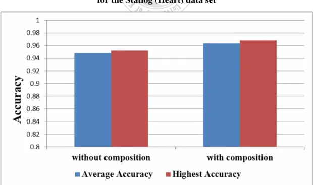
(10) Figure 5.7: The six offspring chromosomes after the cluster adjustment....................73 Figure 6.1: The average and the highest accuracy for the Statlog (Heart) data set .....75 Figure 6.2: The average and the maximum cluster balance for the Statlog (Heart) data set ..............................................................................................................76 Figure 6.3: The average total penalty for the Statlog (Heart) data set .........................77 Figure 6.4: The average and the highest accuracy without composite attributes for the Statlog (Heart) data set..............................................................................78 Figure 6.5: The comparison of the feature clustering approaches with and without composite attributes for K = 3 for the Statlog (Heart) data set .................78 Figure 6.6: The average and the highest accuracy for the Wine data set.....................79 Figure 6.7: The average and the maximum cluster balance for the Wine data set.......80 Figure 6.8: The average total penalty for the Wine data set ........................................80 Figure 6.9: The average and the highest accuracy without composite attributes for the Wine data set .............................................................................................81 Figure 6.10: The comparison of the feature clustering approach with and without composite attributes for K = 3 for the Wine data set...............................81 Figure 6.11: The average and the highest accuracy of second method for the Statlog (Heart) data set........................................................................................82 Figure 6.12: The average and the maximum cluster balance of second method for the Statlog (Heart) data set ...........................................................................83 Figure 6.13: The average similarity measures of second method for the Statlog (Heart) data set ....................................................................................................84 Figure 6.14: The average total penalty of second method for the Statlog (Heart) data set ...........................................................................................................84 Figure 6.15: The average and the highest accuracy without composite attributes of second method for the Statlog (Heart) data set.......................................85 VIII.

(11) Figure 6.16: The comparison of the second feature clustering approaches with and without composite attributes for K = 3 for the Statlog (Heart) data set..86 Figure 6.17: The average and the highest accuracy of second method for the Wine data set ....................................................................................................87 Figure 6.18: The average and the maximum cluster balance of second method for the Wine data set...........................................................................................87 Figure 6.19: The average similarity measures of second method for the Wine data set ................................................................................................................88 Figure 6.20: The average total penalty of 10 runs of second method for the Wine data set............................................................................................................88 Figure 6.21: The average and the highest accuracy without composite attributes of second method for the Wine data set ......................................................89 Figure 6.22: The comparison of the second feature clustering approaches with and without composite attributes for K = 3 for the Wine data set .................89 Figure 6. 23: The comparison of the execution time between the two approaches for the Statlog (Heart) data set .....................................................................90 Figure 6. 24: The comparison of the execution time between the two approaches for the Wine data set ....................................................................................90. IX.

(12) List of Tables Table 2.1: A simple information system ......................................................................10 Table 3.1: A training example dataset U with 7 attributes and 10 objects ...................20 Table 4.1: An example for chromosome representation ..............................................24 Table 4.2: Two chromosomes for crossover ................................................................33 Table 4.3: The mask sequence in the example.............................................................33 Table 4.4: The results after the adjustment for the first kind of crossover operation ..35 Table 4.5: The results after the adjustment for the second kind of crossover operation ....................................................................................................................36 Table 4.6: The results after the adjustment for the third kind of crossover operation .37 Table 4.7: The results after the adjustment ..................................................................39 Table 4.8: Ten objects in the example..........................................................................44 Table 4.9: The four initial chromosomes .....................................................................45 Table 4.10: The fitness values of all the chromosomes in the example.......................47 Table 5.1: An example dataset U with 7 attributes and 10 objects ..............................55 Table 5.2: The similarity table in the example.............................................................57 Table 5.3: Ten objects in the example..........................................................................65 Table 5.4: The four initial chromosomes .....................................................................66 Table 5.5: The similarity table of the example.............................................................67 Table 5.6: The fitness values of all the chromosomes in the example.........................70 Table 6.1: The characteristics of the Statlog (Heart) data set ......................................74 Table 6.2: The characteristics of the Wine data set......................................................74. X.

(13) CHAPTER 1 Introduction 1.1 Background and Motivation Feature selection is an important pre-processing step in data mining and machine learning [11]. A good subset of features can not only reduce execution time of deriving rules [4], but also improve accuracy of classification. Feature selection is thus very critical to data classification and data retrieval. It has been widely used in many research fields such as pattern recognition, statistics, data mining, and among others. Feature selection is always executed especially when the amount of attributes in a given training set is large. Some feature selection techniques have been proposed to handle this problem [2][33]. They select some relevant attributes to deal with the data efficiently and effectively. Finding an optimal feature subset has, however, been shown to be an NP-hard problem [5]. Some researches thus focused on balancing the computation complexity and the optimality of the results [7]. No matter which method was used, a suitable evaluation method was needed to measure the goodness of a feature subset. For example, one of the famous approaches for feature selection is 1.

(14) based on the rough-set theory [26][27], which was proposed by Pawlak in 1982. In the theory, the reduced set of attributes (features) is called a “reduct” and the minimum reduct was desired to classify a dataset with the expectation of being processed faster than on an original entire set of attributes [19][34][35]. In the approach, the minimal reduct could be thought of as the desired evaluation criterion. Besides, some other methods for finding out approximate reducts were proposed as well. Wróblewski used the genetic algorithm to find out approximate minimal reducts [32]. Sun and Xiong also tried to find approximate minimal reducts but in an incomplete information systems [29]. Al-Radaideh et al. used the discernibility matrix and a weighting strategy to find minimal reducts in a greedy way [1]. Gao et al. proposed a feature ranking strategy (similar to attribute weighting) with a sampling process included [8]. Besides, Hong and Liou proposed a feature selection approach based on the concept of feature clustering [15]. Their approach could not only find out an approximate reduct for classification but also cluster the attributes with high similarity into the same cluster. Its advantage was that attributes could be replaced by others in the same cluster if some attribute values were missed. Hong and Wang [17][18] then used genetic algorithms to automatically cluster attributes and find approximate reducts for classification. They, however, only considered the clustering of single attributes, but not that of composite attributes which included more than one attributes 2.

(15) and worked as a whole. More attributes combined together usually performs better than individual attributes. More attributes, however, also mean more cost to test. When an attribute is selected from a cluster, the classification performance may be improved if it is combined with other attributes. Thus, appropriate attributes composition may help the clustering effects of attributes. In this paper, we extend Hong and Wang’s approach to handle attribute composition and clustering based on genetic algorithms (GAs) for feature selection. GAs were first proposed by Holland in 1975 [13]. They have been commonly used for researchers in solving difficult problems since they could provide feasible solutions in a limited amount of time [9][10][14][25]. They are adaptive heuristic search algorithms derived from the evolutionary ideas of natural selection and genetics [24]. Given a fixed number of clusters, the proposed approaches here would like to group appropriate attributes into composite ones and cluster single and composite attributes according to their degrees of substitution and cluster balance or attribute similarity. Besides, a two-part chromosome representation is designed for considering composition and clustering simultaneously. The first proposed approach uses the average accuracy of subsets of attributes on training data and the cluster balance for measuring the degree of substitution. The second approach considers attribute similarity, cluster balance and accuracy together. And the two approaches also should consider the penalty values for 3.

(16) each composite attribute. Because it uses more attributes to classification, however, also spends more cost to test. We hope the proposed approaches can find an acceptable clustering result with composite attributes involved after evolution. The clustering result can then be used to select a good feature set, with one single or composite attribute from each cluster. Like the two previous approaches [15][17][18], the method can deal with the problem of missing feature values as well. When an attribute value in a selected feature set is missing, the attribute can be replaced with another attribute in the same cluster. The proposed approaches also have other advantages. The first one is that the approach can decide the (approximate) reduct with high accuracy for classification. The second one is that it can decrease the amount of time when compared to finding the complete reduct because the latter is NP-hard.. 1.2 Contributions The contributions of this thesis are stated in this section. There are at least the following five points. 1. A method for composite attributes clustering and feature selection is proposed. 2. Using composite attributes will have better performances than single 4.

(17) probability. 3. After the attributes are partitioned into several clusters, any attribute with a missing value can be replaced by a single or composite attribute within the same group. 4. It can provide a real-time processing mechanism for classification even if there are some unavailable attributes or attribute values. 5. Through attribute clustering, it can also help guess missing values of attributes.. 1.3 Thesis Organization The remaining part of the paper is organized as follows. Some related works are reviewed in CHAPTER 2. The consideration about the design of the fitness function is described in CHAPTER 3. The details of the first proposed evolutionary approach for attribute composition and clustering are explained in CHAPTER 4 and second proposed approach are explained in CHAPTER 5, including chromosome representation, initial population, fitness functions, selection mechanism, crossover, mutation and the cluster adjustment process. Experimental results are shown in CHAPTER 6. Conclusion and future work are finally given in CHAPTER 7.. 5.

(18) CHAPTER 2 Review of Related Works In this chapter, we review some related researches about this thesis. They are feature selection, reduct, object clustering, genetic algorithms and their application to object clustering, attribute clustering and feature selection with attribute similarity, and attribute clustering and feature selection based on genetic algorithms.. 2.1 Feature Selection Feature selection is an important pre-processing step in data mining and machine learning [11]. A large amount of features (attributes) will significantly slow down the learning or mining process. The existence of redundant and irrelevant features may also cause a classifier to overfit training data. Feature selection is a process of removing irrelevant and redundant features, and is popular in many research fields such as pattern recognition, machine learning, data mining, and among others. The feature selection is usually composed of the following two major steps: generating candidate feature subsets and evaluating the goodness of the subsets. The conventional framework of the feature selection method is shown in Figure 2.1 [33].. 6.

(19) Figure 2.1: The conventional framework of feature selection. In feature selection, the first major step is candidate generation. It generates candidate feature subsets from the original feature set. The second major step is for evaluation. It evaluates each generated candidate feature subset and output a relevancy value for it. A stopping criterion will determine whether the candidate is the desired acceptable feature subset. If yes, the process ends; Otherwise, the generation process will start again to generate the next candidate feature subset for testing. The execution may be stopped when the required number of features is obtained or when the user-specified iteration number has been reached.. For evaluating the goodness of feature subsets, some evaluation functions have been proposed. Generally speaking, the evaluation functions can be categorized into. 7.

(20) two models: the wrapper model and the filter model. The wrapper model evaluates a set of selected features by the predictive accuracy of the learning algorithm adopted. Approaches based on the model thus depend on the learning algorithm adopted as well and is computationally expensive when the number of features is large. The filter model, on the contrary, separates feature selection from classifier learning, such that it is independent of the learning algorithms. Generally speaking, the features selected by the wrapper model usually get a higher accuracy of classification than those by the filter model, but its time complexity is also higher than that of the filter model.. 2.2 Reduct Given a dataset and two feature subsets: A and B, with A⊆ B. If the two feature subsets have the same classification performance, then the two feature subsets may be identified as equivalent to each other. In this case, the smaller feature subset A is better than the larger one B in classification for saving computation time but getting the same results. The other subset B is then redundant and can be removed from the candidate set since it cannot make the classification better. Sometimes there may exist several attribute subsets with the same classification effect. The ones not included by others are then called the minimal reducts.. 8.

(21) Formally, let I = (U, A) be an information system, where U = {x1, x2, …, xN} is a finite non-empty set of objects and A is a finite non-empty set of attributes called condition attributes. A decision system is an information system of the form I = (U, A∪{d}), where d is a special attribute called decision attribute and d ∉ A. For any object xi ∈ U, its value for a condition attribute a ∈ A, is denoted by fa(xi). Then the indiscernibility relation for a subset of attributes B is defined as:. IND ( B ) = {( x , y ) ∈ U × U ∀a ∈ B , f a ( x ) = f a ( y )}, where B is any subset of the condition attribute set A (i.e. B ⊆ A). If the indiscernibility relations from both A and B are the same (i.e. IND(B) = IND(A)) and B is the most specific subset of A, then B is called a reduct of A. That means if an attribute subset B satisfies the following condition, then B is called a minimal reduct of A:. IND( B) = IND( A) and ∀B' ⊂ B IND( B' ) ≠ IND( A). Below, a simple example is given to illustrate the above idea. Example 2.1: Consider the simple information system in Table 2.1. There are three attributes {Age, Income, Married} in the attribute set A and five objects {x1, x2, x3, x4, x5} in the object set U. Since IND({Age, Married}) = IND(A) = {(x1, x1), (x2, x2), (x3, x3), (x4, x4), (x5, x5)} and no proper subset B’ of {Age, Married} causes IND(B’) = IND(A), the attribute subset {Age, Married} is a reduct of the information system. 9.

(22) Table 2.1: A simple information system Object. Age. Income Married. x1. Young. Low. No. x2. Middle. Middle. Yes. x3. Senior. High. Yes. x4. Young. Low. Yes. x5. Senior. Middle. No. Finding a minimal reduct is, in general, an NP-hard problem [5]. This is the main bottleneck of the rough-set methodology.. 2.3 Object Clustering Data analysis underlies many important applications. Among the techniques for data analysis, object clustering is one of the most important. It is used to organize a collection of objects into clusters based on their similarities. The objects within the same cluster are more similar to each other than those within different clusters. There are many approaches proposed for object clustering. The k-means clustering approach is the simplest and most commonly used among them [22]. It uses the distance between two objects as the disimilarity measure. Similar objects (with close distances) will be clustered together.. 10.

(23) The k-means algorithm includes four main steps. It first randomly chooses k objects from the given data set to represent the initial centers of the k groups, where k is predefined. It then assigns each object into the cluster with the minimum distance from it among the k groups. Next, it re-calculates the centers of the clusters by averaging the coordinates of the objects in the same clusters. At last, the second and the third steps are repeated until the predefined convergence criteria are reached.. 2.4 Genetic Algorithms Genetic algorithms were proposed by Holland in 1975 [13]. They has become increasingly important for researchers in solving difficult problems since they could provide feasible solutions in a limited amount of time [9][10][14][25]. They have been successfully applied to many fields, especially for optimization problems. GAs were developed mainly based on the ideas from genetic and evolutionary theory [10]. According to the survival of the fitness, they generate the next population by selection, crossover and mutation, with each individual in the population representing a possible solution. GAs were also used for clustering [6][20][23][28][30][31].. While applying genetic algorithms to solving a problem, the first step is to define a proper chromosome representation for the solutions to the given problem. Next, an 11.

(24) initial population of individuals (also called chromosomes) is generated and the fitness of each individual is calculated. The fitness is evaluated by a fitness function to determine its goodness degree. The three genetic operations - selection, crossover and mutation, are then performed to generate the next generation for evolution. An appropriate selection mechanism is adopted to choose the offspring to the next generation. The above procedure is repeated until a user-specified termination criterion is satisfied. The entire GA process is shown in Figure 2.2.. Figure 2.2: The entire GA process. 2.5 Genetic Algorithms Applied to Clustering When the clustering problem is modeled as an optimization problem, genetic 12.

(25) algorithms can be adopted to solve it. Maulik and Bandyopadhyay then proposed a GA-based clustering method [23], in which the basic steps of GAs were followed as well. A solution was encoded into a string representation. Each word in the string represented a coordinate of a center. The fitness computation process consisted of two phases. In the first phase, the clusters were formed according to the centers encoded in the chromosome under consideration. After the clustering was done, the cluster centers encoded in the chromosome were replaced by the mean points of the respective clusters. In the second phase, the fitness value of each chromosome was calculated as 1/μ, where μ is the total amount of distance between each point and its center. The crossover, mutation and selection operators were then executed on the population to generate the next generation. The algorithm then checked whether the termination criterion was reached. If no, the fitness of each chromosome in the population is calculated again; otherwise, the chromosome with best fitness value was output and the algorithm stopped. The best string thus provided the solution to the clustering problem.. Some other studies about applying genetic algorithms to clustering were also proposed. For example, Kudová proposed another clustering method based on GAs [20]. Wei et al. used GAs to cluster documents [31]. Tseng and Yang used GAs not 13.

(26) only for clustering but also for feature selection and classification [30].. 2.6 Attribute Clustering and Feature Selection with Attribute Similarity Hong and Liou proposed several attribute clustering approaches by using attribute similarity measures [15]. Two measures were used to evaluate whether an attribute clustering result was good or not. The first measure was relative dependency, which was used to estimate the similarity between a pair of attributes as proposed by Han et al. [12] and Li et al. [21]. Formally, given two attributes Ai and Aj, the relative dependency degree of Ai with regard to Aj was denoted by Dep(Ai, Aj) and was defined as:. Dep( Ai , Aj ) =. Π Ai (U ). Π Ai ∪ Aj (U ). , ………….……………… (1). where U was a set of training examples and ΠAi(U) was the projection of U on attribute Ai. The dependency degree was not symmetric. The average of Dep(Ai, Aj) and Dep(Aj, Ai) was thus used to represent the similarity of the two attributes Ai and Aj. The other measure for attribute similarity was based on majority sets. A majority set was defined as the set of the most objects to be kept to make the property of 14.

(27) functional dependency valid. The dependency for an attribute on another one was then calculated based on the majority set. The similarity for two attributes was then obtained by averaging the two dependency degrees of the two attributes. Besides, Hong and Liou also proposed some algorithms [16] to cluster attributes for both known and unknown cluster numbers. After the attribute clustering was finished, any attribute from each cluster could be chosen and all the chosen attributes gathered together formed a promising feature subset.. 2.7 Attribute Clustering and Feature Selection Based on Genetic Algorithms Hong and Wang proposed two attribute clustering approaches based on GAs [17][18], which considered only single attributes, instead of composite ones. The first one considered the following two factors in its fitness function - average accuracy and cluster balance [17]. The average accuracy was used to evaluate the clustering accuracy on the given data set. When an attribute clustering result (a chromosome) with k clusters was obtained, an attribute set was composed of k attributes, each from a cluster. The average accuracy of the current attribute clustering result was then obtained by averaging the accuracy of each possible attribute set from it. The other measure, called cluster balance, was mainly used for evaluating the balance of the 15.

(28) attribute numbers among the clusters. It was calculated based on the principle of entropy. If a clustering result was more balanced, then the value would be larger. The fitness function adopted thus combined the two measures together to get a good trade-off between accuracy and cluster balance. Due to the large time complexity in calculating the average accuracy of a possible clustering result, Hong and Wang’s second approach used the relative dependency [12][15][21] to measure the distance between pairs of attributes, and then derived the similarity from them. Besides, the accuracy from the set of representative attributes (centers) was also calculated to approximate the accuracy of the clustering result. The fitness function then combined the above two factors to evaluate the chromosome in the evolution process. Like Hong and Liou’s approach, a promising feature subset was then formed by choosing an attribute from each cluster.. 16.

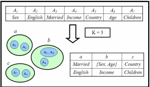
(29) CHAPTER 3 Clustering Composite Attributes In our approaches, we would like to solve the problem of attribute composition and clustering at the same time. When an attribute is selected from a cluster, the classification performance may be improved if it is combined with other attributes. These attributes could then be grouped into a composite attribute. Thus, appropriate attribute composition may improve the clustering effect of attributes. Take Figure 3.1 as an example to illustrate the idea. In Figure 3.1, there are seven attributes A1 to A7 in a data set and the cluster number is 3. A possible solution is shown in Figure 3.1, in which the seven attributes are divided into three clusters. If A1 and A6 are combined together and can get a good performance, then it is better for them to be a composite attribute.. The problem is thus stated as follows. Given a set of n attributes and a cluster number k, we would like to find appropriate attribute composition and cluster the single and composite attributes into k clusters, such that the evaluation criteria are (nearly) best satisfied. We will state the evaluation criterion later.. 17.

(30) Figure 3.1: An example for attribute composition and clustering. In Figure 3.1, the two attributes A1 and A6 in the second cluster are combined into a composite attribute. A feature set can then be formed with a single or composite attribute from each cluster. For example, A2, A4 and A5 can be chosen as a feature set. A2, (A1, A6) and A7 can also be chosen as another feature set. It can be seen from the example that the results in this way are more flexible than those without considering composite attributes. The example is also different from clustering four clusters in that it is mainly for three clusters and performs attribute substitution based on the three clusters instead of four.. Some evaluation criteria must thus be designed to evaluate the results. In the first approach, we will consider three factors, including average accuracy, cluster balance, and composition penalty. In the second approach, we will consider the center’s 18.

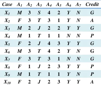
(31) accuracy, attribute similarity, cluster balance, and the average composition penalty for all possible feature subsets. The cluster balance and the attribute similarity will be described in CHAPTER 4 and 5, respectively. The accuracy and the composition penalty are stated below.. 3.1 Accuracy The first measure in the proposed approach is the accuracy, which is similar to that in Hong and Wang’s approach [17][18], but with a consideration of composite attributes. A single or a composite attribute is selected from a cluster, and all the attributes gathered together form a possible feature subset. The accuracy of the feature subset is then evaluated as follows. When the feature subset is used to classify training data, if the values of the features are all the same for some objects but the objects belong to different classes, then the correctly classified objects are defined as those belonging to the class with the maximum number of objects. The accuracy is then defined as the number of all the correctly classified objects divided by the number of all the objects considered. For example, assume a feature subset is (A4, A7), A1 and A6, where (A4, A7) is a composite attribute. Also assume the three objects, Obj1, Obj2 and Obj3, have the same values of these features. If the class of both Obj1 and Obj2 are 1 and that of Obj3 19.

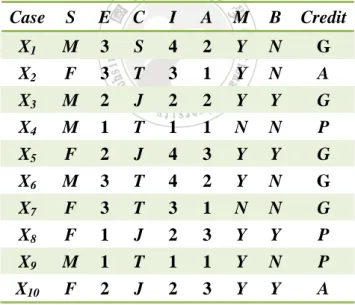
(32) are 0, then the classification by the feature values for Obj3 is considered wrong. If there are totally ten objects in a dataset, and the feature set can correctly classify seven objects among them, then the accuracy for the selected feature subset is 0.7. Below, an example is given to illustrate the concept.. Example 3.1: Table 3.1 shows a training example dataset U with 7 attributes and 10 objects. Assume {(A4, A7), A1, A6} is a possible feature subset. The attribute values of {(A4, A7), A1, A6} for X8 and X10 are {(2, F), Y, Y}, but the class for X8 and X10 are not the same. Therefore, one of the two classification results is thought of as wrong. Since the feature subset, {(A4, A7), A1, A6}, can correctly classify 9 objects for the dataset, its accuracy is thus 0.9.. Table 3.1: A training example dataset U with 7 attributes and 10 objects Case A1 A2 A3 A4 A5 A6 A7 Credit X1. M. 3. S. 4. 2. Y. N. G. X2 X3 X4 X5 X6 X7 X8 X9 X10. F M M F M F F M F. 3 2 1 2 3 3 1 1 2. T J T J T T J T J. 3 2 1 4 4 3 2 1 2. 1 2 1 3 2 1 3 1 3. Y Y N Y Y N Y Y Y. N Y N Y N N Y N Y. A G P G. 20. G G P P A.

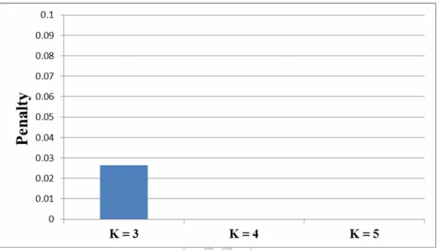
(33) 3.2 Composition Penalty The more attributes in a composite attribute, the higher accuracy for classification with the composite attribute. But the purpose of feature selection is to use less attributes to do classification. Thus some penalty should be given to composite attributes. A composite attribute with more attributes will be given more penalty. In this thesis, we use the following penalty function for a composite attribute A with x attributes:. 0 , if N = 1 ⎧ ⎪ Penalty( A) = ⎨⎛ x − 1 ⎞1+γ ………………… (2) ⎪⎜ N − 1 ⎟ , if N > 1 ⎠ ⎩⎝ where N is the number of all attributes and γ (0 ≤ γ ≤ 1) is a parameter to adjust the penalty curve. For example, the plot of the penalty function with γ = 0.5 is shown in Figure 3.2.. The penalty function has two properties. Firstly, the penalty is among 0 to 1. Secondly, the sum of the penalty values of two composite attributes respectively with x1 and x2 (x1 + x2 ≤ N) individual attributes will be smaller than that of the composite attribute with x1+x2 attributes. This is because a composite attribute with more attributes will be less desired. A single attribute can be thought of as a composite 21.

(34) attribute with only one attribute. In this case, the penalty is zero, which means no penalty. On the contrary, if a composite attribute includes all the N attributes, the penalty will be 1.. Figure 3.2: The plot of the penalty function with N = 8 and γ = 0.5. 22.

(35) CHAPTER 4 GA-Based Clustering for Composite Attributes In this chapter, a GA-based feature clustering algorithm for composite attributes is proposed. In this algorithm, we encode a possible composition and clustering result into a chromosome, and uses GA to drive the best one. The fitness of each chromosome is evaluated by the average accuracy of the possible attribute substitution in clusters, the cluster balance, and the total composition penalty for each possible feature subset.. 4.1 Chromosome Representation Each gene in a chromosome represents the status of an attribute, which can be divided into two parts, the composition part and the cluster part. The composition part is used to represent with which attributes an attribute can be combined into a composite attribute, and the cluster part is used to denote which cluster an attribute is located in. For convenient discussion, positive integers are used to encode the composition part and English lowercase letters to encode the cluster part. Assume. 23.

(36) there are n attributes, A1 to An, to be processed. In a chromosome, two attributes Ai to Aj with the same integer in the composition part will compose a composite attribute, and those with the same English lowercase letter will be located in the same cluster. Since the attributes composing a composite attribute have to be in the same cluster, the constraint that the letters should be the same for the genes with the same integers needs to be obeyed. An example is given below to illustrate it.. Example 4.1: Assume there are seven attributes {a1, a2, …, a7} to be divided into three clusters. Thus, K = 3 and N = 7. Suppose there is a chromosome shown in Table 4.1. According to its coding representation, A6 and A7 belong to cluster a, A1 and A4 belong to cluster b, and A2, A3 and A5 belong to cluster c. Besides, A3 and A5 compose a composite attribute and they have to be in the same cluster. Table 4.1: An example for chromosome representation A1. A2. A3. A4. A5. A6. A7. 1. 2. 3. 4. 3. 5. 6. b. c. c. b. c. a. a. 4.2 Initial Population Before the genetic algorithm begins, a set of P individuals are randomly generated to form the initial population. The composition part of a gene is 24.

(37) probabilistically set to a number among 1 to N, where N is the number of attributes. The probability for setting a larger composite attribute will be less than that for setting a smaller one. For example, composite attributes with 2 features will appear in the initial population with a higher probability than those with three attributes. Besides, single attributes will have a higher probability than composite attributes.. The cluster part of a gene is randomly set to a number among 1 to K, where K is the number of clusters. The probability distribution is like a normal distribution, with the total attribute number N divided by K (N/K) at the peak.. 4.3 Fitness and Selection In order to develop a good result of attribute clustering from an initial population, the proposed algorithm selects parent chromosomes with high fitness values for mating. A good evaluation (fitness) function is thus needed to achieve the purpose. The proposed fitness function consists of three factors: cluster accuracy, cluster balance and the total composition penalty. They are described as follows.. The cluster accuracy is used to evaluate the accuracy of a possible clustering result on the given training data. Since one purpose of the proposed 25.

(38) attribute-clustering approach is to reduce the adopted attribute number in approximate reasoning, a reasonable criterion for clustering results is thus the average accuracy of each attribute combination, which is composed of a single or composite attribute from each cluster. Take the chromosome in Figure 3.1 as an example. There are three clusters, with attributes A2 and A3 belonging to the first cluster, A4 and (A1 , A6) to the second cluster, and A5 and A7 to the third cluster. Note that (A1, A6) is a composite attribute. The number of all possible attribute combinations from the chromosome is then 2*2*2, which is 8.. Therefore for K clusters, one single or composite attribute from each cluster is selected and all the K selected attributes gathered together form a possible feature subset. Consider all the possible combinations from a chromosome. If all the combinations are of high accuracy, then any single or composite attribute in each cluster can be chosen to form the possible feature subset. That means the clustering result is good for classification. In this case, if an attribute value of a new data is missing or unavailable due to cost, it can be easily replaced with another single or composite attribute in the same cluster for classification. The replaced attribute subset can be expected to have a high accuracy for classification as well if the clustering result is good. The average accuracy of all the possible attribute combinations in a 26.

(39) chromosome thus provides a reasonable measure for its goodness.. For each combination, it is formed by some single or composite attributes. However, if there are some composite attributes in the combination, the number of attributes for the combination is larger than K. But the purpose of feature selection is to use less attributes to do classification. Thus some penalty should be given to composite attributes. All the composite attributes have their penalty, which is defined in Chapter 3. The penalty values will be summed into a total_penalty value to be another evaluation criterion.. Another evaluation criterion for the goodness of a clustering result is the cluster balance. When we divide the attributes into K clusters, we hope to cluster the attributes as balanced as possible. If a clustering result is unbalanced, a new object with missing values may not be classified since no other alternative attributes can be used in the single-attribute clusters. A simple example is given below. Assume there are two chromosomes, with their results shown in Figure 4.1 and Figure 4.2, respectively. The one in Figure 4.1 are more balanced than that in Figure 4.2 although the latter may have a better accuracy than the former.. 27.

(40) Figure 4.1: A more-balanced clustering result. Figure 4.2: A less-balanced clustering result. In Figure 4.2, a new object with a missing value in any of the two attributes, A3 and A6, can not be classified since no other alternative attributes can be used for 28.

(41) substitution.. The factor of cluster balance is thus important and designed here to avoid the above unbalanced situation. Formally, the factor of the cluster balance for a chromosome C is defined as follows: K. balance(C ) = ∑ − i =1. | clusteri | | clusteri | log , ………….. (3) CM CM. where |clusteri| represents the attribute number in the i-th cluster, and CM is the number of composite and single attributes, which may be less than the total number of attributes N. The measure of cluster balance is mainly based on the principle of entropy. If a clustering result is more balanced, then its value will be larger. For example, we may compare Figure 4.1 and Figure 4.2, in which CM is 6. The numbers of the composite attributes in the three clusters in Figure 4.1 are all 2, and those in Figure 4.2 are 1, 1 and 4, respectively. According to the above formula, the cluster balance for Figure 4.1 is 1.585 and for Figure 4.2 is 1.252. Therefore, the clustering results in Figure 4.1 are better.. According to the above three criteria - accuracy, cluster balance, and composition penalty, a fitness function can be designed to evaluate the goodness of 29.

(42) chromosomes as follows:. ⎛ |S | ⎜ (∑ (accuracyi * (1 − total _ penaltyi )α ) / | S | *balance(C ) β fitness(C ) = ⎜ i =1 ⎜ K − | Cluster (C ) | +1 ⎜ ⎝. ⎞ ⎟ ⎟, ⎟ ….. (4) ⎟ ⎠. where S is the set of all possible feature subsets from the clusters represented by the chromosome C, |S| is its cardinality, accuracyi is the classification accuracy of the i-th feature subset in S for a set of training examples, total_penaltyi is the total penalty of the composite attributes in the i-th feature subset, balance(C) is the cluster balance of the chromosome C, α and β are two parameters to adjust the relative importance of the three criteria, K is the given cluster number, and |Cluster(C)| is the actual cluster number of the chromosome C. Ideally, all the attributes should be divided into K clusters for a given K. But in some chromosomes, the clustering results may be less than K clusters, so some clustering penalty is given to avoid its occurrence. The denominator K-|Cluster(C)|+1 in the above formula can thus be regarded as the penalty for this situation. If in a chromosome C, all the attributes are divided into K clusters, then the result of K-|Cluster(C)|+1 becomes 1, meaning no penalty on the fitness evaluation. On the contrary, if the actual cluster number of a chromosome C is less than K, then the result of K-|Cluster(C)|+1 is at least 2 and the fitness value will become smaller than that for the actual cluster number being K. 30.

(43) Take the clustering results in Figure 4.2 as an example to illustrate the above fitness evaluation. From Figure 4.2, the following four feasible feature subsets can be obtained: {3, (1, 4), 6}, {3, 2, 6}, {3, 5, 6} and {3, 7, 6}. If γ = 0.05, the total penalty of the feature subset {3, (1, 4), 6} is calculates as [(1-1)/(7-1)]1.05 + [(2-1)/(7-1)]1.05 + [(1-1)/(7-1)]1.05, which is 0 + 0.152 + 0 (= 0.152). The total penalty for the other combinations can be similarly found. The accuracy of each feature subset is then evaluated based on the given training set. At last, the whole cluster balance of the clustering results is calculated according to the formula in above. For example, the accuracy values of the above feature subsets for the Table 3.1 are 0.9, 0.8, 0.6 and 0.5, respectively, and the cluster balance is calculated as 1.252. After that, the fitness of the chromosome representing the clustering results in Figure 4.2 can be obtained. Assume both α and β are 1. The value of |Cluster(C)| is 3, and the fitness of the clustering results in Figure 4.2 is 0.834.. The fitness values of the chromosomes will be used for selecting individuals to execute crossover, mutation and reproduction. If an individual has a higher fitness value, it will be selected with a higher probability. Different probabilities control different mixed ratios from the parents. Each parent will be selected according to 31.

(44) roulette wheel selection strategy for crossover with a crossover rate Pc.. 4.4 Genetic Operators Genetic operators are very important to the success of specific GA applications. Two important genetic operators in GAs are crossover and mutation. The crossover operator is first introduced here. It selects pairs of individuals from the current population for crossover. In the paper, the uniform crossover is used in the proposed genetic attribute-clustering approach. For the uniform crossover operator, a mask sequence is randomly generated for each pair to decide which genes will be exchanged. A mask sequence is composed of binary bits, with ‘1’ represents the corresponding attributes of the pair of chromosomes will exchange their gene values and ‘0’ representing no exchange. The following three kinds of crossovers will be executed. 1. Only the composition part exchanges according to the mask sequence. The cluster part will remain unchanged no matter what the mask sequence is. 2. Only the cluster part exchanges according to the mask sequence. The composition part will remain unchanged no matter what the mask sequence is. 3. Both the composition part and the cluster part exchange according to the mask sequence. 32.

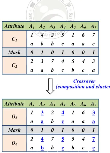
(45) Thus, six children will be generated from a pair of chromosomes, and then the best two among them are chosen for competition with the ones from other pairs of chromosome by the reproduction procedure to survive in the next generation. Below, an example is given to show the process of the crossover operation. Assume there are two chromosomes C1 and C2 shown as in Table4.2.. Table 4.2: Two chromosomes for crossover Attribute A1 A2 A3 A4 A5 A6 A7 C1 C2. 1. 4. 2. 5. 1. 6. 7. a. b. b. c. a. a. c. 2. 3. 7. 4. 5. 4. 3. a. a. b. c. b. c. a. Also assume the mask sequence for the pair of chromosomes is randomly generated as shown in Table 4.3.. Table 4.3: The mask sequence in the example 0. 1. 0. 1. 0. 0. 1. The three crossover operations are then executed on C1 and C2 according to the mask sequence. For the first kind of crossover operation, only the composition part 33.

(46) exchanges according to the mask sequence. The results are shown in Figure 4.3.. Attribute A1 A2 A3 A4 A5 A6 A7 C1 Mask C2. 1. 4. 2. 5. 1. 6. 7. a. b. b. c. a. a. c. 0. 1. 0. 1. 0. 0. 1. 2. 3. 7. 4. 5. 4. 3. a. a. b. c. b. c. a. Crossover (composition) Attribute A1 A2 A3 A4 A5 A6 A7 O1 Mask O2. 1. 3. 2. 4. 1. 6. 3. a. b. b. c. a. a. c. 0. 1. 0. 1. 0. 0. 1. 2. 4. 7. 5. 5. 4. 7. a. a. b. c. b. c. a. Figure 4.3: The results after the first kind of crossover. In Figure 4.3, A2,A4 and A7 in C1 and C2 exchange the composition part of their gene values. Since the attributes A2 and A7 within the composite attribute with the composition number 3 belong to different classes, their clusters have to be adjusted to be the same. In this example, the cluster of A7 in O1 is adjusted from c to b. The cluster adjustment process will be introduced later. The results are then shown in Table 4.4. The clusters of A2 and A7 thus become identical. Similarly, the clusters of A5, A6 and A7 in O2 is changed to c, a and b, respectively. 34.

(47) Table 4.4: The results after the adjustment for the first kind of crossover operation Attribute A1 A2 A3 A4 A5 A6 A7 O1 O2. 1. 3. 2. 4. 1. 6. 3. a. b. b. c. a. a. b. 2. 4. 7. 5. 5. 4. 7. a. a. b. c. c. a. b. For the second kind of crossover operation, only the cluster part exchanges according to the mask sequence. The results are shown in Figure 4.4.. Attribute A1 A2 A3 A4 A5 A6 A7 C1 Mask C2. 1. 4. 2. 5. 1. 6. 7. a. b. b. c. a. a. c. 0. 1. 0. 1. 0. 0. 1. 2. 3. 7. 4. 5. 4. 3. a. a. b. c. b. c. a. Crossover (cluster) Attribute A1 A2 A3 A4 A5 A6 A7 O3 Mask O4. 1. 4. 2. 5. 1. 6. 7. a. a. b. c. a. a. a. 0. 1. 0. 1. 0. 0. 1. 2. 3. 7. 4. 5. 4. 3. a. b. b. c. b. c. c. Figure 4.4: The results after the second kind of crossover. Again, the adjustment process has to be done to make the composite attributes. 35.

(48) consistent in their cluster numbers. The results after the adjustment process are shown in Table 4.5. Table 4.5: The results after the adjustment for the second kind of crossover operation Attribute A1 A2 A3 A4 A5 A6 A7 O3 O4. 1. 4. 2. 5. 1. 6. 7. a. a. b. c. a. a. a. 2. 3. 7. 4. 5. 4. 3. a. b. b. c. b. c. b. At last, for the third kind of crossover operation, both the composition and the cluster parts exchange according to the mask sequence. The results are shown in Figure 4.5. Attribute A1 A2 A3 A4 A5 A6 A7 C1 Mask C2. 1. 4. 2. 5. 1. 6. 7. a. b. b. c. a. a. c. 0. 1. 0. 1. 0. 0. 1. 2. 3. 7. 4. 5. 4. 3. a. a. b. c. b. c. a. Crossover (composition and cluster) Attribute A1 A2 A3 A4 A5 A6 A7 O5 Mask O6. 1. 3. 2. 4. 1. 6. 3. a. a. b. c. a. a. a. 0. 1. 0. 1. 0. 0. 1. 2. 4. 7. 5. 5. 4. 7. a. b. b. c. b. c. c. Figure 4.5: The results after the third kind of crossover 36.

(49) Again, the adjustment process has to be done to make the composite attributes consistent in their cluster numbers. The results after the adjustment process are shown in Table 4.6.. Table 4.6: The results after the adjustment for the third kind of crossover operation Attribute A1 A2 A3 A4 A5 A6 A7 O5 O6. 1. 3. 2. 4. 1. 6. 3. a. a. b. c. a. a. a. 2. 4. 7. 5. 5. 4. 7. a. b. b. c. c. b. b. Six children are thus generated from the pair of chromosomes C1 and C2. Then the fitness values of the six children are evaluated and the best two of them are kept for competition.. The mutation operation is executed after the crossover is done. It is performed on single chromosomes, instead of pairs of chromosomes as in crossover. The multi-point operation is the most commonly used among the mutation operations. It decides a gene in a chromosome for mutation according to a low mutation probability Pm. In the proposed representation, each gene includes two parts, the composition part 37.

(50) and the cluster part. The one point mutation operation is then modified as selecting a part of a gene in a chromosome for mutation. If the composition part of a gene is selected, it is randomly reset to a number among 1 to N, where N is the number of attributes. If the cluster part of a gene is selected, it is randomly reset to a number among 1 to K, where K is the number of clusters. Appropriate cluster adjustment process may need to be done as well after the mutation operation. An example is given in Figure 4.6 to illustrate the mutation process, in which A3 is selected to mutate for the composition part (from 2 to 3) and A6 is selected for the clustering part (from a to b).. Attribute A1 A2 A3 A4 A5 A6 A7 O5. 1. 3. 2. 4. 1. 6. 3. a. a. b. c. a. a. a. Mutation Attribute A1 A2 A3 A4 A5 A6 A7 O5. 1. 3. 3. 4. 1. 6. 3. a. a. b. c. a. b. a. Figure 4.6: The results after the mutation. After the mutation, the resulting chromosome has to be adjusted to make the composite attributes consistent with their cluster numbers. In this example, the cluster number of A3 is changed from b to a to make the composite attribute consistent with 38.

(51) the cluster numbers of its components. The results after the adjustment process are shown in Table 4.7.. Table 4.7: The results after the adjustment Attribute A1 A2 A3 A4 A5 A6 A7 O5. 1. 3. 3. 4. 1. 6. 3. a. a. a. c. a. b. a. After crossover and mutation, some offspring chromosomes are generated. A selection mechanism “roulette wheel selection” is then adopted to form the population in the next generation. The above process is then repeated again until some termination criteria are satisfied. The criteria may include number of generations, execution time, or convergence of solutions obtained.. 4.5 Cluster Adjustment As mentioned above, the cluster adjustment process may need to be done after crossover and mutation operations. It is mainly used for avoiding the situation that the components in a composite attribute belong to different clusters, thus causing inconsistency. The process acts in the following way. If the cluster parts of the genes belonging to a certain composite attribute are not the same (with different English 39.

(52) lower-case letters), then the process is activated. It first finds out the cluster with the maximum occurrence number among the components of the composite attribute, and then reset the other clusters in the composite attribute to it. For example, assume a composite attribute includes three attributes, A1, A4 and A7 with their cluster parts being c, a and c, respectively. The cluster part of A4, which is originally a, will be reset to c.. If more than one cluster within a certain composite attributes have the same maximum occurrence number, then a cluster will be randomly generated from them. For the above example, assume the three attributes, A1, A4 and A7, have their cluster parts as a, b and c respectively, then a cluster among the set {a, b, c} will be randomly chosen. Assume the cluster b is chosen in the example. The cluster parts of the other two attributes A1 and A7 (originally a and c) will be adjusted to b. After the adjustment process, it can be guaranteed that the components within a composite attribute will be located in the same cluster. A simple example is given below to illustrate the idea.. Example 4.2: In Figure 4.7, A2, A3 and A7 is a composite attribute, but the cluster parts are not the same. The cluster adjustment process is then executed. The cluster part of A2 and A3 are ‘a’, and the cluster part of A7 is ‘b’. The cluster with the 40.

(53) maximum occurrence number is thus ‘a’, and we reset ‘b’ to ‘a’. In Figure 4.8, A1 and A5 is a composite attribute, but their cluster parts are not the same. The cluster part of A1 is ‘a’, and of A5 is ‘c’. The cluster with the maximum occurrence number is ‘a’ or ‘c’. Therefore, we randomly choose one from them and reset the other. In Figure 4.8, the cluster part of A1 is reset from ‘a’ to ‘c’.. Attribute A1 A2 A3 A4 A5 A6 A7 O5. 1. 3. 3. 4. 1. 6. 3. a. a. a. c. A. b. b. Attribute A1 A2 A3 A4 A5 A6 A7 O5. 1. 3. 3. 4. 1. 6. 3. a. a. a. c. A. b. a. Figure 4.7: An example for the adjustment process. Attribute A1 A2 A3 A4 A5 A6 A7 O5. 1. 3. 3. 4. 1. 6. 3. a. a. a. c. c. b. a. Attribute A1 A2 A3 A4 A5 A6 A7 O5. 1. 3. 3. 4. 1. 6. 3. c. a. a. c. c. b. a. Figure 4.8: An example in the adjustment process with a tie. 41.

(54) 4.6 The Proposed Algorithm According to the above description, the proposed GA-based algorithm for composite-attribute clustering is described below.. The proposed algorithm for clustering composite attributes: INPUT: A training dataset with N attributes and a cluster number K. OUTPUT: An appropriate K clusters of single or composite attributes. STEP 1: Generate an initial population of P individuals (chromosomes) randomly, with each being a feasible attribute clustering result. STEP 2: Calculate the fitness value of each chromosome C by the following sub-steps. STEP 2.1: Determine all the possible feature subsets from the clustering results represented by the chromosome C. STEP 2.2: Determine the accuracy of each possible feature subset from the given training examples. STEP 2.3: Calculate the total penalty of each possible feature subset according to the component numbers of the composite attributes in the feature subset. STEP 2.4: Calculate the cluster balance of the chromosome Ci according to 42.

(55) Formula (3) mentioned in Chapter 4.3. STEP 2.5: Calculate K-|Cluster(C)|+1, where |Cluster(C)| is the number of clusters for chromosome C. STEP 2.6: Calculate the fitness value of the chromosome according to Formula (4) mentioned in Chapter 4.3. STEP 3: Execute the crossover operations according to the fitness values of the chromosomes and the crossover rate Pc. STEP 4: Execute the mutation operations according to the mutation rate Pm. STEP 5: Execute the cluster adjustment for the offspring generated. STEP 6: Calculate the fitness value of the chromosomes in the adjusted offspring by the same procedure of Step 2. STEP 7: Generate the next generation according to the roulette wheel selection strategy. STEP 8: If the termination criterion is not satisfied, go to Step 3; otherwise, do the next step. STEP 9: Output the chromosome with the best fitness value to users.. After Step 9, an appropriate composite-attribute clustering result about which attributes will compose the composite attributes and which attributes will be grouped 43.

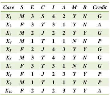
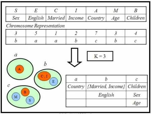
(56) together is obtained. After that, any single or composite attribute can be chosen from each cluster and all the chosen attributes gathered together form a promising feature subset. In this way, the problem of missing attribute values could be partially solved since it can replace an attribute with missing values by another attribute in the same cluster.. 4.7 An Example In this section, an example is given to illustrate the proposed genetic composite attribute-clustering algorithm. Assume there are ten objects with the seven attributes: Sex (S), English (E), Country (C), Income (I), Age (A), Married (M), Buying Computer (B). The class name is Credit. The database is shown in 0 4.8.. Table 4.8: Ten objects in the example Case. S. E. C. I. A. M. B. Credit. X1 X2 X3 X4 X5 X6 X7 X8 X9 X10. M F M M F M F F M F. 3 3 2 1 2 3 3 1 1 2. S T J T J T T J T J. 4 3 2 1 4 4 3 2 1 2. 2 1 2 1 3 2 1 3 1 3. Y Y Y N Y Y N Y Y Y. N N Y N Y N N Y N Y. G A G P G. 44. G G P P A.

(57) For the data shown in Table 4.8, the proposed algorithm proceeds as follows:. STEP 1: Generate P individuals randomly as the initial population. In this example, assume P is set at 4 and K = 3. Each individual represents a possible clustering result. Assume the four initial chromosomes are generated as shown in 0 4.9. Table 4.9: The four initial chromosomes. ID C1 C2 C3 C4. S. Chromosome E C I A. M. B. 4. 2. 1. 5. 2. 3. 5. a. a. a. c. a. b. c. 1. 1. 5. 2. 4. 3. 1. a. a. c. a. b. b. a. 3. 2. 5. 6. 4. 7. 1. c. c. c. c. c. c. a. 3. 3. 4. 5. 6. 1. 2. b. b. a. b. a. c. a. STEP 2: The fitness value of each chromosome is calculated by the following sub-steps.. STEP 2.1: Find all the possible attribute combination from the clustering result. Take the first chromosome C1 as an example. It includes the following 3 combinations: {S, M, (I, B)}, {(E, A), M, (I, B)} and {C, M, (I, B)}. 45.

(58) STEP 2.2: The accuracy of each possible attribute combination is calculated. Take the first chromosome C1 as an example. The accuracy values of the three possible attribute combinations for the training dataset are evaluated as 0.8, 1 and 0.9, respectively.. STEP 2.3: The total penalty of each possible attribute combination is calculated. Take the first chromosome C1 as an example. If the parameter γ was set at 0.05, then the total penalty values of the three possible attribute combinations are calculated as follows: {S, M, (I, B)}: [(1-1)/(7-1)]1.05 + [(1-1)/(7-1)]1.05 + [(2-1) / (7-1)]1.05 = 0.152, {(E, A), M, (I, B)}: [(2-1)/(7-1)]1.05 + [(1-1)/(7-1)]1.05 + [(2-1) / (7-1)]1.05 = 0.305, {C, M, (I, B)}: [(1-1)/(7-1)]1.05 + [(1-1)/(7-1)]1.05 + [(2-1) / (7-1)]1.05 = 0.152.. STEP 2.4: The cluster balance of each chromosome is calculated according to Formula (3). Again, take the first chromosome C1 as an example. It has 3, 1 and 1 single or composite attributes in the three clusters. Its value of cluster balance is then calculated as follows:. 3 1 1 1 1 balance (C1 ) = − * log 3 − * log − * log = 1.371. 5 5 5 5 5 46.

(59) STEP 2.5: Calculate K-|Cluster(C)|+1, where |Cluster(C)| is the number of clusters for chromosome C. Here, |Cluster(C1)| of the chromosome C1 is 3, and the result is 3-3+1, which is 1.. STEP 2.6: The fitness value of each chromosome is calculated according to Formula (4). Take the chromosome C1 as an example. Let the parameter α and β are all set at 1. Its accuracy and total penalty values of the 3 possible attribute combinations are {0.8, 1, 0.9} and {0.152, 0.305, 0.152}. Its cluster balance is 1.371. The fitness value of C1 is then calculated as follows:. 1 [0.8 * (1 − 0.152)1 + 1 * (1 − 0.305)1 + 0.9 * (1 − 0.152)1 ] *1.3711 f (C1 ) = 3 = 0.976. 1. The fitness values of all the chromosomes in Table 4.9 are shown in Table 4.10.. Table 4.10: The fitness values of all the chromosomes in the example Chromosome. Fitness Value. C1 C2 C3. 0.976 1.052 0.178 1.165. C4 47.

(60) STEP 3: Execute the crossover operations on the population. Assume the two chromosomes C1 and C2 are selected for crossover. Also assume the mask sequence is randomly set at {1, 0, 0, 1, 1, 0, 1}. The six offspring chromosomes O1 to O6 for the three kinds of crossover operations are generated from the two parents as shown in Figure 4.9. O1 and O2 are generated by the first kind of crossover operation, O3 and O4 are the second kind, and O5 and O6 are third kind.. 4. 2. 1. 5. 2. 3. 5. a. a. a. c. a. b. c. 1. 1. 5. 2. 4. 3. 1. a. a. c. a. b. b. a. 4. 1. 5. 5. 2. 3. 5. a. a. c. a. b. b. a. 1. 1. 5. 2. 4. 3. 1. a. a. c. c. a. b. c. 4. 1. 5. 5. 2. 3. 5. a. a. c. c. a. b. c. C1:. C2:. O1 O3 O5. 1. 2. 1. 2. 4. 3. 1. a. a. a. c. a. b. c. 4. 2. 1. 5. 2. 3. 5. a. a. a. a. b. b. a. 1. 2. 1. 2. 4. 3. 1. a. a. a. a. b. b. a. O2 O4 O6. Figure 4.9: The six offspring for the three kinds of crossover by C1 and C2. The six offspring chromosomes are then adjusted through the cluster adjustment process. The results after the cluster adjustment are shown in Figure 4.10. 48.

(61) O1 O3 O5. 1. 2. 1. 2. 4. 3. 1. a. c. a. c. a. b. a. 4. 2. 1. 5. 2. 3. 5. a. b. a. a. b. b. a. 1. 2. 1. 2. 4. 3. 1. a. a. a. a. b. b. a. O2 O4 O6. 4. 1. 5. 5. 2. 3. 5. a. a. a. a. b. b. a. 1. 1. 5. 2. 4. 3. 1. a. a. c. c. a. b. a. 4. 1. 5. 5. 2. 3. 5. a. a. c. c. a. b. c. Figure 4.10: The six offspring chromosomes after the cluster adjustment. STEP 4: The mutation operator is executed with a low probability Pm to generate possible offspring. The operation is similar to the traditional one. Take O1 in Figure 4.11 as an example. Its resulting chromosome is O1’. Assume the results of the six offspring chromosomes after mutation are shown in Figure 4.12. 1. 2. 1. 2. 4. 3. 1. a. c. a. c. a. b. a. O1:. Mutation 1. 2. 1. 2. 4. 5. 1. a. b. a. c. a. b. a. O1’:. Figure 4.11: The offspring of O1 after the mutation operation O1’ O3’ O5’. 1. 2. 1. 2. 4. 5. 1. a. b. a. c. a. b. a. 4. 2. 1. 5. 2. 3. 5. a. b. a. a. c. b. a. 1. 2. 1. 2. 4. 3. 1. a. a. a. a. b. b. a. O2’ O4’ O6’. 4. 1. 5. 7. 2. 3. 5. a. a. a. a. b. b. a. 1. 1. 6. 2. 2. 3. 1. a. a. c. c. a. b. a. 4. 1. 5. 5. 2. 3. 5. a. a. b. c. b. b. c. Figure 4.12: The six offspring chromosomes after the mutation operation 49.

(62) STEP 5: Execute the cluster adjustment process if the cluster parts of a composite attribute are not the same after crossover and mutation operations. Take the offspring O1’ as an example. The result after adjustment is illustrated in Figure 4.13. The results of the six offspring chromosomes after the cluster adjustment are shown in Figure 4.14.. 1. 2. 1. 2. 4. 5. 1. a. b. a. c. a. b. a. O1’:. Cluster Adjustment 1. 2. 1. 2. 4. 5. 1. a. c. a. c. a. b. a. O1’:. Figure 4.13: The offspring O1 ' after the cluster adjustment.. O1’ O3’ O5’. 1. 2. 1. 2. 4. 5. 1. a. c. a. c. a. b. a. 4. 2. 1. 5. 2. 3. 5. a. c. a. a. c. b. a. 1. 2. 1. 2. 4. 3. 1. a. a. a. a. b. b. a. O2’ O4’ O6’. 4. 1. 5. 7. 2. 3. 5. a. a. a. a. b. b. a. 1. 1. 6. 2. 2. 3. 1. a. a. c. a. a. b. a. 4. 1. 5. 5. 2. 3. 5. a. a. c. c. b. b. c. Figure 4.14: The six offspring chromosomes after the cluster adjustment.. 50.

(63) STEPs 6 to 9: The best two offspring chromosomes are then selected for competing with others for the next generation. The same procedure is then executed until the termination criterion is satisfied. The best chromosome with the highest fitness value is then output as the clustering result.. After step 9, an appropriate composite-attribute clustering result is obtained, and the clustering result can then be flexibly used for classification.. 51.