Willingness to Pay and the Demand for Lotto
Larry Y. Tzeng**
Jen-Hung Wang Jill Tain
Abstract
The literature has recognized that bettors may dislike risk but prefer positive skewness. The paper proposes a method to measure the willingness-to-pay for lotto, and provides a theoretical rationale for a bettor to participate in an unfair lottery. On basis of the predictions from willingness-to-pay, the paper further proposes an alternative model for empirical studies on the demand for lotto.
*
* Larry Y. Tzeng is a Professor of the Finance Department at National Taiwan University, Taiwan. Jen-Hung Wang is an Assistant Professor of the Finance Department at Shih Hsin University, Taiwan.
1. Introduction
The literature (Golec and Tamarkin, 1998; Garrett and Sobel, 1999; Woodland and Woodland, 1999) has recognized that bettors may dislike risk but prefer positive skewness. Golec and Tamarkin (1998) and Garrett and Sobel (1999) employed a cubic utility function to show betters may accept low-return, high-variance bets to exchange for positive skewness of the bets. However, both Golec and Tamarkin (1998) and Garrett and Sobel (1999) did not provide much economic justification for choosing a cubic utility function. To justify using the cubic utility function, Golec and Tamarkin (1998) argued that “Our alternative is to approximate u(xn). by a
Taylor series truncated to three terms and then to take expectation.” In this paper, we would like to follow the same approach suggested by Golec and Tamarkin (1998) to study the demand for lotto. We intend to show that expanding the utility function by Taylor series and truncating up to certain terms could be necessary to explain why the bettor participates in an unfair lotto. In other words, we propose that the utility function of bettors could be better characterized by a locally (but not globally) risk-averse function. We further use the willingness-to-pay for lotto to justify the empirical approach for choosing a cubic utility function and to provide theoretical rationale for empirical findings both in the literature and in this paper.
Woodland (1999) used data from horse track betting, lottery games and baseball bets. We choose to study data from lottery games because the lottery is the most popular form of gambling in the whole world. The second goal of the paper is to provide an alternative empirical model for the demand for lotto.
The most popular empirical model for the demand for lotto is the so-called “effective price” approach (Cook and Clotfelter, 1993; Gulley and Scott, 1993; Scott and Gulley, 1995; Walker, 1998; Farrel et al., 1999; Purfield and Waldron, 1999; and Forrest et al., 2000). The effective price of a unit-value ticket is equivalent to one minus the expected value of the bet’s payoffs. Since the effective price cannot be observed ex ante, previous studies argued that bettors form their rational expectation of the effective price, using all available information such as previous sales, sales trends, and the amount of money carried over from the previous draws. However, we contend that the traditional “effective price” approach suffers by omitting important variables.
Most research using traditional “effective price” approach has two major drawbacks. First, no explanatory variable in regressors can explain why a bettor accepts an unfair gamble. Second, the estimation is biased if the model omits important variables. Thus, we intend to propose a modified model to estimate the demand for lotto.
Following our theoretical model developed below, we predict that the moments of the bets, including mean, variance, and third moment, play critical roles in an individual’s gambling decision. The traditional “effective price” approach only considers the first moment of the bet but ignores important variables such as variance and third moment. Therefore, for the empirical studies of the demand for lotto, we propose an alternative model which takes both the first and the higher moments of the bet into consideration.
This paper is organized as follows: Section 2 provides a theoretical model to measure willingness to pay for a lottery ticket, providing the rationale to explain why a bettor accepts an unfair gamble; and generate testable hypothesis. Section 3
proposes an alternative empirical model to estimate the demand for lotto. Section 4 describes our data and provides our empirical evidences. Section 5 concludes the paper.
2. A Model for Willingness to Pay
Assume that P and
x
denote the price and the (random) payoff of the lotto, respectively. Thus, an individual with initial wealth W is willing to purchase a lottery ticket if )] ( [ ) (W E u W P x u , (1)where
u
and E are respectively the underlying utility function and the expectation operator.Let
E(x)
P , (2)
where
is the extra (unfair) payment for the individual to purchase the lotto. Assume that
*
is the willingness-to-pay over the mean for the individual topurchase a lottery ticket and can be evaluated by
)] * ) ( ( [ ) (W E u W E x x u . (3)
Obviously, an individual is willing to purchase a lottery ticket if and only if
* . (4)
For a globally risk-averse utility function,
*
is less than zero. However, thisassumption conflicts to our observations that bettors do buy unfair lottery tickets. In the evidence, to justify why bettors accept unfair gamble, previous research argued that gambling could provide entertainment or bettors are risk-loving. Without any doubt, gambling could provide certain entertainment for some individuals. The problem is whether only the entertainment of the gamble can create this huge demand for lotto. On the other hand, if the individual buys an unfair lotto because he is risk-loving. It conflicts to our other observation, why he also buys unfair insurance. In our paper, to explain why bettors purchase unfair lotto, we propose that the bettors may be locally risk-averse but not globally.
To measure the willingness-to-pay for the lotto, we follow the approach used by Pratt (1964), modified in the following two ways. First, Pratt analyzed the behavior of willingness-to-pay for a risky asset with a small variance, whereas we do not assume that the variance of a lotto’s payoff is small. Second, Pratt assumed that the third absolute central moment of the random variable is of a smaller order than variance and, therefore, ignored the influence of moments of the random variable higher than variance. We will assume instead that the influence of some higher moments of the random variable can be ignored because the higher derivatives of an individual’s utility function are small enough.
Thus, by Taylor’s expansion around the initial wealth W, Equation (3) can be rewritten as ))} ( ( ) ( *) )] ( ([ ! 1 ) ( { ) ( () ( 1) 1 W u O W u x E x i W u E W u n i n i i
, (5)where the last term is expressed by the symbol “at most of the order …”. Equation (5) can be further expressed as
))] ( ( [ ) ( *) )] ( ([ ! 1 0 () ( 1) 1 W u O E W u x E x E i n i n i i
. (6)If, as we will assume, E[O(u(n1)(W))] can be ignored, then Equation (6) can
be rewritten as 0 ) ( *) )] ( ([ ! 1 () 1
W u x E x E i i n i i . (7)*
can be determined from Equation (7), though Equation (7) generally does not provide an explicit solution for
*
. Whence many insightful results can bederived.
Proposition 1
If n2 and if sign(u(i)(W))sign((1)i1),i 1, 2, no positive solution for
*
in Equation (7) exists.Proof
If n 1, then *0 obviously. If n2, then
in Equation (7) can be expressed as ) ( } *) ( )] ( [ { 2 1 ) ( *u(1) W E x E x 2 2 u(2) W . (8)Since u(1)(W)0 and u(2)(W)0,
in Equation (8) can never be equal to zero forany positive
*
.Q. E. D.
When n 1, the utility function is approximated by a linear function. Thus, the individual’s preference is characterized as risk neutral. Since a risk-neutral individual only cares about the expected value, he or she will pay no more than the expected
value for the lotto. Thus, as predicted by Proposition 1,
*
cannot be positive.If
n
,2
u
)1(
(
W
)
,0
u
(
)2
(
W
)
0
, the individual’s preference is characterizedby a mean-variance utility.1 In this case, the result of Proposition 2 is consistent with
a puzzle in the literature--individuals are willing to pay a significantly unfair amount of money to purchase a lottery ticket and at the same time purchase insurance to cover their other potential losses. Proposition 2 points out that this puzzle cannot be solved if the individual’s preference is characterized by a mean-variance utility function and the individual is risk averse. It should be recognized that, in such cases, there exists no solution for willingness-to-pay if the individual is assumed to exhibit local risk aversion. However, if the individual is locally risk loving, there might be a positive solution for willingness-to-pay in an unfair game.
Let us further discuss the case when n 3. Equation (7) can then be expressed as 0 ) ( ) * * 3 ( 6 1 ) ( ) * ( 2 1 ) ( * (1) 2 2 (2) 3 2 3 (3) u W x u W sx x u W , (9) where 2 E(x E(x))2 x and s3 E(x E(x))3 x .
1 It should be noticed that sign(u(i)(W)) sign((1)i1) are specified only at the initial wealth
Proposition 2 If ( ()( )) (( 1) 1), 1, ,3 sign i W u sign i i and if ( ) 0 6 1 ) ( 2 1 2u(2) W s3u(3) W x x ,
then there exists at least one positive solution for
*
in Equation (9).Proof
Under the conditions, ( )) 1
6 1 ( ) ( sign u(3) W sign , when *. On
the other hand, when *0, ( ) 0
6 1 ) ( 2 1 2 (2) 3 (3) xu W sxu W
. Thus, there exists
at least one positive solution for
*
in Equation (9).Q. E. D.
If, as assumed, u(2)(W)0 and u(3)(W)0, then 30
x s is a necessary condition for ( ) 0 6 1 ) ( 2 1 2u(2) W s3u(3) W x x
. The literature has recognized that
bettors prefer skewness but not risk. Proposition 2 confirms the empirical findings that a bettor is willing to pay an unfair amount of money for lotto only if the lotto provide a positive third moment large enough. Furthermore, if 3 0
x
condition ( ) 0 6 1 ) ( 2 1 2u(2) W s3u(3) W x x can be rewritten as 3 0 ) ( ) ( 3 2 ) 2 ( ) 3 ( x x s W u W u .
Thus, the individual must be prudent, i.e., with 0 ) ( ) ( ) 2 ( ) 3 ( W u W u . Proposition 2 shows
that u(3)(W)0 is a critical assumption for a bettor to purchase an unfair lottery
ticket.
Proposition 2 provides justification for previous empirical research, which assumed the utility function of the bettor is a cubic function. Moreover, Proposition 2 shows that, to make a bettor willing to purchase an unfair lottery ticket, the utility function of the bettor should be convex for a large gain. It is very important to recognize that risk aversion and prudence in Proposition 2 are defined locally not globally. If the utility function of the individual is assumed to be concave globally, then the individual may purchase unfair insurance (Mossin, 1968) but will never purchase an unfair lottery ticket. In Proposition 2, the utility function of the
individual is assumed to be concave locally but not globally. Thus, Proposition 2 may at least partially explain the puzzle that individuals purchase lotto tickets and
insurance at the same time. It is still rational for a locally risk-averse individual to purchase insurance. On basis of Proposition 2, when the lotto provides a large third moment, a locally risk-averse individual may also purchase the lotto ticket if his or
her prudence is higher than a certain level.
Proposition 3
Under the conditions of Proposition 2, we have
0
*
x
.0
*
xs
. Proof 0 ) ( ) * * 3 ( 6 1 ) ( ) * ( 2 1 ) ( * (1) 2 2 (2) 3 2 3 (3) u W x u W sx x u W , From Equation (9),0
)
(
)
*
(
2
1
)
(
*
)
(
*
) 3 ( 2 2 ) 2 ( ) 1 (
W
u
W
u
W
u
x
. 0 ) ( * ) ( (3) ) 2 ( W u W u x x x . 0 ) ( 2 1 2 (3) W u s s x x .Thus, by the implicit function theorem,
0
*
*
x x .0
*
*
x xs
s
. Q. E. D.Proposition 3 shows that a risk-averse and prudent bettor actually dislikes risk (standard deviation) but prefers standard third moment. The willingness-to-pay for the lotto is by definition equal to *E(x). From Proposition 3, if the standard deviation (respectively, standard third moment) of the lotto’s payoff increases, then the willingness-to-pay of the individual decreases (respectively, increases). It should also be recognized that the bettor prefers an increase in expected value, since the willingness-to-pay for the lotto is equal to *E(x).
Assume that the individual’s willingness-to-pay can be well-characterized by
Equation (9). Local risk aversion and prudence together imply
*
0
x
and0
*
xs
. Moreover, local prudence is a necessary condition to observe
*
0
x
and
*
0
xs
. Therefore, if we observe that bettor dislikes standard deviation and
prefers standard third moment, then the individual must be locally prudent, although he or she may or may not be locally risk averse. The empirical results in the next section show that demand for lotto decreases (increases) with respect to standard deviation (standard third moment) of the lotto, suggesting that bettors are locally prudent.
3. Empirical Models of Demand for Lotto
Traditionally, the effective price models to test demand for lotto typically use a two-stage regression. In the first stage, some observable variables, such as occurrence and the size of rollovers, are used as instruments to determine the effective price. In the second stage, demand for lotto is regressed on the effective price estimated in the first stage. The traditional model can be expressed as:
P p X
P 1 , in the first stage, and
Q P Q P
X
Q ˆ
2 , in the second stage. (11)
In Equation (11), P and Q are the effective price and the sales of lotto,
respectively. X1 and X2 are instrument and control variables and Pˆ is the
estimated effective price from the first stage regression . P, Q, and P are
estimated coefficients, while P and Q are residuals.
price cannot be observed ex ante. Thus, it is argued that bettors form their rational expectation of the effective price by using available information, such as previous sales, sales trends, and the amount of money carried over from the previous draws. Although the effective price model generally fits well in previous empirical studies, it does not explain why a bettor accepts an unfair game. To echo the theoretical predictions from the previous section and to answer the fundamental challenge in theory, we propose an alternative model for empirical studies as:
P p X
P 1 ,
Second Moment X1S S,
Third Moment X1T T in the first stage, and
S P Q P
X
Q ˆ
2 Standard Dˆeviation+T Standard Tˆhird Moment +
Q
,
in the second stage. (12)
In Equation (12), Second Moment and Third Moment are the second and third moments of the lotto. Standard Dˆeviation and StandardTˆhird Moment are the estimated standard deviation and standard third moment from the first stage; s and
T
are residuals.
Had we directly put Second Moment and Third Moment, which is estimated from the first stage, into the second stage regression, the rank condition would be violated. The coefficients of regression would not be unique as the explanatory
variables were linearly dependent, and the data matrix were not of full rank. The following technique is used to avoid this problem. First we get Second Moment and Third Momentin the first stage, (P, S, T are estimated
coefficients in the first regression). We then define StandardTˆhird Moment as the cubic root of the estimated Third Moment and Standard Dˆeviation as the square root of the estimated Second Moment. We will use Standard Dˆeviation and
Moment hird
T dard
Stan ˆ as explanatory variables in the second stage to overcome
the problem of multicollinearity. Besides, it is more reasonable to use eviation
D dard
Stan ˆ and Standard Tˆhird Moment as regressors, since they have
the same unit as sales (Q).
Thus in the second stage of Equation (12), the demand for lotto is regressed on the estimated effective price, Standard Dˆeviation, StandardTˆhird Moment and other instrument variables. On the whole,Q, S , p and T are estimated
coefficients; p and Q are residuals.
In the traditional models, the effective price is measured by the difference between the nominal price and the expected payoff of the lotto. However, as we suggest, the bettor may take expected payoff, standard deviation and standard third moment into consideration when making a gambling decision. Thus, the traditional models seem to suffer by omitting important variables. To address this drawback, our
model incorporates Standard Dˆeviation and StandardTˆhird Moment into the second stage regression.
Equation (12) integrates the traditional empirical model and the theoretical predictions in the paper. On basis of Proposition 3, we predict that the demand for lotto decreases (respectively, decreases, increases) with an increase in the effective price (respectively, standard deviation, standard third moment). In response to the predictions of Proposition 3, Equation (12) includes Standard Dˆeviation and
Moment hird
T dard
Stan ˆ in the regression model. Specifically, by incorporating
Moment hird
T dard
Stan ˆ , the empirical model can explain why a bettor accepts an
unfair gamble.
Seen through Equation (12), the estimated effective price in Equation (11) is in fact a proxy that resumes the effects of all the moments of the lotto’s payoffs, though it is only measured by the first moment in traditional models. The traditional
approach thus looks like a black box and may mislead the interpretation on
estimations, since their estimated “effective price” may represent a function on all moments of the lotto’s payoffs.
4. Data and Empirical Evidences
The Taiwan Lotto was launched in January 2002 by Taipei Bank. The game rules are similar to those of typical state-operated U.S. lotteries. The principal product is a standard 6/42 lotto game, drawing every Tuesday and Friday.
A bettor pays the price, NT 50 for a ticket, and picks six different numbers from 1 to 42. In each drawing, the operator picks up six numbers and one extra bonus number. The ticket holders that have exactly chosen the six numbers drawn win and share the grand prize (pari-mutuel). Some smaller prizes are shared by those bettors who match any five drawn numbers plus the extra bonus number (the second prize), or five drawn numbers (the third prize), or any four drawn numbers (the fourth prize). The fixed “common” prize of NT 2002 is given to the bettors who match any three of
the six drawn numbers. Except for the fixed common prize, the NT dollar amount of all prizes depends on actual sales of each drawing as described in the following paragraph.
The operator first takes 44 percent of collected sales to cover operating costs and to provide government benevolent funds. The remaining 56 percent of sales will be distributed as the prize pool. After deducting the amount for common prize, 38 percent, 12 percent, 15 percent, and 35 percent of the pool prize are respectively for the grand prize, the second prize, the third prize and the fourth prize. In addition to the 38 percent of the prize pool allocated for the grand prize, there is a rollover from previous drawings if the jackpot is not won on a given drawing. In such situations, the jackpot is rolled over into that of the next drawing,3 and the amount of the grand
prize will be greater than the sales from the latest drawing.
The probability that a ticket hits the grand prize is 1 out of 5,245,786.4 The
number of winners for the grand prize follows a binomial distribution if bettors choose numbers randomly. For example, in a 6/42 game with ten millions players each randomlyselect numbers, the probability of exactly two players picking the winning combination is n k n k
k p p
C (1 )
where n = 10,000,000, k = 2, and P = 1/5245786. To simplify the calculation, we count all situations where k is less than or equal to 21. For prizes other than the grand prize, we further assume for simplicity that the expected number of winners is equal to the number of buyers times the probability of winning the corresponding prize.
Thus, the expected monetary value of one lottery ticket can be calculated as follows: i m i i ob Z EV Pr 1
, where iZ is the payoff for the lottery in outcome i ;
i
ob
Pr is the probability of outcome i .
The Second Moment and Third Moment in different periods can be calculated as follows:
4 The number of possible combinations is given by
5245786 1 ! 36 ! 6 ! 42 42 6 C .
Second Moment = i m i i ob EV Z ) Pr ( 2 1
Third Moment = i m i i ob EV Z ) Pr ( 3 1
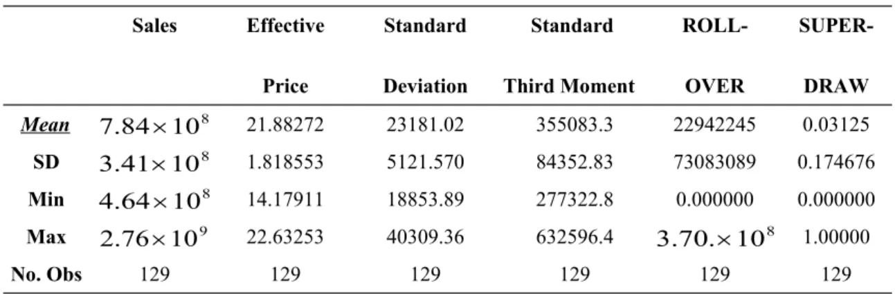
Before proceeding further, we will briefly describe our data and the basic statistics. The sample period begins from January, 2002 to April, 2003, comprising 129 observations. Summary statistics of data are given in Table 1. Sales and the effective price are measured in NT dollars. The mean of sales is around 800 million NT dollars, with a maximum of about 2.76 billion. The average effective price is 21.88272, with a minimum of 14.17911. Thus, the lotto is generally priced unfairly but the sales are consistently high. The mean of Standard Deviation and Standard
Third Moment are 23181.02 and 355083.3, respectively. But the maximum Standard Third Moment reaches 632596.4. Thus, both the risk and the skewness are very high.
Table 1 Summary Statistic Sales Effective Price Standard Deviation Standard Third Moment ROLL-OVER SUPER-DRAW Mean 7.84108 21.88272 23181.02 355083.3 22942245 0.03125 SD 3.41108 1.818553 5121.570 84352.83 73083089 0.174676 Min 4.64108 14.17911 18853.89 277322.8 0.000000 0.000000 Max 2.76109 22.63253 40309.36 632596.4 3.70.108 1.00000 No. Obs 129 129 129 129 129 129
Stage 1: ) , , (Q 1 SUPERDRAW ROLLOVER f P t Stage 2: P SUPERDRAW Q g Qt ( t1, , ˆ) where
P is the effective price and is equal to the price of ticket minus the expected value of
prize receipt (EV)5;
Pˆ is the estimated effective price; t
Q is the number of the tickets sold; Qt1 is a lagged dependent variable included
to capture persistence in sales;6
ROLLOVER represents the amount carried over (not won) from the immediately preceding draw and added to the jackpot pool in the current draw.
SUPERDRAW is a dummy variable that takes the value of one for a specific draw guaranteed by Taipei Bank to reach an announced figure.
Our model (Model II) is as follows: Stage 1: ) , , ( 1 1 Q SUPERDRAW ROLLOVER f P t
Second Moment f2(Qt1,SUPERDRAW,ROLLOVER)
5 Traditional models evaluate the effective price by unit-value ticket. Since the price of a lottery ticket
in Taiwan is always equal to 50, we do not calculate the effective price per unit-value ticket.
6 Forrest, Simmons and Chesters (2002) experimented with six lags of the dependent variables to
capture a richer pattern of habit persistence, but lags of order two and above were always jointly insignificant. Therefore we use a one-lag-variable model.
Third Moment f3(Qt1,SUPERDRAW,ROLLOVER) Stage 2: , ˆ , , (Q 1 SUPERDRAW P g Qt t eviation D dard
Stan ˆ ,StandardTˆhird Moment) eviation
D dard
Stan ˆ and StandardTˆhird Momentare already defined above.
Other notations are the same as in model I.
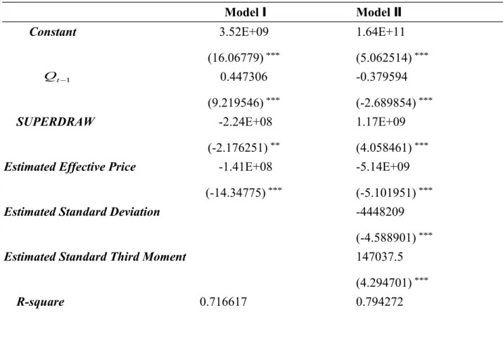
Table 2 Regression Results on the Second Stage
Model Ⅰ Model Ⅱ Constant 3.52E+09 (16.06779)*** 1.64E+11 (5.062514)*** 1 t Q 0.447306 (9.219546)*** -0.379594 (-2.689854)*** SUPERDRAW -2.24E+08 (-2.176251)** 1.17E+09 (4.058461)***
Estimated Effective Price -1.41E+08 (-14.34775)***
-5.14E+09 (-5.101951)***
Estimated Standard Deviation -4448209
(-4.588901)***
Estimated Standard Third Moment 147037.5 (4.294701)***
R-square 0.716617 0.794272
Note: Absolute values of t statistic appear in parentheses *
* Denotes significant at 5% *
*
* Denotes significant at 1%
respectively. Model Ⅰis the traditional effective price approach; Model II are our proposed alternative. We find evidences to support that the traditional effective price approach may suffer a drawback, missing important variables.
From Table 2, in Models Ⅰand II the coefficients of Estimated Effective Price are both negative, which is consistent with the traditional findings (Forrest, Simmons, and Chesters, 2002). As predicted by the theory, the estimated effective price captures the impact of lotto’s mean. Since the effective price is measured by the lotto’s nominal price minus mean and the impact of lotto’s mean on the demand should be positive, it makes perfect sense for the coefficient of the estimated effective price to be negative. Moreover, the coefficient of Estimated Effective price in Model Ⅰis much larger than that in Model II. This could suggest that the traditional model may get a biased estimator due to missing important variable, and overestimate the effect of the price.
The coefficients of Qt1 and SUPERDRAW in ModelsⅠand II are quite
different. The coefficient of Qt1 in ModelⅠ is positive and significant and was
explained in the literature by the consistency of the sales. The coefficient of Qt1 in
Model II is negative and significant. One possible explanation is “regret”. Since most bettors lose money in each game, the high sales of the previous game imply more people lost money and could have a negative impact on the sales of the next period. On the other hand, in ModelⅡ, the coefficient of SURPERDRAW is positive
and significant. One possible explanation is that the bank usually uses superdraw to simulate the demand of lotto. Our empirical results suggest this interpretation.
From Model II in Table 2, the coefficients of Estimated Standard Deviation and Estimated Standard Third Moment are significantly different from zero and are respectively negative and positive as predicted by Proposition 3.7 We also conduct
F test to examine whether both coefficients are jointly significantly different from
zero. The value of F test is 21.75 and is significant at a 1% level. The empirical results support the idea that lotto bettors could be rational players. That is, lotto bettors dislike risk but prefer standard third moment, which is consistent with the finding of Golec and Tamarkin (1998).
5. Conclusion
The paper uses the willingness-to-pay for lotto to explain why the lotto’s bettors dislike risk but prefer standard third moment of the payoff. We also propose an alternative method to examine the demand for lotto. The empirical evidence support the idea that lotto bettors could be rational. Moreover, the regression results seem to suggest that the marginal impact of the standard deviation and standard third moment are significantly different from zero. If standard deviation (respectively, standard third moment) of the lotto’s payoff increases, then the willingness-to-pay of the
individual decreases (respectively, increases).
References
Bradley, I., “The Representative Bettor, Bet Size, and Prospect Theory.” Economics
letters, 78, 2003, 409-413.
Cain, M., D. Peel, and D. Law. “Skewness as An Explanation of Gambling by Locally Risk Averse Agents.” Applied Economics Letters, 9, 2002, 1025-1028.
Cook, P. J., and C. T. Clotfelter. “The Peculiar Scale Economies of Lotto.” American
Economics Review, 83(3), 1993, 634-643.
Farrell, L., and I. Walker. “The Welfare Effects of Lotto: Evidence from the U.K.”
Journal of Public Economics, 72(1), 1999, 99-120.
Farrell, L., G. Lanot, R. Hartley, and I. Walker. “The Demand for Lotto: The Role of Conscious Selection.” Journal of Business and Economic Statistics, 18(2), 2000, 228-241.
Forrest, D., O. D. Gulley, and R. Simmons. “Testing for Rational Expectations in the U.K. National Lottery.” Applied Economics, 32(3), 2000a, 315-326.
Forrest, D., R. Simmons, N. Chesters. “Buying A Dream: Alternative Models of Demand for Lotto.” Economic Inquiry, 40(3), 2002, 485-496.
Garrent, T. A., and R. S. Sobel. “Gamblers Favor Skewness Not Risk: Further Evidence form United States’ Lottery Games.” Economic Letters, 63(1), 1999, 85-90.
Golec, J., and M. Tamarkin. “Bettors Love Skewness, Not Risk at the Horse Track.”
Journal of Political Economy, 106(1), 1998, 205-225.
Gulley, O. D., and F. A. Scott, Jr. “The Demand for Wagering on State-Operated Lottery Games.” National Tax Journal, 45(1), 1993,13-22.
Mossin, J., “Aspect of rational insurance purchasing.” Journal of Political Economy, 76, 1968, 553-568.
Pratt, H. M., “ Risk aversion in the small and in the large. “ Econometrica, 32, 1964, 217-229.
Purfield, C., and P. J. Waldron. “Gambling on Lotto Numbers: Testing for Substitutability or Complementarity Using Semi-Weekly Turnover Data.”
Oxford Bulletin of Economics and Statistics, 61(4), 1999, 527-544.
Scott, F. A. Jr., and O. D. Gulley. “Rationality and Efficiency in Lotto Markets.”
Economic Inquiry, 33(2), 1995, 175-188.
359-392.
Woodland, B. M., and L. M. Woodland. “Expected Utility, Skewness, and The Baseball Betting Market.” Applied Economics, 31, 1999, 337-345.