行政院國家科學委員會
獎勵人文與社會科學領域博士候選人撰寫博士論文
成果報告
應用增長層級式自我組織映射網路於財務舞弊偵測之研究
核 定 編 號 : NSC 100-2420-H-004-040-DR 獎 勵 期 間 : 100 年 08 月 01 日至 101 年 07 月 31 日 執 行 單 位 : 國立政治大學資訊管理研究所 指 導 教 授 : 蔡瑞煌 博 士 生 : 黃馨瑩 公 開 資 訊 : 本計畫涉及專利或其他智慧財產權,2 年後可公開查詢中 華 民 國 101 年 09 月 08 日
博士學位論文
指導教授:蔡瑞煌博士
國立政治大學資訊管理研究所
適 用 於 財 務 舞 弊 偵 測 之 決 策 支 援 系 統 的 對 偶
方 法
A Dual Approach for Decision Support in Financial
Fraud Detection
研究生:黃馨瑩
Content
Abstract ... 1
1. Introduction ... 5
2. Literature review ... 9
2.1 DSS... 9
2.2 Clustering methods and the GHSOM ... 10
2.2.1 Clustering methods and the SOM ... 10
2.2.2 GHSOM ... 14
2.3 PCA ... 17
2.4 FFR ... 21
2.5 Summary ... 27
3. The proposed dual approach ... 29
3.1 Training phase ... 30 3.1.1 Sampling module ... 31 3.1.2 Variable-selecting module ... 31 3.1.3 Clustering module... 32 3.2 Modeling phase ... 32 3.2.1 Statistic-gathering module ... 34 3.2.2 Rule-forming module ... 35 3.2.3 Feature-extracting module ... 37 3.2.4 Pattern-extracting module ... 39 3.3 Analyzing phase ... 39 3.3.1 Group-finding module ... 40 3.3.2 Classifying module ... 40
3.4 Decision support phase... 41
3.4.1 Feature-retrieving module ... 41
3.4.2 Decision-supporting module... 42
4. The FFR experiment and results ... 45
4.1 Training phase – sampling module ... 45
4.2 Training phase – variable-selecting module ... 49
4.4 Modeling phase – statistic-gathering, rule-forming module ... 64
4.5 Modeling phase – feature-extracting module ... 69
4.6 Modeling phase – pattern-extracting module ... 76
4.7 Analyzing phase – group-finding, classifying module ... 80
4.8 Decision support phase – feature-retrieving module ... 81
4.8.1 Retrieve from pattern-extracting module ... 81
4.8.2 Retrieve from feature-extracting module ... 83
4.9 Analyzing phase – decision-supporting module ... 84
5. Methods comparison ... 87 5.1 SVM ... 87 5.2 SOM+LDA ... 88 5.3 GHSOM+LDA ... 89 5.4 SOM ... 91 5.5 BPNN ... 92 5.6 DT... 94
5.7 Discussion of the experimental results ... 97
6. Discussions and implications ... 98
6.1 The decision support in FFD ... 99
6.2 The research implications ... 100
6.3 The FFR managerial implications ... 102
7. Conclusion ... 104
Reference ... 107
List of Tables
Table 1. Research methodology and findings in nature-related FFR studies. ... 23
Table 2. Research methodology and findings in FFR empirical studies. ... 25
Table 3. The training phase. ... 31
Table 4. The modeling phase. ... 32
Table 5. The analyzing phase. ... 40
Table 6. The decision support phase. ... 41
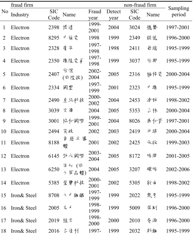
Table 7. The list of fraud and non-fraud firms in training samples. ... 46
Table 8. Variable definition and measurement. ... 58
Table 9. Empirical results of discriminant analysis. ... 61
Table 10. The GHSOM parameter setting trials. ... 62
Table 11. The leaf node matching from NFT to FT. ... 64
Table 12. The result of w1 and w2 of the non-fraud-central rule. ... 66
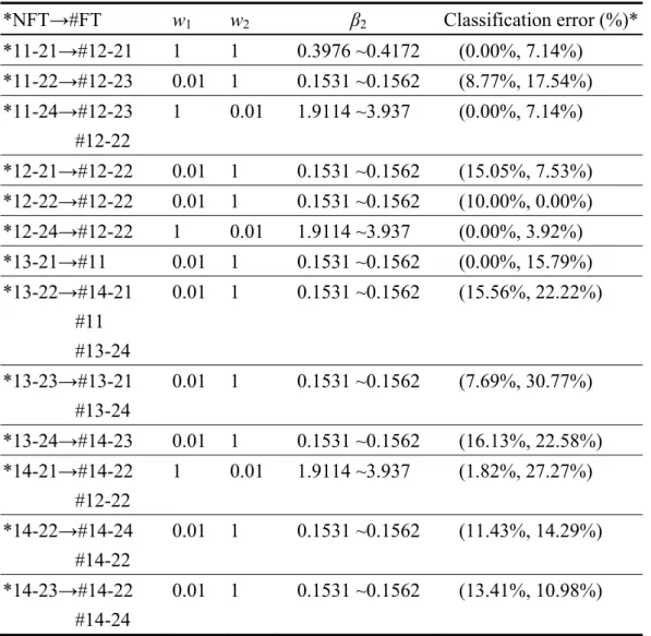
Table 13. The leaf node matching from FT to NFT. ... 67
Table 14. The result of w1 and w2 of the fraud-central rule. ... 68
Table 15. The estimated eigenvalues of eight factors regarding all FT leaf nodes. ... 69
Table 16. The factor loadings of all FT leaf nodes. ... 73
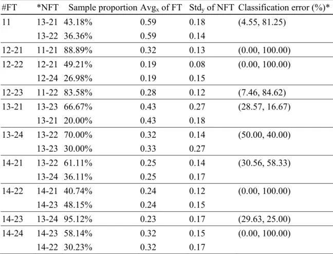
Table 17. Common FFR fraud categories within #11 and #14-24. ... 77
Table 18. Summary of the common FFR fraud categories. ... 79
Table 19. The list of fraud and non-fraud firms in testing samples. ... 80
Table 20. The classification result. ... 81
Table 21. The overall FFR fraud categories identification performance. ... 82
Table 22. The principle components retrieved by the feature-retrieving module for the testing samples within #11 and #14-24. ... 83
Table 23. The results of decision-supporting module for any investigated sample identified fraud. ... 85
Table 24. The habitual working procedure of the SOM+LDA. ... 89
Table 25. The habitual working procedure of the GHSOM+LDA. ... 90
Table 26. The habitual working procedure of the SOM. ... 91
Table 27. The weights of BPNN. ... 93
Table 29. The experimental results of our dual approach, the SVM, SOM+LDA,
GHSOM+LDA, SOM, BPNN and DT methods. ... 96
Table A1. Common FFR fraud categories within all leaf nodes of FT. ... 116
Table A2. Common FFR fraud categories of the testing samples. ... 120
List of Figures
Figure 1. The self organizing map structure ... 12
Figure 2. The GHSOM structure. ... 15
Figure 3. Horizontal growth of individual SOM. ... 16
Figure 4. The main steps of the PCA. ... 20
Figure 5. System architecture of the proposed dual approach. ... 30
Figure 6. The classification concept of the proposed dual approach. ... 44
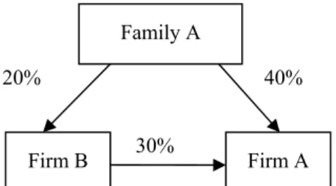
Figure 7. An example of control right and cash flow right. ... 56
Figure 8. The obtained FT and NFT. ... 63
Figure 9. The leaf node matching from NFT to FT. ... 65
Figure 10. The leaf node matching from FT to NFT. ... 67
Figure 11. The map size of the SOM in the SOM+LDA method. ... 89
Figure 12. The obtained GHSOM tree of the GHOM+LDA method. ... 90
Figure 13. The map size of the SOM with FFR proportions. ... 92
Figure 14. The BPNN structure. ... 93
Figure 15. The obtained DT structure. ... 95
Abstract
The Growing Hierarchical Self-Organizing Map (GHSOM) is extended from the Self-Organizing Map (SOM). The GHSOM’s unsupervised learning nature such as the adaptive group size as well as the hierarchy structure renders its availability to discover the statistical salient features from the clustered groups, and could be used to set up a classifier for distinguishing abnormal data from regular ones based on spatial relationships between them.
Therefore, this study utilizes the advantage of the GHSOM and pioneers a novel dual approach (i.e., a proposal of a DSS architecture) with two GHSOMs, which starts from identifying the counterparts within the clustered groups. Then, the classification rules are formed based on a certain spatial hypothesis, and a feature extraction mechanism is applied to extract features from the fraud clustered groups. The dominant classification rule is adapted to identify suspected samples, and the results of feature extraction mechanism are used to pinpoint their relevant input variables and potential fraud activities for further decision aid.
Specifically, for the financial fraud detection (FFD) domain, a non-fraud (fraud) GHSOM tree is constructed via clustering the non-fraud (fraud) samples, and a non-fraud-central (fraud-central) rule is then tuned via inputting all the training samples to determine the optimal discrimination boundary within each leaf node of the non-fraud (fraud) GHSOM tree. The optimization renders an adjustable and effective rule for classifying fraud and non-fraud samples. Following the implementation of the DSS architecture based on the proposed dual approach, the decision makers can objectively set their weightings of type I and type II errors. The classification rule that dominates another is adopted for analyzing samples. The dominance of the non-fraud-central rule leads to an implication that most of fraud samples cluster around the non-fraud counterpart, meanwhile the dominance of fraud-central rule leads to an implication that most of non-fraud samples cluster around the fraud counterpart.
Besides, a feature extraction mechanism is developed to uncover the regularity of input variables and fraud categories based on the training samples of each leaf node of a fraud GHSOM tree. The feature extraction mechanism involves extracting the variable features and fraud patterns to explore the characteristics of fraud samples within the same leaf node. Thus can help decision makers such as the capital providers
evaluate the integrity of the investigated samples, and facilitate further analysis to reach prudent credit decisions.
The experimental results of detecting fraudulent financial reporting (FFR), a sub-field of FFD, confirm the spatial relationship among fraud and non-fraud samples. The outcomes given by the implemented DSS architecture based on the proposed dual approach have better classification performance than the SVM, SOM+LDA, GHSOM+LDA, SOM, BPNN and DT methods, and therefore show its applicability to evaluate the reliability of the financial numbers based decisions. Besides, following the SOM theories, the extracted relevant input variables and the fraud categories from the GHSOM are applicable to all samples classified into the same leaf nodes. This principle makes that the extracted pre-warning signal can be applied to assess the reliability of the investigated samples and to form a knowledge base for further analysis to reach a prudent decision. The DSS architecture based on the proposed dual approach could be applied to other FFD scenarios that rely on financial numbers as a basis for decision making.
Keywords: Growing Hierarchical Self-Organizing Map; Unsupervised Neural Networks; Classification; Financial Fraud Detection; Fraudulent Financial Reporting.
摘 要
增長層級式自我組織映射網路(GHSOM)屬於一種非監督式類神經網路,為自 我組織映射網路(SOM)的延伸,擅長於對樣本分群,以輔助分析樣本族群裡的共 同特徵,並且可以透過族群間存在的空間關係假設來建立分類器,進而辨別出異 常的資料。 因此本研究提出一個創新的對偶方法(即為一個建立決策支援系統架構的方 法)分別對舞弊與非舞弊樣本分群,首先兩類別之群組會被配對,即辨識某一特定 無弊群體的非舞弊群體對照組,針對這些配對族群,套用基於不同空間假設所設 立的分類規則以檢測舞弊與非舞弊群體中是否有存在某種程度的空間關係,此外 並對於舞弊樣本的分群結果加入特徵萃取機制。分類績效最好的分類規則會被用 來偵測受測樣本是否有舞弊的嫌疑,萃取機制的結果則會用來標示有舞弊嫌疑之 受測樣本的舞弊行為特徵以及相關的輸入變數,以做為後續的決策輔助。 更明確地說,本研究分別透過非舞弊樣本與舞弊樣本建立一個非舞弊GHSOM 樹以及舞弊GHSOM 樹,且針對每一對 GHSOM 群組建立分類規則,其相應的非 舞弊/舞弊為中心規則會適應性地依循決策者的風險偏好最佳化調整規則界線,整 體而言較優的規則會被決定為分類規則。非舞弊為中心的規則象徵絕大多數的舞 弊樣本傾向分布於非舞弊樣本的周圍,而舞弊為中心的規則象徵絕大多數的非舞 弊樣本傾向分布於舞弊樣本的周圍。 此外本研究加入了一個特徵萃取機制來發掘舞弊樣本分群結果中各群組之樣 本資料的共同特質,其包含輸入變數的特徵以及舞弊行為模式,這些資訊將能輔 助決策者(如資本提供者)評估受測樣本的誠實性,輔助決策者從分析結果裡做出 更進一步的分析來達到審慎的信用決策。 本研究將所提出的方法套用至財報舞弊領域(屬於財務舞弊偵測的子領域)進 行實證,實驗結果證實樣本之間存在特定的空間關係,且相較於其他方法如 SVM、SOM+LDA 和 GHSOM+LDA 皆具有更佳的分類績效。因此顯示本研究所 提出的機制可輔助驗證財務相關數據的可靠性。此外,根據 SOM 的特質,即任 何受測樣本歸類到某特定族群時,該族群訓練樣本的舞弊行為特徵將可以代表此 受測樣本的特徵推論。這樣的原則可以用來協助判斷受測樣本的可靠性,並可供 持續累積成一個舞弊知識庫,做為進一步分析以及制定相關信用決策的參考。本 研究所提出之基於對偶方法的決策支援系統架構可以被套用到其他使用財務數據 為資料來源的財務舞弊偵測情境中,作為輔助決策的基礎。關鍵詞: 增長層級式自我組織映射網路;非監督式類神經網路;分類;財務舞弊 偵測;財務報表舞弊
1. Introduction
This study proposes a dual approach as a Decision Support System (DSS) architecture based on the Growing Hierarchical Self-Organizing Map (GHSOM) (Dittenbach et al., 2000; Dittenbach et al., 2002; Rauber et al., 2002), a type of unsupervised artificial neural networks (ANN), for the decision support in financial fraud detection (FFD). FFD involves distinguishing fraudulent financial data from authentic data, disclosing fraudulent behavior or activities, and enabling decision makers to develop appropriate strategies to decrease the impact of fraud (Lu and Wang, 2010). The decision for FFD can be aided by statistical methods such as the logistic regression, as well as data mining tools such as the ANN, in which the ANN has been widely used and plays an important role in FFD (Lu and Wang, 2010). Among the ANN applications in FFD, the Self-Organizing Map (SOM) (Kohonen, 1982) has been adopted in diagnosing bankruptcy (Carlos, 1996). The major advantage of the SOM is its great visualization capability of topological relationship among the high-dimensional inputs in the low-dimensional view. Other advantages are adaptive (i.e., the clustering can be redone if new training samples are set) and robust (i.e., the pattern recognition ability). There are numerous applications involving the SOM and the most widespread use is the identification and visualization of natural groupings in the sample data sets. However, the weaknesses of the SOM include its predefined and fixed topology size and its inability to provide the hierarchical relations among samples (Dittenbach et al., 2000).
An improvement of the SOM has been done by Dittenbach, Merkl and Rauber (2000). They developed the GHSOM which addresses the issue of fixed network architecture of the SOM through developing a multilayer hierarchical network structure. The flexible and hierarchical feature of the GHSOM generates delicate clustered subgroups with heterogeneous features, and makes it a powerful and versatile data mining tool. The GHSOM has been used in many fields such as the image recognition, web mining, text mining, and data mining (Dittenbach et al., 2000; Schweighofer et al., 2001; Dittenbach et al., 2002; Rauber et al., 2002; Shih et al., 2008; Zhang and Dai, 2009; Tsaih et al., 2009). It is worth of knowing that the GHSOM can be a useful clustering tool to do the pre-processing of feature extraction for a certain application field.
In general, the GHSOM mainly takes the task of clustering and then visualizing the clustering results. To accomplish other purposes such as prediction or classification, the neural networks must be complemented with a statistical study of the available information (Serrano, 1996). However, this study finds that the development of the GHSOM into a classification model has been limited studied (Hsu et al., 2009; Lu and Wang, 2010; Guo et al., 2011). Besides, other than the hierarchical feature, the GHSOM studies have rarely provided the topological insight into high-dimensional inputs.
To better utilize the advantage of the GHSOM for the purpose of classification and feature extraction in helping FFD, this study pioneers a DSS architecture based on the proposed dual approach which helps extract the nature of the distinctive characteristics among different clustered groups generated by the GHSOM. This study develops an innovative way of observing the clustered data to form the optimal classification rule, and revealing more information regarding the relevant input variables and the potential fraud categories for the suspected samples as the knowledge base for facilitating FFD decision making.
This study examines the following topological relationships regarding high-dimensional inputs, of which there are two types: fraud and non-fraud, and matches the fraud counterpart of each non-fraud subgroup and vice versa. This study assumes that there is a certain spatial relationship among fraud and non-fraud samples. The spatial hypothesis: The spatial distributions of fraud samples and their non-fraud counterparts are identical, and the spatial distributions of most fraud samples and their non-fraud counterparts are the same. Within each pair of clusters, either the fraud samples cluster around their non-fraud counterparts, or the non-fraud samples cluster around their fraud counterparts. If such a spatial relationship among fraud and non-fraud samples does exist, the associated classification rule can be set up to identify the fraud samples based on the correspondence of the fraud samples and their non-fraud counterparts and vice versa. Moreover, the proposed dual approach is data-driven. That is, the corresponding system modeling is performed via directly using the sampled data. Thus, different sampled data input to the proposed DSS architecture may result in distinctive DSSs. To practically utilize such a spatial relationship for identifying fraud cases and examine the applicability of the proposed
DSS architecture based on the dual approach, this study sets up the fraudulent financial reporting (FFR) experiment, a sub-field of FFD.
Specifically, the proposed DSS architecture contains four phases. In the training phase, the sampling and variable selection are done first, and then it adopts the hierarchal-topology mapping advantage of the GHSOM to build up two GHSOMs (named non-fraud tree, NFT, and fraud tree, FT) from two classes of training samples collected from the financial statements.
In the modeling phase, following the majority principle, the corresponsive FT leaf node for each NFT leaf node are identified using all (fraud and non-fraud) training samples. Then, each training sample is classified into these two GHSOMs to develop the discrimination boundaries according to the candidate classification rules. The candidate classification rules in this study involve a non-fraud-central rule and a fraud-central rule, which are tuned via inputting the clustered training samples to determine the optimal discrimination boundary within each leaf node of the FT and NFT. For the candidate classification rules, a decision maker can set up his/her preference for the weights of classification error (type I and type II error) that makes the developed classification rule more acceptable and domain specific. The dominant classification rule with the best classification performance is applied in the analyzing phase. Besides, this study involves a feature extraction mechanism with two modules, feature-extracting module and pattern-extracting module, in the modeling phase that focus on discovering the common features and patterns in each FT leaf node. For the features regarding the input variables, the principal component analysis (PCA) is applied to provide the associated principal components. For the patterns such as the FFR fraud categories, the corresponding verdict contents of the fraud samples are investigated to determine the associated FFR fraud categories.
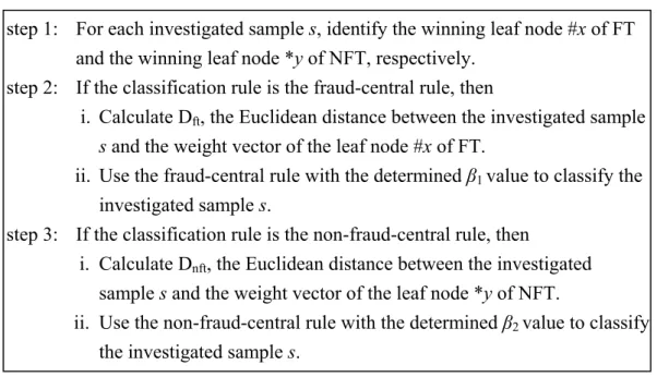
In the analyzing phase, each investigated sample is classified into the winning leaf nodes of FT and NFT, and applies the dominant classification rule to determine whether this sample is fraud or not. In the decision support phase, for an investigated sample, the result of the analyzing phase is used to help the decision makers speculate its FFR potentiality and. If it is identified as fraud, the associated potential FFR behaviors will be retrieved. The released information of the implemented DSS architecture based on the proposed dual approach can help decision makers better identify FFR and interpret the distinctive FFR behaviors among the clustered groups,
comprehend the difference between fraud and non-fraud samples, and finally facilitate the real-world decision making.
In sum, the implementation of the DSS architecture based on the proposed dual approach can be leveraged both to justify the spatial hypothesis, and when the spatial hypothesis holds, to disclose the information that better supports FFD. The proposed DSS architecture based on the dual approach is expected to be potentially applicable to other similar scenarios, and is able to be implemented as a DSS that helps detect suspicious samples and at the same time provide their possible fraud categories beforehand.
There are four objectives of this study:
(1) Develop a DSS architecture based on the proposed dual approach that (a) adopt the GHSOM to separately cluster fraud training samples and non-fraud training samples; (b) set up the discriminant boundaries for each pair of leaf nodes following the candidate classification rules based on the proposed spatial hypotheses; (c) use the determined classification rule to classify unknown samples; (d) observe whether spatial hypothesis holds and (d) illustrate the embedded information from the evaluation results including the extracted features and fraud patterns from the FT leaf nodes.
(2) Justify whether the implemented dual approach is capable of helping distinguish fraud and non-fraud samples.
(3) Compare the outcomes of our classification with other supervised or unsupervised learning methods.
(4) Provide implications regarding FFD decision support and research implications. The rest of this dissertation is organized as follows. Chapter Two presents the literature reviews of the DSS, clustering methods, the GHSOM, PCA and FFR. Chapter Three explains the design of the proposed dual approach in details. Chapter Four demonstrates the experimental results. Chapter Five provides the comparison against other methods and the discussion of experiment of results. The implications are shown in Chapter Six. Chapter Seven gives the final conclusion and future works.
2. Literature review
In this section, we briefly review the DSS, clustering methods, GHSOM, PCA and FFR as the background knowledge including the applications of the GHSOM and the FFR detection issue.
2.1 DSS
Basically, the efforts in supporting the whole decision-making process focused in the development of computer information systems providing the support needed. The concept of the DSS was introduced, from a theoretical point of view, in the last 1960s. Klein and Methlie (1995) define a DDS as a computer information system that provides information in a specific problem domain using analytical decision models as well as techniques and access to database, in order to support a decision maker in taking decision effectively in complex and ill-structured problems. The contribution of DSS technology can be summarized as follows (Turban, 1993):
z The DSSs provide the necessary means for dealing with semi-structured and unstructured problems of high complexity, such as many problems from the field of financial management.
z The support provided by the DSSs may respond to the needs and the cognitive style of different decision makers, combining the preferences and the judgment of the every individual decision maker with the information derived by analytical decision models.
z The time and the cost of the whole decision process are significantly reduced. z The support that is provided by the DSSs responds to the needs of various
managerial levels, ranging from top managers and executives down to staff managers.
The DSSs help the decision maker to gain experience in data collection, as well as in the implementation of several scientific decision models, and they also incorporate the preferences and decision policy of the decision maker in the decision-making process. (Zopounidis et al., 1997)
There are various researches that have developed the DSSs for many application areas, for example, HR planning and decisions (Mohanty and Deshmukh, 1997),
financial management (Matsatsinis et al., 1997), marketing (Li, 2000), etc. Pinson (1992) developed the CREDEX system, which demonstrated the feasibility of a multi-expert approach driven by a meta-model in the assessment of credit risk. The system, using quantitative (economic and financial) and qualitative (social) data concerning the examined company and its business sector, as well as the bank’s lending policy, provides a diagnosis of the company's function (commercial, financial, managerial and industrial) in terms of weaknesses and strengths. Zopounidis et al. (1997) developed a knowledge-based decision support system for financial management that integrates the DSS technologies to tackle past and current frequently occurring problems. Wen et al. (2005) proposed a decision support system based on an integrated knowledge base for acquisitions and mergers. It not only provided information concerning merger processes, major problems likely to occur in merger situations, and regulations practically or procedurally, but also gave rational suggestions in compliance with the appropriate regulations. It also suggested to the user how to deal with an uncertain growth rate and current evaluations. Wen et al. (2008) presented a mobile knowledge management decision support system using multi-agent technology for automatically providing efficient solutions for decision making and managing an electronic business. Nguyen et al. (2008) proposed an early warning system (EWS) that identifies potential bank failures or high-risk banks through the traits of financial distress which is able to identify the inherent traits of financial distress based on financial covariates (features) derived from publicly available financial statements.
In sum, many methodologies have been used and embedded with the existing framework of the DSS that could considerably increase the effectiveness of the provided decision support.
2.2 Clustering methods and the GHSOM
2.2.1 Clustering methods and the SOM
Clustering is an unsupervised classification of patterns into groups based on similarity. The main goal of clustering is to partition data patterns into several homogeneous groups that minimizes within-group variation and maximizes between
group variations. Each group is represented by the centroid of the patterns that belongs to the group. There are many important applications of clustering such as image segmentation (Jain et al., 1999), object recognition, information retrieval (Rasmussen, 1992), and so on. Clustering is the process of grouping the similarity data together such that data is high similarity within cluster but are dissimilarity between clusters. Clustering is the basis of many areas including data mining, statistical, biology, machine learning, etc. Clustering methods are used for data exploration and to provide class prototypes for use in the supervised classifiers. Among many clustering tools, the SOM is an unsupervised learning ANN and it appears to be an effective method for feature extraction and classification. Therefore, this study gives the following introduction and some literature reviews.
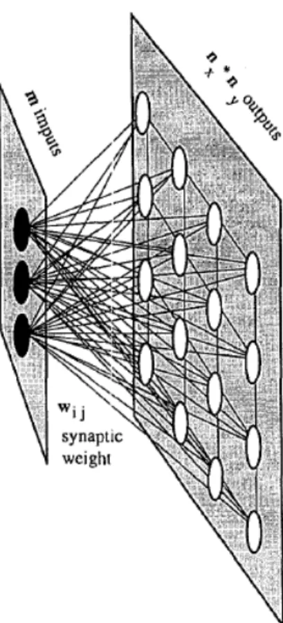
The Self-Organizing Map (SOM) is developed by Kohonen (1982), also known as the Kohonen Maps. It has demonstrated its efficiency in real domains, including clustering, the recognition of patterns, the reduction of dimensions, and the extraction of features. It maps high-dimensional input data onto a low dimensional space while preserving the topological relationships between the input data. SOM is made up two neural layers. The input layer has as many neurons as it has variables, and its function is merely to capture the information. Let m be the number of neurons in the input layer; and let nx * ny the number of neurons in the output layer which are arranged in a
rectangular pattern with x rows and y columns, which is called the map. Each neuron in the input layer is connected to each neuron in the output layer. Thus, each neuron in the output layer connections to the input layer. Each one of these connections has a synaptic weight associated with it. Let wij the weight associated with the connection
between input neuron i and output neuron j. Figure 1 gives a visual representation of this neural arrangement.
Figure 1. The self organizing map structure
Note: This SOM with m neurons in the input layer and nx * ny neurons in the output
layer. Each neuron in the output layer has m connections wij (synaptic weights) to the
input layer (Carlos, 1996).
SOM tries to project the multidimensional input space, which in our case could be financial information, into the output space in such a way that the input patterns whose variables present similar values appear close to one another on the map which is created. Each neuron learns to recognize a specific type of input pattern. Neurons which are close on the map will recognize similar input patterns whose images therefore, will appear close to one another on the created map. In this way, the essential topology of the input space is preserved in the output space. In order to achieve this, the SOM uses a competitive algorithm known as “winner takes all”.
Initially, the wij are given random values. These values will be corrected as the
algorithm progress. Training proceeds by presenting the input layer with financial ratios, one sample at a time. Let rik be the value of ratio i for firm k. This ratio will be
read by neuron i. The algorithm takes each neuron in the output layer at a time and computes the Euclidean distance as the similarity measure.
∑
− = i ijk ik w r k j d( , ) ( )2 (1)The output neuron for which d(j, k) (defined in Equation (1)) is the smallest, and is the “winner neuron”. Let such neuron be k*. The algorithm now proceeds to change the synaptic weights wij in such a way that the distance d(j, k*) is reduced. A correction
takes place, which depends on the number of iterations already performed and on the absolute value of the difference between rij and wijk. But other synaptic weights are also
adjusted in function to how near they are to the winning neuron k* and the number of iterations that have already taken place.
The procedure is repeated until complete training stops. Once the training is complete, the weights are fixed and the network is ready to be used. When a new pattern is presented, each neuron computes in parallel the distance between the input vector and the weight vector that it stores, and a competition starts that is won by the neuron whose weights are more similar to the input vector. Alternatively, we can consider the activity of the neurons on the map (inverse to the distance) as the output. The region where the maximum activity takes place indicates the class that the present input vector belongs to. If a new pattern is presented to the input layer and no neuron is stimulated by its presence the activity will be minimal, and this means that the pattern is not recognized. (Kohonen, 1989).
Thousands of the SOM applications are found among various disciplines (Serran, 1996; Richardson et al., 2003; Risien et al., 2004; Liu et al., 2006). It is widely used in application to the analysis of financial information (Serran, 1996). Eklund (2002) indicated that the SOM can be a feasible tool for classification of large amounts of financial data. The SOM has established its position as a widely applied tool in data-analysis and visualization of high-dimensional data. Within other statistical methods the SOM has no close counterpart, and thus it provides a complementary view to the data. The SOM is a widely used method in classification or clustering problem, because it provides some notable advantages over the alternatives (Khan et al., 2009).
There are various studies that used the SOM for a given clustering problem. Mangiameli, Chen, and West (1996) compared the performance of the SOM and seven hierarchical clustering methods for 252 data sets with various levels of imperfections that include data dispersion, outliers, irrelevant variables and non-uniform cluster densities. In conclusion, they demonstrated that the SOM is superior to the hierarchical
clustering methods. Granzow et al. (2001) investigated five clustering techniques: K-means, SOM, growing cell structure networks, fuzzy C-means (FCM) algorithm and fuzzy SOM. At the end of the analysis, they concluded that fuzzy SOM approach is the most suitable method in partitioning the data set. Shin and Sohn (2004) used K-means, SOM and FCM in order to segment stock trading customers and inferred that FCM cluster analysis is the most robust approach for segmentation of customers. Martín-Guerrero et al. (2006) compared the performance of K-means, FCM, and a set of hierarchical algorithms, Gaussian mixtures trained by the expectation–maximization algorithm, and the SOM in order to determine the most suitable algorithm in classification of artificial data sets produced for web portals. Finally, they concluded that the SOM outperforms the other clustering methods. Budayan et al. (2009) presented the strategic group analysis of Turkish contractors to compare the performances of traditional cluster analysis techniques, SOM and FCM for strategic grouping. It is concluded that the SOM and FCM can reveal the typology of the strategic groups better than traditional cluster analysis and they are more likely to provide useful information about the real strategic group structure.
The difference findings of these studies can be explained by the argument that the suitability of clustering methods to a given problem changes with the structure of the data set and purpose of the study. It is concluded that the aim of a study using clustering method is not to find out the best clustering method for all data sets and fields of application, but instead it is to demonstrate superior features of different clustering techniques for a particular problem domain, for example the FFD.
2.2.2 GHSOM
The SOM has shown to be a stable neural network model of high-dimensional data analysis. However, its capability is limited by some limitations when using the SOM. The first drawback is its static network architecture. The number and arrangement of nodes has to be pre-defined even without a priori knowledge of the data. Second, the SOM model has limited capabilities for the representation of hierarchical relations of the data. To overcome the inherent deficiencies of the SOM, Dittenbach, Merkl, and Rauber (2000) developed GHSOM to provide a SOM hierarchy automatically.
As shown in Figure 2, the GHSOM contains a number of SOMs in each layer. The size of these SOMs and the depth of the hierarchy are determined during its learning process according to the requirements of the input data.
Figure 2. The GHSOM structure.
The training process of the GHSOM consists of the following four phases (Dittenbach et al., 2000):
z Initialize the layer 0: The layer 0 includes single node whose weight vector is initialized as the expected value of all input data. Then, the mean quantization error of layer 0 (MQE0) is calculated. The MQE of a node denotes the mean
quantization error that sums up the deviation between the weight vector of the node and every input data mapped to the node.
z Train each individual SOM: Within the training process of an individual SOM, the input data is imported one by one. The distances between the imported input data and the weight vector of all nodes are calculated. The node with the shortest distance is selected as the winner. Under the competitive learning principle, only the winner and its neighborhood nodes are qualified to adjust their weight vectors. Repeat the competition and the training until the learning rate decreases to a certain value.
z Grow horizontally each individual SOM: Each individual SOM will grow until the mean value of the MQEs for all of the nodes on the SOM (MQEm) is
smaller than the MQE of the parent node (MQEp) multiplied by τ1 as stated in
owns the largest MQE and then, as shown in Figure 3, insert one row or one column of new nodes between the error node and its dissimilar neighbor.
MQEm < τ1 × MQEp (2)
Figure 3. Horizontal growth of individual SOM.
Note: The notation x indicates the error node and y indicates the x’s dissimilar neighbor.
z Expand or terminate the hierarchical structure: After the horizontal growth phase of individual SOM, each MQEi is compared with the value of MQE0
multiplied by τ2. The node with an MQEi greater than τ2 × MQE0 will develop
a next layer of SOM. In this way, the hierarchy grows until all of the leaf nodes satisfy the stopping criterion stated in Equation (3). The leaf nodes means the node does not own a next layer of SOM.
MQEi < τ2 × MQE0 (3)
Several researches have applied the GHSOM to deal with text mining, image recognition and web mining problem. For example, Schweighofer et al. (2001) have show the feasibility of using the GHSOM and LabelSOM techniques in legal research by tests with text corpora in European case law. Shih et al. (2008) used the GHSOM algorithm to present a content-based and easy-to-use map hierarchy for Chinese legal documents in the securities and futures markets in the Chinese language. Antonio et al. (2008) used the GHSOM to analyze a citizen web portal, and provided a new visualization of the patterns in the hierarchical structure. The results have shown that the GHSOM is a powerful and versatile tool to extract relevant and straightforward knowledge from the vast amount of information involved in a real citizen web portal. Lu and Wang (2010) applied the GHSOM with support vector regression model to
product demand forecasting. The experimental results showed that the GHSOM can be used to combine with other machine learning or data mining techniques in order to improve the performance and obtain inspirable results.
Not many studies have applied the GHSOM in the purpose of forecasting until recent years. For instance, the two-stage architecture is employed by Hsu et al. (2009) which applied GHSOM and SVM to better predict financial indices. They suggested that the two-stage architecture can have smaller deviations between predicted and actual values than the single SVM model. Lu and Wang (2010) applied the GHSOM with support vector regression model to product demand forecasting. Guo et al. (2011) applied the GHSOM in case base reasoning system in design domain and found that new case is guided into corresponding sub-case base through the GHSOM, which makes the case retrieval more efficient and accurate. In sum, the GHSOM has been used in combining with other machine learning or data mining techniques to improve the model performance, and to provide valuable information for decision aid.
2.3 PCA
Feature extraction is an essential pre-processing step to pattern recognition and machine learning problems. It is often decomposed into feature construction and feature selection. Feature selection approaches try to find a subset of the original variables, which are generally performed before or after model training. In some cases, data analysis such as regression or classification can be done in the reduced space more accurately than in the original space. Feature selection can be done by using different methods, such as the PCA, Factor Analysis (FA), stepwise regression, and discriminant analysis (Tsai, 2009). In terms of the usage of dependent variable, these methods could be divided into supervised and unsupervised categories. Supervised feature selection techniques usually relate to the discriminant analysis technique (Fukunaga, 1990) which uses the within and between-class scatter matrices. Unsupervised linear feature selection techniques more or less all rely on the PCA (Pearson, 1901), which rotates the original feature space and projects the feature vectors onto a limited amount of axes (Turk and Pentland, 1991; Oja, 1992).
The PCA was invented by Pearson (1901). The central idea of PCA is to reduce the dimensionality of a data set consisting of a large number of interrelated variables, while retaining as much as possible of the variation present in the data set. This is achieved by transforming to a new set of uncorrelated principal components (PCs), which are ordered so that the first few retain most of the variation present in all of the original variables (Jolliffe, 2002).
The PCA can be done by eigenvalue decomposition of a data covariance matrix or singular value decomposition of a data matrix, usually after mean centering the data for each attribute. The results of a PCA are usually discussed in terms of component scores (the transformed variable values corresponding to a particular case in the data) and loadings (the variance each original variable would have if the data are projected onto a given PCA axis) (Shaw, 2003).
The PCA is mathematically defined as an orthogonal linear transformation that transforms the data to a new coordinate system such that the greatest variance by any projection of the data comes to lie on the first coordinate (called the first principal component), the second greatest variance on the second coordinate, and so on (Jolliffe, 2002).
Define a data matrix, XT, with zero empirical mean (the empirical mean of the distribution has been subtracted from the data set), where each of the n rows represents a different repetition of the experiment, and each of the m columns gives a particular kind of datum (say, the results from a particular probe). (Note that what we are calling XT is often alternatively denoted as X itself.) The PCA transformation is then given by below Equation (4):
T T
T X W VΣ
Y = = (4)
where the matrices W, Σ, and V are given by a singular value decomposition (SVD) of X as W Σ VT. (V is not uniquely defined in the usual case when m < n−1, but Y will
usually still be uniquely defined.) Σ is an m-by-n diagonal matrix with nonnegative real numbers on the diagonal. Since W (by definition of the SVD of a real matrix) is an orthogonal matrix, each row of YT is simply a rotation of the corresponding row of XT. The first column of YT is made up of the "scores" of the cases with respect to the
principal component, and the next column has the scores with respect to the second principal component. If we want a reduced-dimensionality representation, we can
project X down into the reduced space defined by only the first L singular vectors, WL defined in Equation (5): T L T L X V W Y= =ΣL (5)
The matrix W of singular vectors of X is equivalently the matrix W of eigenvectors of the matrix of observed covariance C = X XT defined in Equation (6),
T T
T W W
XX = ΣΣ (6)
Given a set of points in Euclidean space, the first principal component corresponds to a line that passes through the multidimensional mean and minimizes the sum of squares of the distances of the points from the line. The second principal component corresponds to the same concept after all correlation with the first principal component has been subtracted out from the points. The singular values (in Σ) are the square roots of the eigenvalues of the matrix XXT. Each eigenvalue is proportional to the portion of the "variance" (more correctly of the sum of the squared distances of the points from their multidimensional mean) that is correlated with each eigenvector. The sum of all the eigenvalues is equal to the sum of the squared distances of the points from their multidimensional mean. The PCA essentially rotates the set of points around their mean in order to align with the principal components. This moves as much of the variance as possible (using an orthogonal transformation) into the first few dimensions. The values in the remaining dimensions, therefore, tend to be small and may be dropped with minimal loss of information. The PCA is often used in this manner for dimensionality reduction. (Jolliffe, 2002)
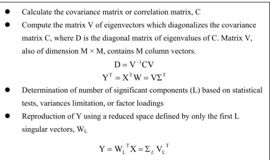
The result of PCA is a linear transformation that transforms the data to a new coordinate system such that the new set of variables, also called the principal components. This linear function of the original variables are uncorrelated and the greatest variance by any projection of the data comes to lie on the first coordinate, the second greatest variance on the second coordinate, and so on. The main steps of the PCA are summarized in Figure 4.
Figure 4. The main steps of the PCA.
In short, the PCA is achieved by transforming to a new set of variables, as the principal components, which are uncorrelated and ordered so that the first few retain most of the variation present in the entire original variables (Jolliffe, 1986). By using a few components, each sample can be represented by relatively few numbers instead of by values for thousands of variables. Samples can then be plotted, making it possible to visually assess similarities and differences between samples and determine whether samples can be grouped. (Ringnér, 2008)
Many studies have used the PCA for feature selection or dimensional reduction in financial studies. For example, Canbas et al. (2005) used the PCA to construct an integrated early warning system (IEWS) that can be used in bank examination and supervision process. In IEWS, the PCA helps explore and understand the underlying features of the financial ratios. By applying the PCA to the financial data, the important financial factors (i.e. capital adequacy, income-expenditure structure and liquidity), which can significantly explain the changes in financial conditions of the banks, were explicitly explored. Min and Lee (2005) reduced the number of multi-dimensional financial ratios to two factors through the PCA and calculate factor scores as the model training information. The result showed that the PCA contributes the graphic analysis step of support vector machines (SVMs) model with better explanatory power and stability to the bankruptcy prediction problem. Humpherys et al. (2010) applied the PCA with Varimax rotation and reliability statistics in their
z Calculate the covariance matrix or correlation matrix, C
z Compute the matrix V of eigenvectors which diagonalizes the covariance matrix C, where D is the diagonal matrix of eigenvalues of C. Matrix V, also of dimension M × M, contains M column vectors.
CV V D= −1 T T T X W VΣ Y = =
z Determination of number of significant components (L) based on statistical tests, variances limitation, or factor loadings
z Reproduction of Y using a reduced space defined by only the first L singular vectors, WL T L T L X V W Y= =ΣL
proposed fraudulent financial detection model. Guided by theoretical insight and exploratory factor analysis, their 24-variable model of deception was reduced to a 10-variable model to achieve greater parsimony and interpretability.
Compare the PCA with FA, the PCA is preferred in this study because it is used to discover the empirical summary of the data set (Tabachnick and Fidell, 2001). In addition, the PCA considers the total variance accounting for all the common and unique (specific plus error) variance in a set of variables while FA considers only the common variance.
In the problem domain of FFD, the quantitative data are easier to present the financial conditions of the enterprise and an individual. This study tries to apply an analysis tool on quantitative clustered data to help to explore the represented variable sets and then give them a meaningful description. If the amount of sample is not much, the relationship between the input variables and output variable can be seen as linear; besides, we hope to find a composite of variables to provide more delicate group features. For this purpose, the PCA is more suitable and it has been widely used as a feature selection tool. Hence, this study will apply the PCA for feature extraction in our proposed dual approach in order to help get theoretical groups of input variables within each clustered group. That is, the PCA is used to provide expandability for each subgroup with clear endogenous variable insights; furthermore, these features can inspire the decision making process of the fraud detection, and can be enriched by other exogenous information related to fraud behaviors.
2.4 FFR
Fraudulent financial reporting (FFR), also known as financial statement fraud or management fraud, is a type of financial fraud that adversely affects stakeholders through misleading financial reports (Elliot and Willingham, 1980). FFR involves the intentional misstatement or omission of material information from an organization’s financial reports (Beasley et al., 1999). FFR, although with the lowest frequency, casts a severe financial impact (Association of Certified Fraud Examiners, ACFE 2008). FFR can lead not only to significant risks for stockholders and creditors, but also financial crises for the capital market. According to the ACFE (2008), financial
misstatements are the most costly form of occupational fraud, with median losses of $2 million per scheme. FFR, or financial statement fraud, is known as “cooking the books” that often has severe economic consequences and makes front page headlines (Beasley et al., 1999). While ACFE (1998) reported that fraud has become more prevalent and costly, the detection of fraud has been badly lagging. The KPMG (1998) survey found that over one third of fraud cases were discovered by accident and that only 4 percent of cases were detected by independent auditor. When the auditor makes inquiries about fraud-related transactions, he or she is likely to be deceived with false or incomplete information (Weisenborn and Norris, 1997). Though the ability to identify fraudulent behavior is desirable, humans are only slightly better than chance at detecting deception (Bond and DePaulo, 2006) or identifying fraudulent behaviors beforehand. Therefore, there is an imperative need for decision aids of identifying FFR. More reliable methods are needed to assist auditors and enforcement officers in maintaining trust and integrity in publicly owned corporation.
Most prior FFR-related research focused on the nature or the prediction of FFR. The nature-related FFR research often uses the case study approach and provides a descriptive analysis of the characteristics of FFR and techniques commonly used. For example, the Committee of Sponsoring Organizations (COSO) and the Association of Certified Fraud Examiners (ACFE) regularly publish their own analysis on fraudulent financial reporting of U.S. companies. Based on the FFR samples, COSO examines and summarizes certain key company and management characteristics. ACFE analyzes the nature of occupational fraud schemes and provides suggestions to create adequate internal control mechanisms. As shown in Table 1, nature-related FFR research often uses case study, statistic or data mining approach to archival data and identifies significant variables that help predict the occurrence of fraudulent financial reporting. Other nature-related FFR studies focus on the audit assessment and planning (Bell and Carcello, 2000; Newman et al., 2001; Carcello and Nagy, 2004; Gillett and Uddin, 2005).
Table 1. Research methodology and findings in nature-related FFR studies.
Research Methodology Findings
Beasley et al. (1999)
• Case study
• Descriptive statistics • Nature of companies involved
– Companies committing financial statement fraud were relatively small.
– Companies committing the fraud were inclined to experience net losses or close to break-even positions in periods before the fraud.
• Nature of the control environment
– Top senior executives were frequently involved. – Most audit committees only met about once a year
or the company had no audit committee. • Nature of the frauds
– Cumulative amounts of fraud were relatively large in light of the relatively small sizes of the
companies involved.
– Most frauds were not isolated to a single fiscal period.
– Typical financial statement fraud techniques involved the overstatement of revenues and assets. • Consequences for the company and individuals
involved
– Severe consequences awaited companies committing fraud.
– Consequences associated with financial statement fraud were severe for individuals allegedly involved.
ACFE (2008)
• Case study
• Descriptive statistics • Occupational fraud schemes tend to be extremely costly. The median loss was $175,000. More than one-quarter of the frauds involved losses of at least $1 million.
• Occupational fraud schemes frequently continue for years, two years in typical, before they are detected. • There are 11 distinct categories of occupational fraud.
Financial statement fraud was the most costly category with a median loss of $2 million for the cases
examined.
• The industries most commonly victimized by fraud in our study were banking and financial services (15% of cases), government (12%) and healthcare (8%). • Fraud perpetrators often display behavioral traits that
serve as indicators of possible illegal behavior. In financial statement fraud cases, which tend to be the most costly, excessive organizational pressure to perform was a particularly strong warning sign. Another type of FFR research often uses the empirical approach to archival data and identifies significant variables that help predict the occurrence of FFR. This line of research also inputs these significant variables into fraud prediction models. Such research emphasizes the predictability of the model being used. For example, logistic regression and neural network techniques are used in this line of research (e.g., Persons, 1995; Fanning and Cogger, 1998; Bell and Carcello, 2000; Virdhagriswaran, 2006; Kirkos et al., 2007). The matched-sample design is typical for traditional FFR empirical studies. That is, a set of samples with fraudulent financial statements confirmed by the Department of Justice is matched with a set of samples without any allegations of fraudulent reporting.
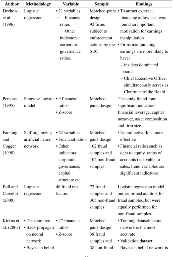
Table 2 summarizes the research methodology and findings of the FFR empirical studies most relevant to our study. The research methodology has shown a trend with an emphasis on the classification mechanization which is used as the decision support information for future risk identification (Basens et al., 2003).
Table 2. Research methodology and findings in FFR empirical studies.
Author Methodology Variable Sample Findings
Dechow et al. (1996) Logistic regression • 21 variables – Financial ratios – Other indicators: corporate governance ratios. Matched-pairs design: 92 firms subject to enforcement actions by the SEC • To attract external
financing at low cost was found an important motivation for earnings manipulation
• Firms manipulating
earnings are more likely to have:
- insiders dominated boards
- Chief Executive Officer simultaneously serves as Chairman of the Board Persons (1995) Stepwise logistic model • 9 financial ratios • Z-score Matched- pairs design
The study found four significant indicators: financial leverage, capital turnover, asset composition and firm size
Fanning and Cogger (1998) Self-organizing artificial neural network • 62 variables • Financial ratios • Other indicators: corporate governance, capital structure etc. Matched- pairs design: 102 fraud samples and 102 non-fraud samples
• Neural network is more effective
• Financial ratios such as debt to equity, ratios of accounts receivable to sales, trend variables are significant indicators Bell and Carcello (2000) Logistic regression 46 fraud risk factors 77 fraud samples and 305 non-fraud samples
Logistic regression model outperformed auditors for fraud samples, but were equally performed for non-fraud samples. Kirkos et al. (2007) • Decision tree • Back-propagati on neural network • Bayesian belief • 27 financial ratios • Z-score Matched- pairs design: 38 fraud samples and 38 non-fraud
• Training dataset: neural network is the most accurate
• Validation dataset:
network samples the most accurate Hoogs et al. (2007) Genetic Algorithm • 38 financial ratios • 9 qualitative indicators 51 fraud samples vs. 51 non-fraud samples
Integrated pattern had a wider coverage for suspected fraud companies while it remained lower false classification rate for non-fraud ones Source: (Hsu, 2008; Huang et al., 2011).
As shown in Table 2, Persons (1995) used Stepwise logistic model to found significant indicators relate to FFR. Dechow et al. (1996) used Logistic regression in FFR detection. Bell and Carcello (2000) developed a Logistic regression model useful in predicting the existence of fraudulent financial reporting, and found that the proposed model outperformed auditors for fraud samples, but were equally performed for non-fraud samples.
Green and Choi (1997) applied Back-propagation neural network to FFR detection. The model used five ratios and three accounts as input. The results showed that Back-propagation neural network had significant capabilities when used as a fraud detection tool. Fanning and Cogger (1998) proposed a generalized adaptive neural network algorithm, named AutoNet, to FFR detection. The input vector consisted of financial ratios and qualitative variables. They compared the performance of their model with linear and quadratic discriminant analysis, as well as logistic regression, and claimed that AutoNet is more effective at detecting fraud than standard statistical methods. Kirkos et al. (2007) compared Decision tree, Back-propagation neural network, and Bayesian belief network in FFR detection and found that Back-propagation neural network is the most accurate method in training dataset, Bayesian belief network is the most accurate method in validation dataset. Hoogs et al. (2007) applied Genetic Algorithm (GA) in FFR detection, and the performance of GA concluded that the integrated pattern had a wider coverage for suspected fraud companies while it remained lower false classification rate for non-fraud ones.
Humpherys et al. (2010) developed a linguistic methodology for detecting fraudulent financial statements. The results demonstrate that linguistic models of deception are potentially useful in discriminating deception and managerial fraud in
financial statements. Their findings provide critical knowledge about how deceivers craft fraudulent financial statements and expand the usefulness of deception models beyond a low-stakes, laboratory setting into a high-stakes, real-world environment where large fines and incarceration are the consequences of deception. In literature of financial fraud detection (FFD), Ngai et al. (2010) have done a complete classification framework and an academic review of literature which used data mining techniques for FFD. They showed that the main data mining techniques used for FFD are logistic models, neural networks, the Bayesian belief network, and decision trees, all of which provide primary solutions to the problems inherent in the detection and classification of fraudulent data. Huang et al. (2011) used the GHSOM to help capital providers examine the integrity of financial statement. They applied the GHSOM to analysis financial data and demonstrate an alternative way to help capital providers such as lenders to evaluate the integrity of financial statements, a basis for further analysis to reach prudent decisions. Huang and Tsaih (2012) evolved the GHSOM into a prediction model for detecting the FFR. They proposed the initial concept of a dual approach for examining whether there is a certain spatial relationship among fraud and non-fraud samples, identifying the fraud counterpart of a non-fraud subgroup, and detecting fraud samples.
The relevant literatures show that the neural network families have been widely used in many financial applications, such as the FFR detection, credit ratings, economic forecasting, risk management, or other FFD related issues.
2.5 Summary
The GHSOM is an improved vision of SOM. It is often used as a clustering tool and has proved its availability to deal with classification and clustering problem to achieve the decision support purpose. As a clustering tool, the related GHSOM studies nowadays still provide limit information (or lack of the inherent knowledge) from the clustering results, which may increase decision makers’ efforts to analyze such semi-structured results.
As a result, further analysis for the generated subgroups is needed. A particular design of the GHSOM for FFD is also needed since the learning nature of the GHSOM
is unsupervised. Recent researches which considered feature extraction or pattern recognition of the GHSOM are often applied to graphic data, sensor-collected data, or text content; however, few of studies have focus on financial data. Despite the GHSOM provides more delicate clustering results than the SOM, we find that no study has applied the GHSOM and integrated it into a DSS that helps identify fraud (e.g., FFR). Therefore, this study expects to utilize the advantage of the GHSOM to design a novel dual approach and apply it to detect FFR (a sub-field of FFD) that helps identify fraud cases and explore their imbedded features through the PCA and explore their potential FFR patterns through any qualitative method, and finally provides abundant detection results as the investigative report to facilitate the decision process of both identification and interpretation.
3. The proposed dual approach
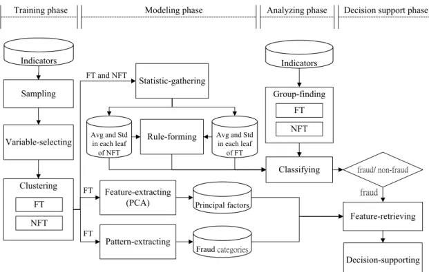
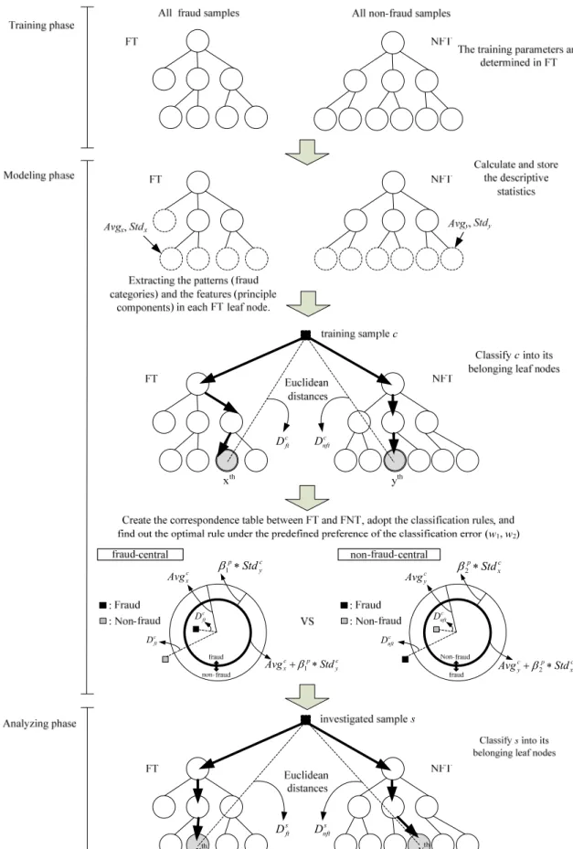
The overall system architecture of the proposed dual approach is illustrated in Figure 5. The proposed dual approach consists of the following four phases: the training, the modeling, the analyzing, and the decision support. There are eleven major modules: sampling, variable-selecting, clustering, statistic-gathering, rule-forming, feature-extracting, pattern-extracting, classifying, analyzing, feature-retrieving, and decision-supporting.
The training phase consists of a series of three modules, which aims to sequentially sample the data, select the input variables, and set up two GHSOM trees based upon the dichotomous categories of training samples. The modeling phase consists of a series of four modules, which aims to calculate two statistical values (Avg and Std) from each leaf node of the obtained two GHSOM trees to form the optimal classification rule based on the training samples, and extract features using quantitative and qualitative method from the GHSOM tree which consists of fraud samples. In other word, the modeling phase mainly focuses on setting up the classification rule based on certain spatial relationship, which match each leaf node of FT to its counterpart leaf nodes in NFT and vice versa.
The analyzing phase consists of two modules, in which the set GHSOMs, the classification rule and the extracted features are used to identify fraud from the unknown investigated samples, and retrieve the associated features for decision aid. Each investigated sample will be classified into its belonging leaf node of GHSOMs. Then, the optimal classification rule will be used to classify the investigated sample. The decision support phase consists of two modules, which present the classification result and retrieve the fraud related features for decision aid. For an investigated sample, if the classification result is fraud, the regularity of its belonging leaf node of FT, that is the principal components and the potential fraud categories, are retrieved.
Sampling
Variable-selecting
Clustering
Statistic-gathering Indicators
Modeling phase Analyzing phase
Feature-retrieving Group-finding Training phase Feature-extracting (PCA) Avg and Std in each leaf of NFT Avg and Std in each leaf of FT Rule-forming
Classifying fraud/ non-fraud
Decision-supporting fraud Principal factors Fraud categories Indicators Pattern-extracting
Decision support phase
FT NFT FT FT FT and NFT FT NFT
Figure 5. System architecture of the proposed dual approach.
Note: The clustering module generates two GHSOM trees. One is FT (use fraud samples), and the other one is NFT (use non-fraud samples). The group-finding module classifies the investigated sample into FT and NFT, respectively.
3.1 Training phase
Table 3 shows the training phase, in which the task of data pre-processing is done via step 1 and step 2. Step 2 can apply any variable selection tool such as the discriminant analysis, logistic model, and so forth.
Since fraud and non-fraud samples will be used to set up two GHSOM trees (named non-fraud tree, NFT, and fraud tree, FT) respectively, before processing step 3, the training samples are grouped as the fraud ones and the non-fraud ones. In step 3, the fraud samples are used to set up an acceptable GHSOM named FT. After identifying the FT, the values for (the GHSOM’s) breadth parameter (τ1) and depth
parameter (τ2) are determined and stored in step 4. Then, in step 5, the determined
values of τ1 and τ2 and the non-fraud samples are used for setting up another GHSOM
Table 3. The training phase.
3.1.1 Sampling module
The sampling module processes sample collection and variable measurement. The sampling module is executed via the step 1 of Table 3. The definition of a fraud sample and a non-fraud sample are defined first. The sources, the sample period and the way of sampling are also decided in this step. The design of the sampling process is flexible depended on the application field.
The explanatory variables are selected based upon fraud related literatures. These measurements may proxy for several attributes of a sample. The next step will help to select variables significantly relate to fraud, which help downsize the number of input variables to make it more relevant to the collected sample base.
3.1.2 Variable-selecting module
The variable-selecting module is executed via the step 2 of Table 3. In the variable-selecting module, the collected explanatory variables and the fraud/non-fraud dichotomous dependent variable are put into the variable selection tool. Any variable selection tool such as discriminant analysis, logistic model, and so forth can be applied in this step. For example, in this study, the variable-selecting module applies discriminant analysis processing variable selection from the obtained samples in order to identify the significant variables that help detect fraud. Then, the variables with statistically significant effects will be chosen as the input variables for GHSOM training to obtain clustered groups.
step 1: Sample and measure variable.
step 2: Identify the significant variables that will be used as the input variables.
step 3: Use the fraud samples to set up an acceptable GHSOM (denote FT). step 4: Based upon the accepted FT, determine the (GHSOM training)
parameters breadth (τ1) and depth (τ2).
step 5: Use the non-fraud samples and the determined parameters τ1 and τ2 to
3.1.3 Clustering module
The clustering module is executed via the step 3, step 4 and step 5 of Table 3. The significant variables derived from the variable-selecting module are used as the input variables for the GHSOM training to conduct clustering procedure. Two GHSOMs (named non-fraud tree, NFT, and fraud tree, FT) are respectively generated from two classes of training samples (fraud class, non-fraud class). For each GHSOM, a series of leaf nodes (i.e., groups) are generated. Furthermore, based upon the FT, we can get several clustered groups with inherent similarity for helping further feature extraction.
The competitive learning nature of GHSOM makes it work as a regularity detector that is supposed to discover statistically salient features of the sample population (Rumelhart and Zipser, 1985). In this module, the GHSOM will develop the topological representation which captures the most salient features of each cluster. Furthermore, through a set of small-sized leaf nodes, the GHSOM classifies the sample into more subgroups with hierarchical relations instead of a dichotomous result and therefore further delicate analyses are feasible.
3.2 Modeling phase
Table 4 presents the modeling phase, in which the classification rule is set up. Despite FT and NFT are resulted from fraud and non-fraud samples respectively, the spatial relationship hypothesis and the same setting of (τ1 and τ2) parameters may
render true that each leaf node of NFT has one or more than one counterpart leaf nodes in FT and vice versa. Thus, one purpose of the modeling phase is to match each leaf node of FT to its counterpart leaf nodes in NFT and vice versa.
Table 4. The modeling phase. step 1: For each leaf node of FT,
i. calculate and store its Avgx value that is the average of Euclidean
distances between the weight vector and the grouped fraud training samples;
Euclidean distances between the weight vector and the grouped fraud training samples.
step 2: For each leaf node of NFT,
i. calculate and store its Avgy value that is the average of Euclidean
distances between the weight vector and the grouped non-fraud training samples;
ii. calculate and store its Stdy value that is the standard deviation of
Euclidean distances between the weight vector and the grouped non-fraud training samples.
step 3: For each training sample,
i. identify and store the winning leaf node of FT and the winning leaf node of NFT, respectively;
ii. store its Avg values of the winning leaf nodes of FT and NFT,
respectively;
iii. store its Std values of the winning leaf nodes of FT and NFT,
respectively.
iv. calculate and store its Dft, the Euclidean distance between the
training sample and the weight vector of the winning leaf node of FT;
v. calculate and store its Dnft, the Euclidean distance between the
training sample and the weight vector of the winning leaf node of NFT.
step 4: Create the spatial correspondence tables regarding the matching from NFT to FT and from FT and NFT, respectively.
step 5: Use the fraud-central rule defined in Equation (3) and the optimization problem (4) to determine the parameter p
1
β that minimizes the corresponding sum of (type I and type II) classification errors. step 6: Use the non-fraud-central rule defined in Equation (7) and the
optimization problem (8) to determine the parameter p
2
β that minimizes the corresponding sum of (type I and type II) classification errors.
step 7: Pick up the dominant classification rule via comparing the classification errors obtained in step 5 and step 6.
step 8: For each leaf node of FT, apply PCA to select features through extracting factors (i.e., principle components).
step 9: For each leaf node of FT, analyze the common fraud features from exogenous information based on the associated domain categories.