Supercooled vortex liquid and quantitative theory of melting of the flux-line lattice in type-II superconductors

(1)

Supercooled vortex liquid and quantitative theory of melting of the flux-line lattice

in type-II superconductors

Dingping Li1,2_{and Baruch Rosenstein}2,3

1_{Department of Physics, Peking University, Beijing 100871, China}

2_{National Center for Theoretical Sciences and Electrophysics Department, National Chiao Tung University, Hsinchu 30050,} Taiwan, Republic of China

3_{Department of Condensed Matter Physics, Weizmann Institute of Science, Rehovot 76100, Israel}

(Received 12 May 2003; revised manuscript received 10 May 2004; published 28 October 2004)

A metastable homogeneous state exists down to zero temperature in systems of repelling vortices. A zero-“fluctuation-temperature” liquid state therefore serves as a(pseudo) “fixed point” controlling the properties of vortex liquid below and even around melting point. Based on this picture for the vortex phase we apply the Borel-Pade resummation technique to develop a quantitative theory of the vortex liquid for the lowest-Landau-level Ginzburg-Landau model in type-II superconductors. While on the solid phase, there exists a superheat solid phase which ends at the spinodal line. The picture for the vortex phase is supported by an exactly solvable large N Ginzburg-Landau model in a magnetic field and has been recently confirmed by the experiments. The applicability of the lowest-Landau-level model is discussed and corrections due to higher levels are calculated. The melting line is located based on the quantitative theory for the description of the vortex solid and the vortex liquid. Magnetization, entropy, and specific heat jumps along the melting line are calculated. The theoretical results explain quantitatively very well the experimental data on the high-Tccuprates YBa2Cu3O7,

DyBCO, low-T_cmaterial(K, Ba) BiO₃, and also Monte Carlo simulation results.

DOI: 10.1103/PhysRevB.70.144521 PACS number(s): 74.25.⫺q, 74.40.⫹k, 74.25.Ha, 74.25.Dw

I. INTRODUCTION

Abrikosov flux lines(vortices) created by magnetic field in type-II superconductors strongly interact with each other, creating highly correlated configurations like the vortex lat-tice. In high-Tc cuprates thermal fluctuations at relatively

large temperatures are strong enough to melt the lattice. Sev-eral remarkable experiments demonstrated that the vortex lattice melting in high-Tcsuperconductors is first order with

magnetization jumps1 _{and spikes in specific heat.}2 Magneti-zation and entropy jumps were measured using local Hall probes,1 _{superconducting quantum interference device,}3,4 (SQUID), torque magnetometry,5,6 _{and integrating the} spe-cific heat spike.2,7It was found that in addition to the spike there is also a jump in specific heat in YBa2Cu3O7(YBCO) which was measured as well.2,7,8 _{These precise} measure-ments pose the question of an accurate quantitative theoreti-cal description of thermal fluctuations in vortex matter.

The melting line in high-Tc cuprates has been studied

mainly not very far from Tc. In this part of the phase diagram

the Ginzburg-Landau(GL) approach is generally appropriate to describe thermal fluctuations near T_c.9,10_{The GL model is,} however, highly nontrivial even within the lowest-Landau-level (LLL) approximation valid at relatively high fields. This simplified model has only one parameter: the dimen-sionless LLL scaled temperature aT⬃关T−Tmf共H兲兴/共TH兲2/3

[defined precisely in Eq. (13) below]. Over the last 20 years a great variety of theoretical methods were applied to study this model. Brezin, Nelson, and Thiaville11_{applied the} renor-malization group(RG) method to the one-loop-level descrip-tion of the vortex liquid. No nontrivial fixed points of the (functional) RG equations were found and they concluded therefore that the transition from liquid to solid is first

order.12Another often-used approach applicable also beyond the range of validity of the GL model is to use an elasticity theory description of the vortex lattice and Lindermann cri-terion to determine the location of melting line.13 _However, all those approaches do not provide a quantitative theory of melting since these are one-phase theories and in order, for example, to calculate discontinuities at first-order transitions an accurate description of both phases is necessary.

Two perturbative approaches were developed and greatly improved recently to describe both the solid and liquid phases in the LLL GL model. The perturbative approach on the liquid side was pioneered long ago by Ruggeri and Thouless.14_{They developed a perturbative expansion around} a homogeneous(liquid) state in which all the “bubble” dia-grams are resumed. Unfortunately they found that the series are asymptotic, and although a first few terms provide accu-rate results at very high temperatures, the series becomes inapplicable for aTless than −2, which is quite far above the

melting line (believed to be located around aT⬃−10). We

recently obtained an optimized Gaussian series15 _{which is} convergent rather than asymptotic with radius of conver-gence of aT= −5, but it is still unfortunately above the

melt-ing point.

For the vortex solid in the LLL GL mode, Eilenberger16 and Maki and Takayama16 _{calculated the fluctuations} spec-trum around Abrikosov’s mean-field solution. They noticed that the vortex lattice phonon modes are softer than that of the acoustic phonons in atomic crystals and this leads to infrared(IR) divergences in certain quantities. This was ini-tially interpreted as the “destruction of the vortex solid by thermal fluctuations” and the perturbation theory was aban-doned. However, the divergences look suspiciously similar to “spurious” IR divergences in the critical phenomenon theory

(2)

and recently it was shown that all these IR divergences can-cel in the perturbative series for physical quantities, in par-ticular the effective free energy.17 _{The perturbative series} therefore is reliable and was extended to two loops for the free energy. The free energy calculated to two loops on the solid side is now precise enough even around the melting point.

Therefore the missing part is a theory in the region −10⬍aT⬍−5 for the liquid phase. Moreover, this theory

should be very precise since free energies of solid and liquid happen to differ only by a few percent around melting. Closely related to melting is the problem of the nature of the metastable phases of the theory. While it is clear that the overheated solid becomes unstable at some finite tempera-ture, it is not generally clear whether the overcooled liquid in the LLL GL model becomes unstable at some finite tempera-ture(like water and other molecular liquids, which, however, have a crucial attractive component of the intermolecular force) or exists all the way down to T=0 as a metastable state. The Gaussian (Hartree-Fock) variational calculation, although perhaps of a limited precision, is usually a very good guide as far as the qualitative features of the phase diagram are concerned. Such a calculation in the liquid was performed long ago,14 _{while a significantly more} compli-cated one sampling also inhomogeneous states (vortex lat-tice) was obtained recently.18,19_{The Gaussian results are as} follows. The free energy of the solid state is lower than that of the liquid for all temperatures lower than melting tempera-ture a_Tm. The solid state is therefore the stable one below a_Tm, becomes metastable at somewhat higher temperatures, and is destabilized at aT= −5.5. The liquid state becomes metastable

below the melting temperature, but unlike the solid, does not lose metastability all the way down to a_Tm= −⬁ 共T=0兲. The excitation energy of the supercooled liquid approaches zero as a power␧⬃1/a_T2. This general picture is supported in Sec. III by an exactly solvable large N Ginzburg-Landau model of vortex matter in type-II superconductors.

In the meantime similar qualitative results were obtained in different area of physics. It was shown by variety of ana-lytical and numerical methods that liquid(gas) phase of the classical one component Coulomb plasma exists as a meta-stable state down to very low temperature, possibly T = 0.20 The quantum one-component plasma-electron gas also shows similar features.21_{It seems plausible to speculate that} the same phenomenon would happen in any system of point-like or linepoint-like objects interacting via purely repulsive forces. In fact the vortices in the London approximation are a sort of repelling lines with the force even more long range than Coulombic. This was an additional strong motivation to con-sider the above scenario in vortex matter. In addition to the above-mentioned theoretical evidence for the validity of the scenario, very recently, the supercooled vortex liquid at very low temperature and the superheat vortex solid which van-ishes at spinodal line have been observed in a beautiful ex-periment on 2H-NbSe2 by Xiao et al.22 Previous experiments23 _{showed that the observed effect is not due to} surface pinning or geometrical barriers.

Assuming the absence of singularities on the liquid branch allows us develop an essentially precise theory of the LLL GL model for vortex liquid(even including supercooled

liquid) using methods of theory of critical phenomena.24,25 The generally effective mathematical tool to approach a non-trivial fixed point (in our case at zero temperature) is the Borel-Pade(BP) transformation.25_{Before embarking on this} program in the following sections, we address several subtle-ties which prevented the use and acceptance of the BP method in the past. Very early on Ruggeri and Thouless14 tried to use BP(unfortunately a “constrained” one, so that it interpolates smoothly with the solid, an assumption we be-lieve is incorrect) to calculate the specific heat without much success. It was shown by Wilkin and Moore26 _{that the} con-strained BP does not converge, while the results for uncon-strained BP were inconclusive. They attributed this to the limited order of expansion known at that time. The BP liquid theory combining with the recently developed LLL theory of solids could be used to calculate the melting line and the magnetization and the specific heat jumps across the line.27 The attempts to use BP for the calculation of the melting line using a longer series also ran into problems. Hikami, Fujita, and Larkin27_{tried to find the melting point by comparing the} BP liquid free energy with the one-loop solid free energy and obtained aT= −7. However, their one-loop solid energy was

incorrect and, in any case, it was not precise enough(as will become clear in the following discussions that the two-loop contribution cannot be neglected).

The LLL GL model has been studied by various methods. For example, it was also studied numerically in both the Lawrence-Doniach model [a good approximation of the three-dimensional(3D) GL for large number of layers] (Refs. 28 and 29) and in 2D (Ref. 30) and by a variety of nonper-turbative analytical methods, among them the density functional,31 _{1 / N,}32–34 _{dislocation theory of melting,}35 _and others.36_{However, most of those theories in the literature are} qualitative and have not given us a quantitative description (locations of melting lines, magnetization jumps, entropy jumps, etc.) for the melting of vortex lattice. The theory we will describe in this article can face the experimental test and we found that the predication and results from the theory is in good quantitative agreement with experiments.

As we show in this paper, the BP liquid free energy com-bined with the correct two-loop solid energy computed re-cently gives scaled melting temperature a_Tm= −9.5 and in ad-dition predicts other characteristics of the model. The magnetization of liquid is larger than that of solid by ap-proximate 1.8% irrespective of the melting temperature(the specific heat jump is about 6% and decreases slowly with temperature in YBCO). A brief account of these results was published.18

In addition to the theory of melting, we considered over-cooled liquid and calculated magnetization and specific heat curves. Since the metastable overcooled liquid state exists all the way down to zero temperature in the model, we can define the liquid Madelung energy. Looking at the melting process from the low-temperature side for both the liquid and solid we find that the Madelung energy of the liquid is larger than that of the solid approximately by the latent heat of melting. Our magnetization curves agree quite well with Monte Carlo simulations of the LLL GL(Ref. 28) and almost perfectly for the specific heat in 2D by Kato and Nagaosa in Ref. 30.

(3)

We study also in this paper several “phenomenological” issues, some matter of significant disagreement. First is the range of applicability of the LLL model. We find that in order to describe the experimental reversible magnetization of YBCO at lower fields, higher-Landau-levels (HLL) cor-rections should be incorporated. We therefore clarify in Sec. V the role of the HLL modes. Experimentally it was claimed that one can establish the LLL scaling for fields above 3T.37 A glance at the data, however, shows that in normal state (above Tc) the LLL scaling for magnetization curves is

gen-erally very bad. Most of the HLL effects can be taken into account by just renormalizing the parameters of the LLL model. Therefore one should use the “effective LLL” in which HLL were “integrated out.” To clarify this often-salient feature we explicitly perform this integration within a self-consistent approach in Sec. V. It was noted by Koshelev38 _{and others that, to calculate magnetization, one} has to carefully account for renormalization of the free en-ergy since it is field dependent. Then we calculated the lead-ing correction to the effective LLL and compare it with ex-periments. It is found that although the LLL contribution to magnetization is much larger that the experimentally ob-served one above Tc, it is nearly canceled by the HLL

con-tributions. This explains the breaking of the LLL scaling in the normal state.

The paper is organized as follows. The model is defined and its applicability range discussed in Sec. II. In Sec. III, the (including supercooled) liquid and (including superheated) solid in the LLL GL will be discussed in the mean-field approximation of the LLL GL model and in the large-N LLL GL model. In Sec. IV, the LLL model is solved and the melting theory of vortex lattice is presented and compared to experiments. In Sec. V, the HLL corrections are discussed and the magnetization curves are compared with experi-ments.

In particular phenomenological issues are addressed in Secs. II B (assumptions), IV C (melting line, Ginzburg pa-rameter fit for various materials), IV D (magnetization, en-tropy jumps), IV E (specific heat jumps), and V D (reversible magnetization curve), so readers not interested in theoretical details can go directly to these sections.

II. GL MODEL AND ITS BASIC ASSUMPTIONS A. GL model

On the mesoscopic scale, 3D superconducting materials, with not very strong asymmetry along the z axis which we call as YBCO-type superconductors, are effectively de-scribed by the Ginzburg-Landau free energy functional

F关␺,␺* ,A兴 =

冕

d3x ប 2 2mab 兩D␺兩2₊ ប 2 2mc 兩⳵z␺兩2− a共T兲兩␺兩2 +b

⬘

2兩␺兩 4₊共B − H兲 2 8␲ 共1兲

involving the order parameter field␺ and magnetic field B. The external constant magnetic field is described by the vec-tor potential in Landau gauge A0=共Hy,0,0兲. The covariant

derivative is defined by D⬅ ⵱−2␲iA /⌽₀,⌽₀⬅hc/e* 共e* = 2e兲. The microscopic thermal fluctuations are integrated out and, as a consequence, coefficients a, b

⬘

, and m depend on temperature. Mesoscopic thermal fluctuations of the order parameter are described by the partition function

Z =

冕

D␺D␺*DA exp

再

−F关␺,␺* ,A兴

T

冎

. 共2兲

Our aim is to quantitatively describe the effects of thermal fluctuations of high-Tccuprates of the YBCO type.

B. Assumptions

The use of the above GL free energy hinges upon several physical assumptions. They are listed below.

(i) Continuum 3D model. We use the anisotropic GL model despite the well established layered structure of the high Tccuprates for which models of the Lawrence-Doniach

type are more appropriate. Effects of layered structure are dominant in BSCCO or Tl compounds (anisotropy very large:␥⬅

冑

mc/ mab⬎1000) and noticeable for cuprates with

anisotropy of order ␥= 50 like LaBaCuO, strongly under-doped YBCO (see, however, Ref. 39), or Hg1223. The re-quirement that the 3D GL model can be effectively used therefore limits us to optimally doped YBCO7−␦ (or slightly overdoped or underdoped) for which the anisotropy param-eter is not very large[around␥= 4 – 8(Ref. 40)], DyBCO and possibly Hg1221 which has a slightly larger anisotropy. However there is no such problem in recently discovered isotropic “fluctuating” superconductor(K, Ba) BiO3.41

(ii) Range of validity of the mesoscopic (GL) approach. The GL approach generally is an effective mesoscopic ap-proach. It is applicable when one can neglect higher-order terms in the functional of Eq.(1), typically generated when one “integrates out” microscopic degrees of freedom. The leading higher-dimensional terms we neglect (as “irrel-evant”) are 兩␺兩6 _{and higher} _{(four) derivative terms like} 兩D2_␺_兩2_{. This naively leads to a condition that 1 − t − b is} smaller than 1. Here and in what follows, one defines

t⬅ T/Tc, b⬅ B/Hc2⬇ H/Hc2⬅ h. 共3兲

The applicability line 1 − t − b⬍0.2 for YBCO is plotted in Fig. 1. We also will consider a model invariant under rota-tions in the ab plane. Noninvariant models sometimes can be rescaled to ma⯝mb= mab.10. For several physical questions

those assumptions are not valid because neglected “irrel-evant” terms might become “dangerous.” For example the question of the structural phase transition into the square lattice is clearly of this type.42It is known that even assum-ing ma/ mb= 1 in low-temperature vortex lattices in YBCO,

rotational symmetry is broken down to the fourfold symme-try by the four derivative terms. However, there is no signifi-cant correction to other physical quantities—for example, the magnetization from those higher-dimensional terms.

(iii) Expansion of parameters around Tc. Generally the

parameters of the GL model of Eq.(1) are complicated func-tions of temperature which are determined by the details of the microscopic theory. We expand the coefficient a共T兲 near Tc:

(4)

a共T兲 = T_c关␣共1 − t兲 −␣

⬘

共1 − t兲2₊ _{¯ 兴.} _共4兲 The second and higher terms in the expansion are omitted and therefore, when temperature deviates significantly from Tc, one cannot expect the model to have a good precision.

We note that recently measured Hc2共T兲 is linear in T in a

wide region near Tcin both YBCO and共K,Ba兲BiO3.41,43 (iv) Constant nonfluctuating magnetic field. For strongly type-II superconductors like the high-Tccuprates not very far

from Hc2共T兲 (this easily covers the range of interest in this

paper; for the detailed discussion of the range of applicability beyond it see Ref. 44), the magnetic field is homogeneous to a high degree due to superposition from many vortices. In-homogeneity is of order 1 /␬2_⬃10−3_{. Since the main subject} of this study is thermal fluctuation effects of the order pa-rameter field, one might ask whether thermal fluctuations of the electromagnetic field should be also taken into account. Halperin, Lubensky, and Ma considered this question long time ago.45_{The conclusion was that they are completely} neg-ligible for very large ␬. Upon discovery of the high-Tc

cu-prates, the issue was reconsidered46_{and the same result was} obtained to a very high precision. Therefore here magnetic field is treated both as constant and nonfluctuating 共B=H兲 and the last term in Eq.(1) can be omitted (to precision of order 1 /␬2). However, when we calculate the magnetization M =共B−H兲/4␲, which is of order 1 /␬2, a higher-order cor-rection must be considered.

Recently it was claimed that the “vortex loop” fluctua-tions are important and even might lead to additional phase transition at field of order Gi Hc2.47 This is of order 100 G

for the materials of interest listed in Table II and therefore is irrelevant for physics discussed in this paper. Note that Gi in the papers discussing the vortex loops physics48 _{is assumed} to be much larger. We discuss this issue in Sec. IV C.

(v) Disorder. Point like disorder is always present in Y BCO. For example magnetization becomes irreversible. The melting line of the optimally doped or underdoped samples bends towards lower fields7 _{and signs of the second-order} transition appear at 12T.49 _{However, in some samples like}

fully oxidized YBa₂Cu₃O₇(Ref. 6) and DyBa₂Cu₃O₇ (Refs. 8 and 50) the disorder effects are minor especially at tem-perature close to Tc. In the maximally oxidized YBCO,6 the

second-order transition associated with disorder is not seen even at the highest available fields共30 T兲. Certain aspects of the disorder problem were addressed in the framework of GL theory,51 elasticity theory,52 and a phenomenological ap-proach based on the Lindermann criterion.13

Throughout the most of the paper, we will use the coher-ence length␰=

冑

ប2/共2mab␣Tc兲 as a unit of length, Tcas unit

of temperature, and关dHc2共Tc兲/dT兴Tc=⌽0/ 2␲␰2as a unit of magnetic field. As we mentioned above, we assume constant magnetic induction B = bHc2which is slightly different from

the external magnetic field H = hHc2. After rescaling Eq.(1)

by x→␰x, y→␰y, z→␰z /␥, and ␺2_→共2_␣_T

c/ b

⬘

兲␺2共␥

⬅

冑

mc/ mab兲 one obtains the Boltzmann factor

f =F T= 1 ␻

冕

d 3_x

冋

1 2兩D␺兩 2₊1 2兩⳵z␺兩 2₋

冉

_a h+ b 2

冊

兩␺兩 2 +1 2兩␺兩 4₊␬ 2_{共b − h兲}2 4

册

, 共5兲

where the dimensionless parameter

␻=

冑

2NGi␲2t 共6兲 characterizes the strength of thermal fluctuations and the res-caled D⬅ ⵱−iA with A=共by,0,0兲. The commonly used di-mensionless Ginzburg number is defined by

N_Gi⬅ 1 2

冉

32␲e2␬2␰Tc␥ c2h2

冊

2 . 共7兲 And ah= 1 − t − b 2 . 共8兲

defines the distance from the mean-field transition line.

C. Landau level modes in the quasimomentum basis Assuming that all the requirements are met, we now di-vide the fluctuations into the LLL and HLL modes to make the problem manageable. It is convenient to expand the order parameter field in a complete basis of noninteracting theory: the Landau levels. In the hexagonal lattice phase the most convenient basis is the quasimomentum basis

␺共x,y,z兲 =

_冑

1 2共2␲兲3/2

冕

k

兺

n=0 ⬁ e−ikzz␸ k n_共x,y兲_␺n_共k,k z兲. 共9兲

Here ␸_kn共x兲 is the eigenstate of the nth Landau level ␧n=共n+1/2兲b

关

1 2

兩

D␺

兩

2_␸ k n_{共x兲=共n+1/2兲b}_␸ k n_共x兲

兴

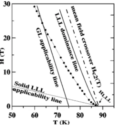
with two-dimensional quasimomentum k with hexagonal symmetry:

b− 2␲ a_⌬l

冊

2

冎

, 共10兲

where a_⌬⬅

冑

4␲/

冑

3. The function ␸A⬅␸k=0

n=0 _{describes the}

Abrikosov lattice solution.9_{Even in the liquid state, which is} more symmetric than the hexagonal lattice, we find it conve-nient to use this basis.

Naively, if the magnetic field is sufficiently high, the en-ergy gap of the order b separating the n = 0 LLL modes from the HLL is very large and it is reasonable to keep only the LLL modes in Eq.(5). The dominance of the LLL modes for melting was discussed in Ref. 11 and Pierson and Valls in Ref. 37, and we will discuss it in more detail in Sec. V. In the rest of this section, we consider the LLL GL model.

D. LLL scaling

Using the LLL condition兩D␺兩2= b兩␺兩2, the free energy is simplified: f = 1 ␻

冕

d 3_x

冋

1 2兩⳵z␺兩 2_{− a} h兩␺兩2+ 1 2兩␺兩 4₊␬ 2_{共b − h兲}2 4

d 3_x

冋

1 2兩⳵z␺兩 2_{+ a} T兩␺兩2+ 1 2兩␺兩 4 +␬2

冉

b␻ 4␲

冑

2

冊

−4/3_{共b − h兲}2 4

册

. 共12兲

Minimizing it with respect to b leads to magnetization b − h of the order of 1 /␬2. This means that in the strongly type-II limit 共␬Ⰷ1兲 the last term is of the order 1/␬2 and can be neglected. The theory has a single dimensionless parameter, the Thouless scaled temperature defined by

aT= −

冉

b␻ 25/2␲

冊

−2/3

ah. 共13兲

The Gibbs free energy density in the newly scaled model is defined as

g共aT兲 = −

4␲

冑

2

V log

冕

D␺D␺* exp兵− f关␺兴其, 共14兲 which is also a function of aTonly(4␲

冑

2 is the scaled

“tem-perature”). The relation to the original Gibbs free energy is G共T,H兲 = Hc2 2 2␲␬2

冉

b␻ 25/2_␲

冊

4/3 g共aT兲. 共15兲

III. OVERCOOLED LIQUID AND THE T = 0 FIXED POINT OF THE LLL MODEL

In this section, we will show that in the mean-field ap-proximation and the exact solvable large-N model, there is a zero-temperature pseudocritical point for the vortex liquid and the melting is a first-order phase transition. Moreover, there exists a superheat solid which ends at spinodal line.

The energy of the hexagonal solid in the mean field (ne-glecting mesoscopic thermal fluctuations) is9

g_Msol= − aT 2 2␤A , G_Msol= − Hc2 2 4␲␬2␤A a_h2, 共16兲 where␤A= 1.1596 and the subscript M underlies the

similar-ity to the Madelung energy of atomic solids. The major fluc-tuations contribution to the solid free energy is due to the “phonon” modes. In harmonic approximation it is propor-tional to the fluctuation temperature T = a_T−3/2:

g₁sol= 2.848兩a_T兩1/2_, _G 1 sol_{= C} 1 sol_T, _共17兲 C₁sol= 2.848Hc2B 8␬2Tc

冑

兩ah兩.

At low fluctuation temperatures one can neglect the T depen-dence of ah⯝−共1−b兲/2. The solid becomes unstable at aT

= −5.5 according to the self-consistent (Gaussian) approximation.19

In the (homogeneous) liquid state the order parameter vanishes and the contributions to the free energy come solely from fluctuations. The Gaussian (“mean-field”) approxima-tion to the free energy14_is

g = 4

冑

␧ − 4/␧, 共18兲 where the excitation energy ␧ is given by a solution of the cubic “gap equation”

␧3/2_{− a}

T

冑

␧ − 4 = 0. 共19兲

The liquid state becomes metastable below the melting tem-perature, but unlike the solid above melting, does not lose metastability at a certain “spinodal” point.54It persists all the way down to T = 0. The excitation energy of the supercooled liquid approaches zero as a power␧⬃16/a_T2. For aT→−⬁,

the scaled energy, Eq.(18), has an expansion in 1/a_T3⬀T2for small fluctuation temperature T(the radius of convergency of the expansion extending to aT= −3). Therefore the liquid

de-spite having energy larger than that of the solid becomes (pseudo)critical55 _{at zero temperature. Physical quantities} “around” this point exhibit a power behavior with character-istic (pseudo)critical exponents. The metastable liquid state has a distinct Madelung energy

gM liq = −aT 2 4, GM liq = − Hc2 2 8␲␬2ah 2 . 共20兲

As the temperature increases the difference between the solid and liquid becomes smaller and vanishes at melting. Gener-ally one expects a linear correction at small T:

(6)

Gliq= Gliq_M+ C₁liqT. 共21兲 Since the expansion of the mean-field free energy is in T2_, C₁liq= 0. Comparing the solid free energy, Eqs.(16) and (17), with Eq.(21), we get the melting temperature a_Tm= −6.3. We therefore conclude that in this approximation the supercooled liquid state exists down to its pseudocritical point at zero temperature. Moreover, the pseudocritical point might gov-ern the behavior of the liquid phase to temperatures as high as the melting point and there exists a good low-temperature expansion(stronger coupling expansion) for the supercooled liquid.

It is important to confirm the above scenario in an exactly solvable model. The simplest model of this kind is the mul-ticomponent GL model. The LLL GL theory can be general-ized (in several different ways) to an N-component order parameter field␺a, a = 1 , . . . , N: f = 1 4␲

冑

2

冕

d 3_x

冋

1 2兩⳵z␺ a_兩2_{+ a} T兩␺a兩2+ ␯ 2N兩␺ a_兩2_兩_␺b_兩2 +1 −␯ 2N ␺ a_␺a_␺*b_␺*b

册

_. _共22兲

The large-N limit of this theory can be solved in a way similar to that in the N-component scalar models widely used in theory of critical phenomena.24The simplest case␯= 1 has been considered in Ref. 32. It was found that the homoge-neous state is stable at all temperatures. Under assumption that the conventional Abrikosov lattice takes over at low temperatures it supported the original conjecture by Brezin et al.11 that melting of the flux lattice is a first-order phase transition. However, it was shown (by explicit numerical evaluation) in Ref. 12 that the low-temperature ground state in that model is not the Abrikosov lattice state in which just one component has a nonzero expectation value(similar to the one component Abrikosov lattice). The “true” ground state has infinite degeneracy. Different ground states at large N are markedly different from the hexagonal lattice. The case

␯= 2, in which the Abrikosov lattice state is a stable ground state, was first introduced in Ref. 34 and we will refer it as the Lopatin-Kotliar (LK) model. Equation (22) is a slight generalization including both models studied in Refs. 32 and 34. We find that in fact all models with␯艌2 possess such a stable lattice state.

A straightforward method to develop the 1 / N expansion with the last component of␺Nhaving the expectation value ⬀␸A⬅␸k=0

n=0_{, describing the hexagonal lattice} _{[see Eq. (10)],}

is to shift this field ␺N共x,y,z兲→␺N共x,y,z兲+

冑

Nc␸A共x,y兲,

where c is a(real) constant. Then one introduces Hubbard-Stratonovich (HS) fields ␳, ␹ (Ref. 34) via free energy f关␺a_,_␳_,_␹_{兴 equal to} 1 4␲

冑

2

冓

1 2兩⳵z␺ a_兩2₊_共_␯␳_{+ a} T兲兩␺a兩2+␯c2兩␸A兩2兩␺a兩2 +1 −␯ 2 关共c 2_␸ A 2₊_␹_兲_␺*b_␺*b_{+ c.c.}_兴

冔

The spectrum has two branches

⑀O,A共k兲 = aT+␯共␤kc2+␳k兲 ± 兩共1 −␯兲共c2␥k+␹k兲兩. 共26兲

To have a stable perturbative Abrikosov solution which shall be a good solution for the low temperature, the spectrum should be positive definite for␳_k=␹_k= 0(in the perturbative approach, ␳k=␹k= 0 and c2=兩aT兩/␤A). Thus we demand

−␯/ 2 +共␯− 1兲艌0 or␯艌2, as stated above. The HS fields ␳k=具␳共x兲兩␸k共x兲兩2典x, ␹k=具␹共x兲␸k *_共x兲_␸ −k * _共x兲典 x, 共27兲

and the constant c are determined by minimizing free energy gef f.

Now we will study the inhomogeneous (solid) solution. The minimization with respect to␳共x兲 and␹共x兲 leads to

␳共x兲 = 具兩␸k共x兲兩2兵关⑀O共k兲兴−1/2+关⑀A共k兲兴−1/2其典k sgn共1 −␯兲␹共x兲 =

冓

␸k共x兲␸−k共x兲 c2␥k+␹k 兩c2_␥ k+␹k兩兵关⑀O共k兲兴−1/2 −关␧A共k兲兴−1/2其

冔

k , 共28兲

which, in terms of Fourier harmonics of the hexagonal lat-tice, takes a form

␳l=具␤l−k兵关⑀O共k兲兴−1/2+关⑀A共k兲兴−1/2其典k sgn共1 −␯兲␹l=

冓

␥k,l * c 2_␥ k+␹k 兩c2_␥ k+␹k兩兵关⑀O共k兲兴−1/2−关⑀A共k兲兴−1/2其

冔

k . 共29兲 The lattice functions␤k,␥k, and␥k,lare defined as

␤k=具兩␸兩2␸k→␸_k→ * 典x, ␥k=具共␸*兲2␸−k→␸k→典x, ␩k=兩␹k兩,␥k,l=具␸k * ␸−k * ␸−l→␸l→典x, 共30兲

and their properties were discussed in more detail in Ref. 19. The only consistent solution preserving hexagonal symmetry is␹k=␹c␥kwhere␹cis a constant independent of kជ, and the

(7)

sgn共1 −␯兲␹c␤A=具sgn共c2+␹c兲␩k兵关⑀O共k兲兴−1/2−关⑀A共k兲兴−1/2其典k.

共31兲 For the LK model,34 ␯= 2, this leads to ␹c␤A

=具␩k兵关⑀A共k兲兴−1/2−关⑀O共k兲兴−1/2其典k. Finally the set of the

mini-mization equations(using the properties of the lattice func-tions␤k,␥k,␥k,l) can be derived:

0 = a_T+␤_Ac2+ 2具␤_k兵关⑀_O共k兲兴−1/2+关⑀_A共k兲兴−1/2其典_k +具␩k兵关⑀O共k兲兴−1/2−关⑀A共k兲兴−1/2其典k, ␹c␤A=具␩k兵关⑀A共k兲兴−1/2−关⑀O共k兲兴−1/2其典k, ␳l=具␤l−k兵关⑀O共k兲兴 −1/2₊_关_⑀ A共k兲兴 −1/2_其典 k, 共32兲 and ⑀O,A共k兲 = aT+ 2␤kc2+ 2␳k±兩共c2+␹c兲␥k兩. 共33兲

The following formulas can be obtained and used for the calculation of the free energy:

具␳2_{典 = 具}_␤ l−k兵关⑀O共k兲兴−1/2+关⑀A共k兲兴−1/2其兵关⑀O共l兲兴−1/2 +关⑀A共l兲兴−1/2其典k,l, 具兩␹兩2_{典 =} 1 ␤A 关具␩k兵关⑀A共k兲兴−1/2−关⑀O共k兲兴−1/2其典k兴2. 共34兲

Equation (32) can be solved very easily by using mode expansion and iteration method.19,34 _{The spectrum can be} written as follows:

⑀O共k兲 = E共k兲 + ⌬␩k, ⑀A共k兲 = E共k兲 − ⌬␩k, 共35兲

with E共k兲 expanded in modes:

E共k兲 =

兺

En␤n共k兲, 共36兲 where ␤k=

兺

n=0 ⬁ exp关− 2␲n/

冑

3兴␤n共k兲, ␤n共k兲 ⬅

兺

兩X兩2₌₄_␲n/冑₃ exp关ik · X兴, 共37兲 where X lies on the lattice which basic “cell” is a primitive cell of the vortex lattice and the integer n determines the distance of a lattice point from the origin. For some integers—for example, n = 2 , 5 , 6 —␤n= 0 and the first three

nonzero ␤n are ␤0,␤1,␤3. The effective “expansion param-eter” is exp关−2␲/

冑

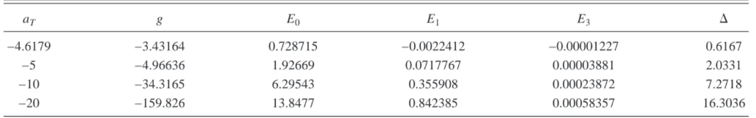
3兴=0.0265 and coefficients decrease

ex-ponentially with n.19 It is quite easy to get a more higher-mode approximation, but it is not necessary as the first few-mode approximation has given us a result with very high precision. As an example, when we retain the first three non-zero␤_nexpansion approximation, the result can be seen from Table I.

The solution disappears at aT= −4.6179. At this point the

solid is no longer a metastable state.⑀A共k兲 is a gapless mode

and⑀A共k兲→const⫻k2for k→0 in the large-N model.

How-ever, for the perturbative spectrum, ⑀A共k兲→const⫻k4 for

k→0. Using gef f N = aTc 2₊␤A 2 c 4₋

冓

_␳2₋1 2兩␹兩 2

冔

x + 2具

冑

⑀O共k兲 +

冑

⑀A共k兲典k, 共38兲 the energy corresponding to the solid solution of the minimi-zation equation(32) is given in Table I. The convergence of the mode expansion is exponential as seen from Table I.

For liquid, we impose the rotation-invariant ansatz with c2_{= 0,}_␹_{= 0 and obtain the gap equation}

␳=

_冑

2

a_T+ 2␳, 共39兲

which minimizes the energy

gliq= −␳2+ 4

冑

aT+ 2␳. 共40兲

The results for both the liquid and solid free energies are plotted in Fig. 2. The melting point appears at a_T= −5.15 where the liquid and solid energies are equal.

TABLE I. Coefficients of the mode expansion for the solid solution.

a_T g E₀ E₁ E₃ ⌬

−4.6179 −3.43164 0.728715 −0.0022412 −0.00001227 0.6167

−5 −4.96636 1.92669 0.0717767 0.00003881 2.0331

−10 −34.3165 6.29543 0.355908 0.00023872 7.2718

−20 −159.826 13.8477 0.842385 0.00058357 16.3036

FIG. 2. Free energy of solid(dotted points) and liquid (cross points) of the large-N model as function of the fluctuation tempera-ture 1 /兩aT兩3/2. The solid line ends at a point(dot), indicating the loss

(8)

It is well approximated in the whole region by its low-temperature expansion in powers of兩aT兩−3/2[which is

propor-tional to the “fluctuation temperature” T assuming that at low temperatures ah⯝−共1−b兲/2]: gsol a_T2 = cM sol + c1 sol T + c2 sol T2, . . . ,T⬅ 兩aT兩−3/2, csol_M = − 1 2␤A , c1 sol = 2.84835, c2 sol = − 2.54087. 共41兲 The first two terms of this large-N model are the same as for the usual one-component model, while the two-loop correc-tion is different.

Similarly the liquid energy can be expanded, but this time in powers of square of the “fluctuation temperature” T:

gliq a_T2 = cM

liq

+ c₁liqT + c₂liqT2, . . . ,T =兩aT兩−3/2,

c_Mliq= −1 4, c1,3,. . .

liq

= 0, c₂liq= 6, c₄liq= − 20. 共42兲 Here the first term is the “Madelung energy” of liquid at zero fluctuation temperature. Note that, as in the mean-field ap-proximation to the one-component theory, there is no term linear in T (the harmonic approximation). This means that the specific heat vanishes at zero temperature. Retaining just the Madelung and the harmonic term for solid and liquid we estimate the melting temperature in the linear approximation:

Tm=

c_Msol− c_Mliq

c₁liq− c₁sol. 共43兲 The latent heat in the same approximation is

⌬U = cM sol

− c_Mliq. 共44兲

Numerically this melting temperature Tm= 0.064

correspond-ing to aT= −6.25 and the latent heat ⌬U=0.18 should be

compared with the exact results: T_m= 0.086 共a_T= −5.15兲, ⌬U=0.122945. This shows that the low-temperature expan-sion of the supercooled liquid free energy gave us quite a sensible result.

In this section we obtain the first-order melting in the mean-field LLL GL model and the large-N LLL GL model. We note that as we show in last section, the GL model or the LLL GL model may not be valid for every low temperature. Thus in reality, the zero-temperature pseudocritical fixed point may not exist, though the LLL GL model does have this pseudocritical fix point at zero temperature. In the mean-field solution of the LLL GL model, the large-N LLL GL model and even the exact solution of the LLL GL model as we will show in the next section, supercooled liquid persists as a metastable state all the way to zero temperature and the superheat vortex solid exists and vanishes at the spinodal line. Based on the fact that the GL LLL model has a zero-temperature fixed point, we could use the Borel-Pade method to calculate the liquid free energy of the LLL GL model at higher temperature(see the next section for details). There-fore we can use this method to calculate the liquid free

en-ergy and use it within the validity region of the LLL model. We emphasize that this means that the matching of the (Borel-Pade approximant) liquid to the solid energy at T=0 employed in Ref. 14 to improve convergence of the series is not only ineffective,26_{but should lead to an incorrect result.} Liquid and solid energies are different in the limit of zero fluctuation temperature in this model.

In a recent experiments, Xiao et al. observed the super-cooled vortex liquid at very low temperature and the superheat vortex solid which vanishes at spinodal line in 2H-NbSe₂ by Ref. 22. They found that the spinodal line is around aT= −6 which is a bit higher than aT= −5.5 in the

Gaussian approximation calculation. This small discrepancy could attribute to the fact that Gaussian approximation is not very good for too small a_T.

In atomic liquids, an attractive long-range force is gener-ally present. As a result the supercooled liquid state loses its metastability at an end point (spinodal).54 _Lovett56 _{a long} time ago argued on general grounds(the stability analysis of approximate set of relations between density correlators) that for certain purely repelling interactions the spinodal point disappears (or, in other words, shifted to zero temperature) and is recovered when the attractive interaction is intro-duced. The existence of a metastable overcooled liquid down to zero temperature for repelling particles therefore might be quite general.

IV. BOREL-PADE METHOD APPLIED TO THE LLL MODEL: MELTING LINE, MAGNETIZATION,

AND SPECIFIC HEAT A. BP method applied to liquid energy

As we have seen above, within the mean-field approxima-tion of the LLL GL model or the large-N LLL GL model, the liquid branch exhibits a pseudocritical point55 _{at T = 0. It is} well known that in the theory of critical phenomena one can obtain an accurate description in the critical region by apply-ing the Borel-Pade method to the perturbation expansion at “weak coupling”.25 _{In technical terms there exists a} renor-malization group flow from the weak-coupling fixed point towards the strongly couple one.24We therefore start with the (renormalized) weak-coupling (high-temperature or nonideal gas) expansion.

The liquid LLL(scaled) free energy is written as14 g_liq= 4␧1/2_{关1 + h共x兲兴.} _共45兲 The function h can be expanded as

h共x兲 =

兺

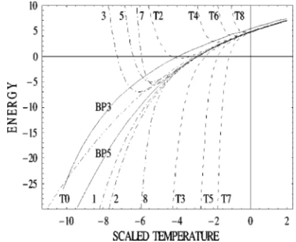
cnxn, 共46兲

where the “small parameter” x =1₂⑀−3/2and⑀is defined as a solution of the Gaussian gap equation(68). The coefficients cn can be found in Ref. 27. The consecutive approximants

are plotted in Fig. 3 as dashed lines (T1–T9, T0 being equivalent to the Gaussian mean field). One clearly sees that the series are asymptotic and can be used only at aT⬎−2.

One can improve on the Gaussian variational method by op-timizing the variational parameter⑀at each order instead of fixing it at the first-order calculation. The procedure is rather

(9)

involved(see Ref. 57). However, the optimized perturbation series is now convergent with radius of convergence about aT= −5(see dash-dotted lines 1–9 in Fig. 3). Finally we will

construct the BP series and compare them with the optimized perturbation series results for aT⬎−5.

We denote by hk共x兲 the 关k,k−1兴 BP transform25 of h共x兲

(other BP approximants violate the correct low-temperature asymptotics). The BP transform is defined as

hk=

冕

0 ⬁ h ˜ k共xt兲exp共− t兲dt, 共47兲

where ˜hk is the 关k,k−1兴 Pade transform of

兺n=1

2k−1_c

nxn/ n!—namely, a rational function 兺i=1 k _a

ixi/兺i=1 k−1_b

ixi

with the same expansion at small x as the original function. For k = 4 and k = 5, the liquid energy converges to required precision(0.1%); see Fig. 3. In this figure only k=3 and 5 are shown since k = 4 practically coincides with the latter. In what follows we will use h5as the best available approxima-tion of the liquid branch. The liquid energy completely agrees with the optimized Gaussian expansion results15_until its radius of convergence at aT= −5. We therefore conclude

that k = 5 is quite good for our purposes.

Since the metastable liquid state exists at all temperatures, one can consider the T = 0 limit. One finds

gliq共a_T兲 gsol共aT兲

→ 0.964 共48兲

for aT→−⬁. For gsol共aT兲, the leading term in this limit is

−a_T2/ 2␤A, which is the Madelung energy of the solid. The

leading term for gliq共aT兲 is −0.964aT

2

/ 2␤A. Usually the

Made-lung energy for the solid phase of the point particle system is realized by minimizing the potential energy of the system (the minimum is often obtained by taking the hexagonal lat-tice for the repulsive system in 2D). In this vortex system, we can have the supercooled liquid down to aT→−⬁ 共T

→0兲. The leading term for the overcooled liquid energy or

the Madelung energy of the liquid is therefore equal to

−0.964a_T2/ 2␤A, which is slightly larger than the Madelung

energy of the solid. This limit, the “ideal liquid,” however, cannot be thought as a minimization of a potential energy.

B. Melting line: Comparison with Monte Carlo simulations and Lindemann criterion

The solid energy calculated perturbatively to two loops is17,19 gsol= − a_T2 2␤A + 2.848兩aT兩1/2+ 2.4 aT , 共49兲

where␤_A= 1.1596. In Fig. 1 of Ref. 18 we plot the energies of the solid and liquid. They are very close near melting(see the difference on inset of this figure). We find that the melt-ing point(the energy curves of solid and liquid cross at the melting point) is

a_Tm= − 9.5. 共50兲

The available 3D Monte Carlo simulations28 _{unfortunately} are not precise enough to provide an accurate melting point since the LLL scaling is violated and one gets values of a_Tm = −14.5, −13.2, −10.9 at magnetic fields 共1,2,5兲T respec-tively. We found also that the theoretical magnetization cal-culated by using parameters given by Ref. 28. is in a very good agreement with the Monte Carlo simulation result of Ref. 28. However, the determination of melting temperature needs higher precision, and the sample size(⬃100 vortices) used in Ref. 28 may be not large enough to give an accurate determination of the melting temperature (due to boundary effects, LLL scaling will be violated too). The situation in 2D is better since the sample size is much larger. We performed similar calculation for the 2D LLL GL liquid free energy, combined it with the earlier solid energy calculation,17,19

gsol= − a_T2 2␤_A+ 2 log 兩aT兩 4␲2− 19.9 a_T2 − 2.92, 共51兲 and find that the melting point a_Tm= −13.2. It is in good agree-ment with MC simulations.30

Phenomenologically the melting line can be located using the Lindemann criterion or its more refined version using the Debye-Waller factor. The more refined criterion is more ap-propriate since vortices are not point like. It was found nu-merically for Yukawa gas58 _{that the Debye-Waller factor} e−2W_{(ratio of the structure function at the second Bragg peak} at melting to its value at T = 0) is about 60% at the melting point. Using methods of Ref. 59, one obtains for the 3D LLL GL model at the melting point

e−2W= 0.59. 共52兲

C. Fitting of the melting line:Values of the Ginzburg numbers of various superconductors

In this subsection we use the above results to fit experi-mental melting line of several “fluctuating” superconductors. As an example in Fig. 2 of Ref. 18 we presented the fitting of the melting line of fully oxidized YBa2Cu3O7.6The melting

FIG. 3. The BP approximation for the free energy. BP3 and BP5 are the free energy results given by h3and h5. The dashed line Tiis

the original perturbative expansion of order i in Ref. 14 and the dot-dashed line i is the optimized expansion of order i.

(10)

lines of two different samples of the optimally doped untwined,2,40 near Tc 共YBa2Cu3O7−␦兲, DyBa2Cu3O7,8 and 共K,Ba兲BiO3,41 are also fitted and the fittings are all ex-tremely well. The results of fittings are given in Table II[To recall our convention, Hc2 is defined as TcdHc2共T兲/dT兩T=T_c

rather than Hc2共T=0兲 (often inaccessible)].

Our values for the Ginzburg number of YBCO andDy-BCO estimated here are generally lower than the ones com-monly believed in the literature. The often-quoted value for YBCO is of order N_Gi= 0.01(see p. 1134 of commonly used Ref. 10). Direct calculation from Eq. (7) gives NGi= 0.003 for ␭=1400 A, ␰= 15 A, and ␥= 7 共␬= 93.3兲. Note, however, that these values are estimated from measurements at very low temperature. Our values of ␭ and ␰ are fitted to the vortex physics experiments near T_cand extrapolating using the (admittedly questionable) two-liquid model to T=0 to give␭=931 A,␰= 18.7 A. Our values of dHc2共T兲/dT near Tc

are consistent with recent measurement43 _{(which is about 2)} and smaller than earlier ones. There is no consensus on val-ues of ␬ measured using the microwave technique at very low temperatures; however, they are also generally smaller than 100(smaller than 70 at T=0 and decreasing with tem-perature according to Ref. 60 and valued from 50 to 60 ac-cording to Ref. 61). This explains the difference of order of magnitude in N_Gi between the often-used values and our fit-ting results(small␬will lead a small NGias NGi⬀␬4␰2Tc

2_␥2_). We emphasize that the actual small parameter in the theory is not NGi but rather ␻=

冑

2Gi␲2 [see Eq. (5)]. Even for Gin-zburg number as small as 2⫻10−4 this quantity is 0.2. As a result the effect of thermal fluctuations is important on a significant portion of the phase diagram.

Recently it was found that thermal fluctuation are quite significant even in a low-Tc material 共K,Ba兲BiO3. This is despite its lower critical temperature and very small aniso-tropy(and thereby very small Ginzburg number 5.3⫻10−5). Since this material is not a “strange metal” or d-wave super-conductor, its H_c2is directly accessible and there is no prob-lem with direct estimate of NGi. However, ␻= 0.1 for 共K,Ba兲BiO3is not much smaller than that of YBCO. There is therefore no surprise [contrary to a statement in Ref. 41 that fluctuation effects are still experimentally observable in 共K,Ba兲BiO3]. In order to be able safely to ignore thermal fluctuations the fluctuation parameter ␻ should be of order 0.01, in which case NGi should be smaller than 5⫻10−7. These are the cases of most low-Tcmaterials.

D. Magnetization jump at melting

The scaled magnetization(of liquid or solid) is defined by

m共a_T兲 = − d daT

g共a_T兲, 共53兲 while the LLL contribution to the magnetization is

MLLL= Hc2 4␲␬2 ah aT m共aT兲. 共54兲

Using expressions, Eq.(49), for solid and Eqs. (45) and (47) for the liquid, the magnetization jump ⌬M at the melting point a_Tm= −9.5 divided by the magnetization at the melting on the solid side is

⌬M Ms

=⌬m ms

= 0.018. 共55兲

It is indeed small and is compared on Fig. 2 of Ref. 18(right inset) with experimental results of fully oxidized YBa₂Cu₃O₇ (Ref. 6) (rhombs) and optimally doped untwined YBa2Cu3O7−␦ (Ref. 4) (stars). The agreement is quite good. If the HLL contribution is significant(see next section), Eq. (55) is expected to be violated.

E. Specific heat jump at melting

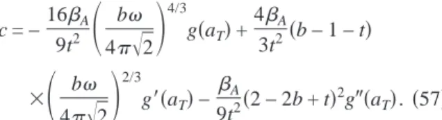
In addition to the␦-function-like spike at melting for spe-cific heat experiments, the experiments also show spespe-cific heat jump. The theory allows us to quantitatively estimate it. The specific heat contribution due to the vortex matter is C = −T⳵2_/_⳵_T2_G_{共T,H兲. The normalized specific heat is} de-fined as c = C C_mf, 共56兲 where Cmf= Hc2 2 T / 4␲␬2␤ATc 2

is the mean-field specific heat of the solid. Substituting the definition of the scaled free energy, Eq.(15), and scaled temperature, Eq. (13), we obtain

c = −16␤A 9t2

冉

b␻ 4␲

冑

2

冊

4/3 g共a_T兲 +4␤A 3t2共b − 1 − t兲 ⫻

冉

b␻ 4␲

冑

2

冊

2/3 g

⬘

共aT兲 − ␤A 9t2共2 − 2b + t兲 2_g

_⬙

_共a T兲. 共57兲

Using our expressions for the energy of the liquid and solid we obtain the following specific heat jump at melting:

TABLE II. Parameters of high Tcsuperconductors deduced from the melting line.

Material T_c H_c2 Gi ␬ ␥ Reference YBCO7−␦ 93.1 167.5 1.9⫻10−4 48.5 7.76 2 YBCO₇₋_␦ 92.6 190 2⫻10−4 ₅₀ _8.3 ₄₀ YBCO7 88.2 175.9 7.0⫻10−5 50 4 6 DyBCO_6.7 90.1 163 3.2⫻10−5 _33.77 _5.3 ₈ 共K,Ba兲BiO3 31 26 5.3⫻10−5 107 1 41

(11)

⌬c = 0.0075

冉

2 − 2b + t t

冊

2 − 0.20N_Gi1/3共b − 1 − t兲

冉

b t2

冊

2/3 . 共58兲 Using the parameters of YBCO7−␦ obtained by fitting the melting line, Table II, we compare Eq.(58) with the experi-mental result of Ref.2 in Fig. 2 of Ref. 18(right inset). Note that error bars are very large and also that disorder might be important,51_{so that the agreement of the theoretical and} ex-perimental result of specific jump is not good as that of the magnetization jump.

V. HIGHER-LANDAU-LEVEL CONTRIBUTIONS: EFFECTIVE LLL MODEL

A. Where is the LLL approximation really valid? Contributions of HLL are important phenomenologically in two regions of the phase diagram. The first is at a tem-perature above the mean-field critical temtem-perature Tc共H兲

in-side the liquid phase. The second is far below the melting point deep inside the solid phase.

Naively in the solid phase, when “distance from the mean-field transition line” is smaller than the “inter-Landau-level gap,” 1 − t − b⬍2b, one expects that higher-Landau-level harmonics can be neglected. A more careful examina-tion shows that a weaker condiexamina-tion 1 − t − b⬍12b should be used for a validity test of the LLL approximation44_to calcu-late the mean-field LLL contributions in a vortex solid. An additional factor of 6 comes from the hexagonal symmetry of the lattice since contributions of higher Landau levels, the first to the fifth HLL, do not appear in the perturbative cal-culation of the mean-field solution for a vortex solid. In the liquid state the question has been studied by Lawrie62_using the Hartree-Fock(Gaussian) approximation. The result was that the region of validity is limited, but quite wide; see Fig. 1.

In this section we will incorporate the leading HLL cor-rection using the Gaussian approximation and then compare the theoretical results with experimental magnetization curves.

B. Gaussian approximation in the liquid phase The free energy density beyond the LLL approximation is

G = − ␻Hc2 2 2␲␬2Nvol log

冕

D␺D␺¯ exp

冉

− 1 ␻

冕

d 3_x1 2兩⳵z␺兩 2 − ah兩␺兩2+ 1 2兩␺兩 4

冊

_, _共59兲

where N_voldenotes volume. In the framework of the Gauss-ian(Hartree-Fock) approximation the free energy is divided into an optimized quadratic part K and a “small” part V. Then K is chosen in such a way that the Gaussian energy is minimal.62 _{The Gaussian energy is a rigorous lower bound} on energy. Due to the translational symmetry of the vortex liquid, an arbitrary U(1)-symmetric quadratic part K has only one variational parameter␧:

K = 1 ␻

冕

d 3_x

冉

1 2共兩D␺兩 2_{− b}_兩_␺_兩2_{兲 +}1 2兩⳵z␺兩 2₊_␧兩_␺_兩2

冊

_. 共60兲 The small perturbation is therefore

V =1

␻

冕

d3x

冋

共− ah−␧兲兩␺兩2+

1 2兩␺兩

4

册

_. _共61兲 The Gaussian energy consists of two parts. The first is the “Tr log” term

− ␻Hc2 2

2␲␬2_vollog

冋

冕

D␺exp共− K兲

册

=

⬘

+␻共u

⬘

兲2+ u. 共67兲 Thus the temperature Tc and vacuum energy will be

(12)

renor-malized. The first two terms in the free energy are divergent and linear in the fluctuation temperature ␻; they will not contribute to any physical quantities like magnetization and specific heat. Minimizing the energy, Eq. (67), we get the gap equation

␧ = − ah

r_{+ 2}_␻_u

_⬘

_. _共68兲

Superscript r will be dropped later on. The function u共␧,b兲 can be written in the form

u共␧,b兲 = 1

冑

2␲b 3/2_v

冉

␧ b

冊

, 共69兲 where v共x兲 =

兺

n=0 ⬁

冋

= 1 / 20. One observes that, apart from the fields smaller than HLLL⬇0.1 T for YBCO, the experimentally observed

melt-ing line and its neighborhood are well within the range of applicability of this approximation as shown in Fig. 1.

The effective LLL energy (we will use unit of energy density H_c22 / 2␲␬2in this subsection) functional is defined by

gef f关␺0兴 = − ␻ Nvol log

冕

兿

i=1 ⬁ D␺iD␺i *_exp_{兵− f关}_␺ 0,␺0 *_,_␺ i,␺i *_,_兴其, 共72兲 where␺0 is the LLL N = 0 component field and the rest are denoted by ␺_i. Expanding the functional up to the fourth order in␺0 and to the second order in⳵zone obtains

gef f关␺0兴 = ⌬g + ⌬t 2 兩␺0兩 2₊_␻_f LLL关␺0兴, fLLL关␺0兴 = 1 ␻

冋

1 2兩⳵z␺0兩 2_{− a} h兩␺0兩2+ 1 2兩␺0兩 4

册

_. _共73兲 The direct(no␺0 dependence) renormalization of energy is

⌬g = − ␻ Nvol log

冕

兿

i=1 ⬁ D␺iD␺i *_exp_{兵− f} HLL关␺i兴其, 共74兲

where the HLL energy is

f_HLL= 1 ␻

冋

1 2兩⳵z␺HLL兩 2_{− a} h兩␺HLL兩2+ 1 2兩␺HLL兩 4

册

_, _共75兲 where␺HLL=兺i=1⬁ ␺i. To calculate⌬g, we divide the fHLLinto

K_HLL= 1 ␻

冉

1 2共兩D␺兩 2_{− b}_兩_␺_兩2_{兲 +}1 2兩⳵z␺兩 2₊_␧兩_␺_兩2

冊

_共76兲 plus fHLL− KHLL. Taking␧ as the solution of the gap equation

(68), one finds that⌬g takes the form

⌬g = gGauss− gLLL+ 2具兩␺0兩2典共具兩␺0兩2典 − 具兩␺兩2典兲, gLLL= − ␻ Nvollog

冕

D␺0D␺0 * exp兵− fLLL关␺0兴其. 共77兲 Here gGauss is the effective free energy of the full GL

ob-tained in the first subsection of the current section, Eq.(67), and具兩␺兩2典 is likewise the expectation value of 兩␺兩2in the full GL. The quantity g_LLL is the effective free energy calculated with variational parameter ␧ and 具兩␺0兩2典 is the expectation value in the LLL GL. The consistency(or matching) require-ment is gef f= − ␻ Nvol log

冕

D␺0D␺¯0exp

再

− 1 ␻gef f关␺0兴

冎

. 共78兲 This condition determines the value of⌬t:

⌬t = 4共具兩␺兩2_{典 − 具兩}_␺ 0兩2典兲 = 4␻关u

⬘

共␧,b兲兴 − 4具兩␺0兩2典 = 4␻

_冑

1 2␲b 1/2

冋

_v

_⬘

冉

␧ b

冊

− 1 2

冑

b ␧

册

. 共79兲

For Y BCO, the correction⌬t is small. The effective LLL GL approach achieves a simplification by starting from the LLL effective model with T_cand other parameters renormalized to account for the contribution of the HLL modes. This is what we assumed in Secs. III and IV. In particular, this approach is very precise if we calculate the properties along the melting line. For example, the magnetization jump is mostly due to the fluctuation of the LLL modes, and the background effec-tive energy ⌬g will not contribute anything since it is the same on both sides of the melting line.

D. HLL contribution to the magnetization

Generally when␬is quite large and magnetization can be approximated by

M = − ⳵

⳵HG共T,H兲. 共80兲

The HLL correction will be calculated as follows. We nu-merically solve the gap equation(68) from which G共T,H兲 can be obtained. Then Eq.(80) is used to calculate the mag-netization of the full GL model in the Gaussian