使用者輔助的網格參數化

全文

(1)國立交通大學資訊工程系碩士論文. 使用者輔助的網格參數化. User-Assisted Parameterization of Polygonal Meshes. 研究生：戴文政指導教授：莊榮宏. 博士. 中華民國九十三年七月.

(2) 使用者輔助的網格參數化 User-Assisted Parameterization of Polygonal Meshes. 研究生 : 戴文政. Student : Wen-Zheng Dai. 指導教授 : 莊榮宏博士. Advisor : Dr. Jung-Hong Chuang. 國立交通大學資訊工程學系碩士論文 A Thesis Submitted to Institute of Computer Science and Information Engineering College of Electrical Engineering and Computer Science National Chiao Tung University in Partial Fulfillment of the Requirements for the Degree of Master in Computer Science and Information Engineering July 2004 Hsinchu, Taiwan, Republic of China. 中華民國九十三年七月.

(3) 使用者輔助的網格參數化研究生 : 戴文政. 指導教授 : 莊榮宏博士. 國立交通大學資訊工程學系. 摘. 要. 在三維電腦繪圖裡網格參數化一直以來都是很基本且重要的問題，它可被運用於許多的電腦繪圖領域，如貼圖(texturing mapping)、貼圖合成(texture synthesis)、互動式三維描繪(interactive 3D painting)、網格重建 (remeshing)、多解析度分析和網格壓縮(multi-resolution analysis)。之前的參數化演算法都是自動且全域性的達到最小失真參數化，但是這種最小失真的參數化不一定適合於每個電腦繪圖領域，如網格重建。在這篇論文裡，我們提出一個可讓使用者調整局部的參數化的架構來改善網格重建的品質。. i.

(4) User-Assisted Parameterization of Polygonal Meshes. Student : Wen-Zheng Dai. Advisor : Dr. Jung-Hong Chuang. Department of Computer Science and Information Engineering National Chiao Tung University. ABSTRACT Surface parameterization is a fundamental problem in computer graphics. It is very useful in many applications such as texture mapping, texture synthesis, interactive 3D painting, re-meshing, multi-resolution analysis, and mesh compression. However, previous parameterization methods automatically and globally balanced the distortion of area or angle in the embedding functions. Such a parameterization may have low distortions but might not be suitable for some applications, such as remeshing. In this thesis, we present a framework that allows users to locally adjust the parameterization intending to improve the perceptual quality of remeshing.. ii.

(5) Acknowledgement First, I would like to thank my advisor Jung-Hong Chuang for his guidance on research and encouragement in past two years. He led me to the field of computer graphics and mesh parameterization. I would like to thank Dan-Chi Ho for his help and advice on my thesis work. His collaboration in the work of user-assisted parameterization is highly appreciated. Pursuing master degree is not fascinating without talented and friendly people. Thanks to all my colleagues in CGGM lab, holmes, ksl, imm, malkhut, Rey, mousep, rekan, wylee, and chihchun from bottom of my heart. Thanks to all of them for their help and all the excitement. Last but not least, I would like to thank my mother for her greatest love and financial support. Without her, all above wonderful experience would not happen.. iii.

(6) Contents Nomenclature List of Figures List of Tables 1. 2. Introduction…………………………………………………………1 1.1. Problem Description…………………………..………………………….....1. 1.2. Contributions……………………………..…………………………………2. 1.3. Motivating Applications……………………………..………………….......2. 1.4. Overview of Thesis……………………………………………….………...3. Background and Related work……………………………………..4 2.1. 2.1.1. General setup and notation…………………………………………….4. 2.1.2. Spring model...………………………………………………………...6. 2.1.3. Convex combination maps………………………………………….....7. 2.1.4. First fundamental form…………………………………………….......8. 2.2. 3. Theoretic background of global parameterization…………………………..4. Related work…………………………………………………………….....11. 2.2.1. Parameterization……………………………………………………...11. 2.2.2. Applications of parameterization…………………………………….13. User-Assisted Parameterization of Polygonal Meshes…………..15 3.1. Overview…………………………………………………………………..15. 3.2. Topological surgery………………………………………………………..17 iv.

(7) 4. 5. 3.3. Initial parameterization……………………………………………………22. 3.4. Weighted L2 metric………...………………………………………………22. 3.5. Re-parameterization via the iterative global optimization……...…………24. 3.6. Re-parameterization via the spring model………………………………....27. Applications and Performance Analysis………………………….28 4.1. Applications……………………………………………………………….28. 4.2. Performance analysis……………………………………………………...36. Summary and Future work……………………………………….40 5.1. Summary…………………………………………………………………..40. 5.2. Future work………………………………………………………………..41. Bibliography……………………………………………………………42. v.

(8) Nomenclature T : Triangulation t : Triangle of T S : Triangulation in parameter domain s : Triangle of S V(T) : Vertex set of T E(T) : Edge set of T F(T) : Face set of T. VI : Interior vertices VB : Boundary vertices Π S : Parameter domain (also called “fundamental domain” or “parameter space” ) Ω : Differentiable surface. ΩT : Surface of triangulation T Ω *T : Closed-surface Ω T' : Opened-surface (topological disk). φ : Parameterization. vi.

(9) ψ : Embedding; inverse of parameterization φ J. : Jacobian matrix. ρ : Cut. ρ ' : Opened cut D : Unit square parameter domain C : Unit circle parameter domain. {R f } : Parameter-fixed regions. {R a } : Parameter-assisted regions {Ru } : Unselected regions. L2w : adaptive weighted L2 metric. vii.

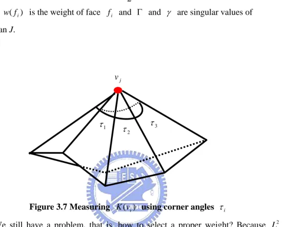
(10) List of Figures 2.1 Relations of parameterization φ and embedding ψ ………..……………..…...5 2.2 Replace each edge of the surface mesh with a spring……………………………6 2.3 Singular values of f represent the largest and smallest local stretch……………10 3.1 Parameter-adjusted regions {Ra } and parameter-fixed regions {R f } . (a) Original model with cut. (b) Paint {Ra } (green color) and {R f } (yellow color) on model by users . (c) Parameterization before adjusting. (d) Parameterization after adjusting………………………………………………………………………...15 3.2 Procedure of parametering closed-surface……………………………………...17 3.3 Slice closed-mesh open along cut………………………………………………18 3.4 Parameterization and texture mapping of two different cuts for the bunny ear...20 3.5 Parameterization and remeshing with (a and b) or without (c and d) topological boundary constraints……………………………………………………………21 3.6 Relations between sampling ratio in parameter space and Γ ⋅ γ ……………….22 3.7 Measuring K (vi ) using corner angles τ i …………………………………….23 3.8 Local minimization in parameter space…………………………………………24 4.1 Creation of initial parameterization. (a) original mesh with cut (12948 triangles; genus 0). (b) initial paramterization……………..……………………………...29 4.2 User-assisted parameterization. (a) green color region are {Ra } painted by users. (b) before diffusing virtual distortions. (c) after diffusing virtual distortions……………………………………………………………………….30 4.3 Remesing results of fandisk. (a) remeshing of initial parameterization. (4802 viii.

(11) triangles) (b) remeshing of user-assisted parameterization. (4802 triangles) (c) wireframe of (a). (d) wireframe of (b)…………………………………………..30 4.4 Comparisons of initial parameterization (left column) and user-assisted parameterization (right column) on the Fandisk model with different sampling resolutions………………………………………………………………………31 4.5. Remesing results of cube. (a) remeshing using the initial parameterization. (1922 triangles) (b) remeshing using the user-assisted parameterization. (1922 triangles) (c) wireframe of (a). (d) wireframe of (b)………………....................32. 4.6 Comparisons of initial parameterization (left column) and user-assisted parameterization (right column) on the Cube model with different sampling resolutions…………………………………………………………………..…33 4.7 Remesing results of venus. (a) original model. (b) original model with painting. (c) remeshing results using the initial parameterization. (d) remeshing results using the user-assisted parameterization………………………………………34 4.8 Remesing results of isis. (a) original model. (b) original model with painting. (c) remeshing results using the initial parameterization. (d) remeshing results using the user-assisted parameterization……………………………………………..35. ix.

(12) List of Tables 4.1 Statistics for cutting and initial parameterization. Cut % means cut length percent…………………………………………………………………………..37 4.2 Statistics for various stretches of initial parameterization………………………37 4.3 Statistics for user-assisted parameterization after and before re-parameterization. OS and RS mean original size and remeshing size in face……………………..38 4.4 Numbers of vertices and faces in models of different resolutions M. V and F represent respectively the vertex number and face number…………………….38 4.5 Maximum and mean hausdorff distances for remeshed Fandisk in different sampling resolutions…………………………………………………………….38 4.6 Maximum and mean hausdorff distances for remeshed cube in different sampling resolutions...…………………………………………………………………….39. x.

(13) Chapter 1 Introduction In this chapter, we present the problem statement, our contribution, motivated applications, and finally the organization of the thesis.. 1.1 Problem Description Parameterization denotes the task of finding a two dimensional map for a surface in a higher dimension. Perfect parameterization (isometric parameterization) demands the bijective mapping from surface to parameter space that preserves the metric structure of the surface, i.e. respect area and angles of shapes. Unfortunately, in general such an angle and area preserving parameterization does not exist except for the developable surfaces. Thus most current research of parameterization tends to minimize the global energy [3, 4, 17] or distortions (angle or area) [8, 20, 25] over the surface during the parameterization. Since parameterization distortions are minimized globally, some applications may find under-sampling in the areas of geometric or semantic features, such as sharp edges or high frequency color. Parameterizations that take signal variation into account was presented previously. However, it cannot satisfactorily avoid the problem. Since perceptual importance is ultimately determined by a human observer, we argue that human assistance in the parameterization process is a natural way to solve the problem. In this thesis, we provide a novel method that allows users to locally control the parameterization for improving the sampling quality.. 1.

(14) 1.2 Contributions This thesis describes a novel, user interactive framework for mesh parameterization. Along the way to achieve this goal, we present the following contributions:. z A weighted L2 metric L2w to increase the sampling ratio of selected regions in parameter space z A simple iterative global optimization algorithm to re-parameterize the triangle mesh with facet parameter constraints z A alternative approach to re-parameterize the triangle mesh via the spring model without facet parameter constraints z An interface for user-assisted parameterization. 1.3 Motivated Applications In this section, we briefly introduce several applications to motivate our research. The following are some examples of them.. Texture Mapping Texture mapping is at the heart of modern computer graphics rendering techniques. Texturing the mesh will be as simple as pasting a picture on to the parameter space, and mapping each triangle of the original mesh with the part of the picture present within the associated triangle in the parameter space.. Remeshing in Geometry Images Geometric models are always represented as irregular meshes. By mapping them to the plane, one can resample the geometric surface with uniform sampling [6] or non-uniform sampling [1]. In order to improve the efficiency for hardware rendering, it is better to use the regular sampling pattern. Since our algorithm adjusts the 2.

(15) important regions in parameter space to get better remeshing quality and keep the uniform sampling pattern in parameter space, it benefits to the construction of geometry image.. Surface Compression By using parameterization, geometric models can be remeshed in geometry image, then be compressed by any image coders [30]. Since our algorithm keep the regular sampling points in real important regions, it has lower compression ratio compared to other parameterization algorithms.. Painting System A 3D painting system [10] makes it possible to enhance the visual appearance of a 3D model by interactively adding details to it, such as colors, normals, reflections etc. If the discretization of the surface is fine enough, it is possible to directly paint its vertices. However, in most cases, the desired precision for the colors is finer than the geometric details of the model. Assuming that the surface to be painted is provided with a parameterization, it is convenient to use texture mapping to store colors in the parameter space, and virtually glue the texture image to the model. Because our method provides users to control the local parameterization quality (distortions), it is very suitable for painting systems.. 1.4 Overview of Thesis In the next chapter, we discuss the fundamental background of parameterizations and review some previous work in mesh parameterization and its applications. In chapter 3, the method for user-assisted parameterization is explained in details. Chapter 4 demonstrates some applications and analyzes the performance of the method. Chapter 5 summarizes the method presented and mentions some research directions.. 3.

(16) Chapter 2 Background and Related work In this chapter, we discuss fundamental background and previous methods for parameterizing meshes onto the 2D plane. First, we review some fundamental theory of global parameterization used in our research. Next, we introduce previous work of paramterization and its application.. 2.1 Theoretic background of global parameterization Parameterization is a mapping from two dimensions to higher dimensions. To measure the distortions of the mapping, there are many energy models (e.g. harmonic energy) or metrics (e.g. Cauchy-Riemann equation) to estimate the distortions after the mapping process. For building solid theoretic foundation of our research, in this section, we only introduce energy models and metrics directly related to our research.. 2.1.1 General setup and notation. Before we review the fundamental theory, we first introduce some basic concepts and symbols to help us introduce the fundamental theory.. 4.

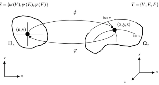
(17) S = {ψ (V ),ψ ( E ),ψ ( F )}. T = {V , E , F }. φ iso-v. (x,y,z) (u,v) iso-u. ΠS. ΩT. ψ. y. v. x u z. Figure 2.1 Relations of parameterization φ and embedding ψ . See Figure 2.1, we call Ω T ∈ R 3 the surface of the triangulation T and further let. V = V (T ) denote the set of vertices, E = E (T ) the set of edges, and F = F (T ) the set of faces in T. If Ω T has a boundary we distinguish between the disjoint sets of interior and boundary vertices VI and V B . Two distinct vertices v, w ∈ V are neighbors if they are the end points of an edge e = [v, w] ∈ E and for v ∈ V we let N v = {w ∈ V : [v, w] ∈ E} be the set of neighbors of v. In general parameterization φ of a triangulation T over a parameter domain Π T ∈ R 2 is a homeomorphism between this domain and the surface of T ,. φ : Π T → ΩT From differential geometry [31], we know that such a homeomorphism and the inverse parameterization (also called as “surface embedding”) ψ = φ −1 exist if and only if Π T and Ω T are topologically equivalent, i.e. Π T is a 2-manifold with the same number of boundaries and handles as Ω T . The number of handles is also called the genus of a manifold. For example, a sphere has genus zero and the genus of a torus is one, etc. If Ω T and Π T are not topologically equivalent, we should do some topological operations to change topology of Ω T to be equivalent to Π T . In this thesis, we also cover this problem and we provide a method for doing this.. 5.

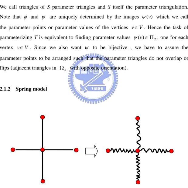
(18) For triangulations the most natural class of parameterizations are piecewise linear functions. Due to the piecewise linearity, ψ induces a triangulation. S = {ψ (t ) : t ∈ T } , with ψ (Ω T ) = Π T which is equivalent to T in the sense that vertices, edges and triangles of S and T naturally correspond to each other,. ψ (V (T )) = V ( S ) , ψ ( E (T )) = E ( S ) , ψ (T ) = S , and. φ (V ( S )) = V (T ) ,. φ ( E ( S )) = E (T ) ,. φ (S ) = T .. We call triangles of S parameter triangles and S itself the parameter triangulation. Note that φ and ψ are uniquely determined by the images ψ (v) which we call the parameter points or parameter values of the vertices v ∈ V . Hence the task of parameterizing T is equivalent to finding parameter values ψ (v) ∈ Π T , one for each vertex v ∈ V . Since we also want ψ to be bijective , we have to assure the parameter points to be arranged such that the parameter triangles do not overlap or flips (adjacent triangles in Ω S with opposite orientation).. 2.1.2 Spring model. Figure 2.2: Replace each edge of the surface mesh with a spring.. The first class of linear parameterization methods is motivated by a physical model [9]. By replacing each edge of the triangulation with a spring, we obtain a network of 6.

(19) springs with joints (Figure 2.2). The total energy of this system is. E S (ψ ) =. 1 1 Dvw ψ (v) − ψ ( w) ∑ 2 [ v , w]∈E 2. 2. (2.1). with certain (strictly positive) spring constants Dvw = Dwv , the additional factor 1/2 occurring because each edge is summed up twice. The partial derivative of ES with respect to ψ (v) is ∂E S (ψ ) = ∑ Dvw (ψ (v) − ψ ( w)) ∂ψ (v) w∈N v. (2.2). and minimizing (2.1) subject to the boundary conditions of ψ (v) being fixed for all v ∈ VB is equivalent to solving the linear system of equations. ψ (v) ∑ Dvw = w∈N v. ∑D. w∈N v. ψ ( w) ,. v ∈ VI. vw. (2.3). If we separate the interior and the boundary vertices in the sum on the right side of (2.3), we can rewrite this linear system as. ψ (v) ∑ Dvw − w∈N v. ∑. w∈N v ∩ w∈VI. Dvwψ ( w) =. ∑D. ψ ( w) ,. vw w∈N v ∩ w∈VB. v ∈ VI. (2.4). or, more compact, as the matrix equation Ax = b. (2.5). where x = (ψ (v)) v∈VI is the column vector of unknowns, b is the column vector. whose elements are the right hand sides of (2.4), and the symmetric matrix A = (avw ) v , w∈VI has dimension VI × V I. a vw. and elements. ⎧∑ u∈N v Duv , w = v, ⎪ = ⎨ − Dvw , w ∈ Nv ⎪ 0, otherwise. ⎩. (2.6). 2.1.3 Convex combination maps. Another linear parameterization method was introduced by Floater [5]. As in the previous sections, the first step of that method is to specify the parameter points ψ (v) of the boundary vertices v ∈ VB . Then, for each interior vertex v ∈ VI a set of strictly positive convex weights λvw , w ∈ N v with 7.

(20) ∑λ. w∈N v. =1. vw. (2.7). is chosen and the remaining ψ (v) , v ∈ VI are determined by solving the linear system of equations. ψ (v ) =. ∑λ. w∈N v. ψ ( w) ,. v ∈ VI. vw. (2.8). Therefore, every interior parameter point is a convex combination of its neighbors. Like in Section 3.1.2, by separating interior and boundary vertices, (2.8) can be rewritten as. ψ (v ) −. ∑. w∈N v ∩ w∈VI. λvwψ ( w) =. ∑λ. ψ ( w) ,. vw w∈N v ∩ w∈VB. v ∈ VI. (2.9). and further as Bx = c. (2.10). where x = (ψ (v)) v∈VI is again the column vector of unknowns, c is the column vector whose elements are the right hand sides of (2.9), and the VI × VI. matrix. B = (bvw ) v , w∈VI has elements. bvw. w = v, ⎧ 1, ⎪ = ⎨− λvw , w ∈ N v , ⎪ 0, otherwise. ⎩. (2.11). Note that in general λvw ≠ λ wv and therefore B is usually not symmetric in contrast to A in (2.5). Comparing (2.11) with (2.6), the convex combination maps can also be validated by the spring model because λvw can be rewrote with Dvw given by. λvw =. Dvw , ∑w∈N Dvw. v ∈ VI ,. w ∈ Nv. (2.12). v. 2.1.4 First fundamental form. We have introduced two fundamental linear models of parameterizing the triangulated. 8.

(21) mesh Ω T . In this section, we introduce more complicated metrics of parametering Ω T based on the first fundamental form from differential geometry [31].. Given a differentiable surface Ω and its parameterization φ . We can regard parameterization φ as a mapping from R 2 to R 3 by. φ (u, v) = [ x(u, v), y (u, v), z (u, v)]. (2.13). Consider the first fundamental form of Ω : dl 2 = E (u, v)du 2 + 2 F (u, v)dudv + G (u, v)dv 2. (2.14). and arrange the coefficients in a symmetric matrix. ⎡E F ⎤ I =⎢ ⎥ ⎣F G⎦. (2.15). we have. ⎛ du ⎞ dl 2 = (du dv )I ⎜⎜ ⎟⎟ ⎝ dv ⎠ ∂φ ∂φ ∂φ ∂φ ∂φ ∂φ ⋅ ⋅ ⋅ . I is called the metric tensor and its where E = , F = , and E = ∂u ∂u ∂u ∂v ∂v ∂v eigenvalues denoted by Γ 2 and γ 2 . Then we decompose I as I = JTJ. and. J = [∂φ / ∂u, ∂φ / ∂v]. (2.16). where J is the Jacobian matrix and Γ and γ are singular values of J. Since J can be seen as local affine mapping from R 2 to R 3 by ⎛ p⎞ q = ( J ο )⎜⎜ ⎟⎟ , ⎝1⎠. q, ο ∈ R 3 ,. p ∈ R2. (2.17). where ο is the original point for completing the affine mapping, it is convenient to use Γ and γ for describing the lengths and angles of vectors in R 2 after being mapped by φ . In other words, the singular values Γ and γ represent the largest and smallest length obtained when mapping unit-length vectors from R 2 to R 3 , i.e. the largest and smallest local “stretch”.. 9.

(22) p1. q3 q1. γ Γ. linear map f p2. p3. parameter domain. ΠS. q2. triangulated surface Ω T. Figure 2.3 Singular values of f represent the largest and smallest local stretch. Now we turn our focus on triangulated surface Ω T . Because triangulated surface Ω T is piecewise linear, φ can be seen as the piecewise linear map f (Figure 2.3).. From above discussion, we can imagine that f of Ω T is corresponding to J of Ω . Since the common way to represent f is the barycentric mapping B(p) B ( p ) = (< p, p 2 , p3 > q1 + < p, p3 , p1 > q 2 + < p, p1 , p 2 > q3 ) / < p1 , p 2 , p3 >. (2.18). where <a, b, c> denotes the area of triangle abc, p ∈ R 2 , q ∈ R 3 , we can discretize J by ⎡∂B / ∂u ⎤ ⎡∂x / ∂u ∂y / ∂u ∂z / ∂u ⎤ J =⎢ =⎢ ⎥ ⎥ ⎣ ∂B / ∂v ⎦ ⎣ ∂x / ∂v ∂y / ∂v ∂z / ∂v ⎦ t. t. and ∂B / ∂u = Bu = (q1 (v 2 − v3 ) + q 2 (v3 − v1 ) + q3 (v1 − v 2 ) /(2 A) ∂B / ∂v = Bv = (q1 (u 3 − u 2 ) + q 2 (u1 − u 3 ) + q3 (u 2 − u1 ) /( 2 A). where A =< p1 , p 2 , p3 >= ((u 2 − u1 )(v3 − v1 ) − (u 3 − u1 )(v 2 − v1 )) / 2 . Thus the Jacobian matrix of Ω T is ⎡ x1 1 ⎢ JT = y1 2A ⎢ ⎢⎣ z1. x2 y2 z2. x3 ⎤ ⎡(v 2 − v3 ) (u 3 − u 2 )⎤ y 3 ⎥⎥ ⎢⎢ (v3 − v1 ) (u1 − u 3 ) ⎥⎥ z 3 ⎥⎦ ⎢⎣ (v1 − v 2 ) (u 2 − u1 ) ⎥⎦. and the larger and smaller singular values of J T are given respectively by. 10. (2.19).

(23) Γ = 1 / 2⎛⎜ (a + c ) + ⎝. (a − c )2 + 4b 2 ⎞⎟ ⎠. max singular value of J T. (2.20). γ = 1 / 2⎛⎜ (a + c ) −. (a − c )2 + 4b 2 ⎞⎟. min singular value of J T. (2.21). ⎝. ⎠. where a = Bu ⋅ Bu , b = Bu ⋅ Bv , and c = Bv ⋅ Bv . Based on above deduction, many researchers proposed various stretch metrics by the versatile Γ and γ . For example, Sander et al. [20] define an L2 distortion measure by taking the root-mean-square of Γ and γ , and define L∞ by take the largest singular value Γ as follows : Γ2 + γ 2 2. L2 =. L∞ = Γ ,. (2.22) (2.23). Hormann et al. [8] define their deformation metric as Ld =. Γ. γ. +. γ Γ. ,. (2.24). Sorkine et al. [26] define their geometric distortion as L g = max{Γ,1 / γ } ,. (2.25). Khodakovsky et al. [11] define area distortion as Larea = Γ ⋅ γ ,. (2.26). and anisotropic distortion as Langle =. Γ. γ. (2.27). 2.2 Related work 2.2.1 Parameterization Over the last years, a lot of research has been done in the area of surface parameterization. Besides, methods that optimize the parameterization for a given surface signal like Sander et al.[19], most approaches aim at minimizing a metric distortion. In the context of parameterization, harmonic maps were first used by Eck et 11.

(24) al.[4]. To compute harmonic maps, Eck et al. derive appropriate weights for a system of edge springs which can be efficiently solved. However, the texture coordinates for boundary vertices must be fixed a prior and harmonic maps may contain face flips (adjacent faces in texture space with opposite orientation) which violate the bijectivity of a parameterization. Based on earlier work by Tutte[27], Floater[5] proposes a different set of weights for the edge spring model that guarantees bijectivity if the texture coordinates of boundary are fixed to a convex polygon. Desbrun et al.[3] define a space of measures spanned by a discrete version of the Dirichlet energy, and a discrete authalic energy. While the authalic energy remedies local area deformations, it requires fixed boundaries and results cannot achieve the quality of methods targeted at global length preservation such as Sander et al. [20]. In Hormann and Greiner[8], mostly isometric parameterization are introduced that minimize a non-linear energy. Mostly isometric parameterizations do not require boundary texture coordinates to be fixed and avoid face flips. Furthermore, mostly isometric parameterizations approximate mathematically well studied continuous conformal maps, i.e. maps that perfectly preserve angles. Another approach to minimize angular distortion is proposed by Sheffer and Sturler[25]. They introduce a angle based flattening method to flatten a mesh to a planar plane so that it minimizes the relative distortion of the planar angles with respect to their counterparts in the three-dimensional space. Though the minimization problem is linear in the relative distortion of angles, it becomes non-linear as a number of constraints (some of which are non-linar) have to be taken into account to generate the validity of the solution. Levy et al.[15] compute quasi-conformal parameterizations by measuring the violation of the Cauchy-Rieman equation in the least square sense. They also show rigorously that the quasi-conformal parameterization exists uniquely, is invariant by similarity, independent of resolution and preserves orientations. Using a standard numerical conjugate gradient solver they are able to compute least squares approximations to continuous conformal maps very efficiently without requiring fixed boundary texture coordinates. However, in seldom cases triangle flips may occur. In addition, some methods exist which compute parameterizations over a 12.

(25) non-planar domain. In Lee et al.[12], a mesh simplification is used to parameterize a surface over a base mesh. A similar approach is taken by Khodakovsky et al.[11] but with emphasis on globally smooth derivatives. Besides angle preserving methods, only a few approaches explicitly optimize global area or global length distortions: Maillot et al.[17] minimize an edge length distortion, but cannot guarantee the absence of face flips. The authors also propose an area preserving energy and combine both energies in a convex combination. Sander et al.[20] minimize the average or maximal singular value of the Jacobian to prevent undersampling of the surface. However, their metric cannot penalize the anisotropic stretching- triangles whose stretch in one direction is significantly higher than in the other direction. As a result of anisotropic stretching, parameterization of [20] has the parametric cracks problem. Yoshizawa et al. [28] improve parametric cracks with adaptively adjusting the spring constants by L2 metric.. 2.2.2 Applications of parametrization Remeshing. Alliez et al.[1] proposed an interative sampling technique. A mesh is decomposed into a set of maps by parameterization and inserted in a pipeline of signal processing algorithms. The output of this pipeline is density map, interatively resampled using an error diffusion technique commonly used for gray level image halftoing.. Geometry video. Briceno et al.[2] present geometry videos based on geometry image to represent animation. Geometry videos resample and reorganize the geometry information, in such a way, that it becomes very compressible. They provide a unified and intuitive method for level-of-detail control, both in terms of mesh resolution (by scaling the two spatial dimensions) and of frame rate (by scaling the temporal dimension). Since geometry videos have a very uniform and regular structure. Their source and computational requirements can be calculated exactly, hence making them also 13.

(26) suitable for applications requiring level of service guarantees.. 3D Painting system. Igrashi et al.[10] present a method for dynamically generating an efficient texture bitmap and its associated UV-mapping in an interactive texture painting system for 3D models. They proposed an adaptive and local parameterization mechanism where system dynamically creates a tailored UV-mapping for newly painted polygons during interactive painting process. This eliminates the distortion of brush strokes, and the resulting texture bitmap is more compact because the system allocates texture space only for the painted polygons. In addition, this dynamic texture allocation allows the user to paint smoothly at any zoom level.. Constrained texture mapping. Levy et al.[14] introduce constrained texturing mapping by parameterizing polygonal meshes with minimum deformation between source textures. They enable users to interactively define and edit a set of constraints. Each user-defined constraint consists of a relation linking a 3D point picked on the surface and 2D point of the texture. Moreover, the non-deformation criterion introduced here can act as an extrapolator, thus making it unnecessary to constrain the border of the surface, in contrast with classic methods. To minimize the criterion, a conjugate gradient algorithm is combined with a compressed representation of sparse matrices, making it possible to achieve a fast convergence.. Mesh editing. Levy et al.[16] introduce an idea in editing the mesh on parameter domain. They proposed an objective function of squared curvature. By minimizing this objective function, they extrapolate mesh shape beyond the existing border. In addition, the parameter space provides the user with a new means of controlling the shape of the surface.. 14.

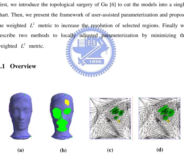
(27) Chapter 3 User-Assisted Parameterization of Polygonal Meshes In this chapter, we describe the user-assisted parameterization of polygonal meshes. First, we introduce the topological surgery of Gu [6] to cut the models into a single chart. Then, we present the framework of user-assisted parameterization and propose the weighted L2 metric to increase the resolution of selected regions. Finally we describe two methods to locally adjusted parameterization by minimizing the weighted L2 metric.. 3.1 Overview. (a). (c). (b). (d). Figure 3.1 Parameter-adjusted regions {R a } and parameter-fixed regions {R f } . (a) Original model with cut. (b) Paint {R a } (green color) and {R f } (yellow color) on model by users . (c) Parameterization before adjusting. (d) Parameterization after adjusting. 15.

(28) Our proposed user-assisted mesh parameterization has the following characteristics: z Topological surgery is used to automatically transform the closed-surface into an. opened-surface which is topologically equivalent to a disk;. z. Users can specify parameter-adjusted regions {Ra } , where the resolution of sampling is expected to increase in parameter space for improving the sampling quality;. z. Users can specify parameter-fixed regions {R f } , where the resolution of sampling is expected to be fixed in parameter space for keeping the sampling quality;. z Use the uniform sampling in parameter space to maintain the regular structure.. Such a uniform sampling is suitable for many applications, such as geometry image, compression etc.. To adjust the sampling resolution in parameter space, our basic idea is to increase the resolution of selected regions while decreasing the resolution of other regions. To achieve this goal, we directly multiply a weight to the L2 stretch proposed by Sander et al [20]. We call this reformulated metric the weighted L2 , denoted as L2w . Then we re-parameterize Ω T by minimizing L2w . In this thesis, we introduce two methods to re-parameterize Ω T , using the iterative global optimization and the spring model. The iterative global optimization is a non-linear process and can locally adjust the parameterization quality by increasing resolution of {Ra } and fix resolution of {R f } in parameter space. The spring model is a linear process and faster than iterative global optimization. But the drawback is that it cannot preserve facet parameter constraints for regions {R f } .. 16.

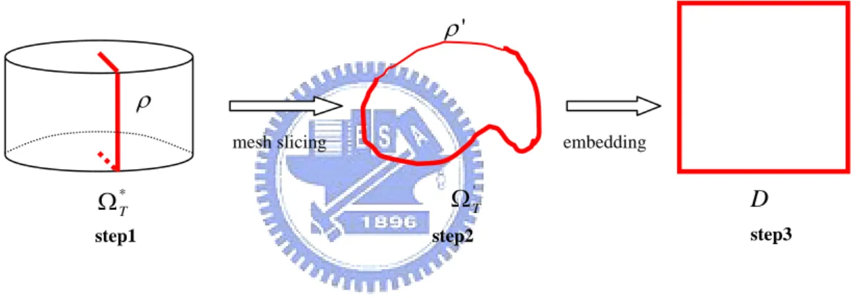
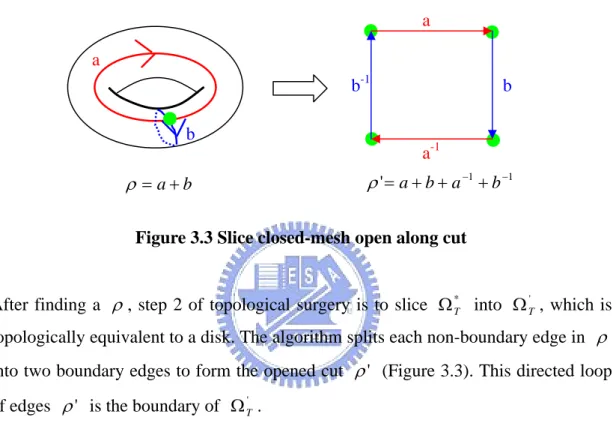
(29) Our user-assisted parameterization comprises the following steps:. 1.. Transform the closed-surface Ω *T. into an opened-surface Ω T'. by using. topological surgery, 2.. Construct a global initial parameterization for the surface mesh,. 3.. Select the regions {Ra } or {R f } on the surface mesh for increasing or preserving the sampling resolution in parameter space,. 4.. Use the iterative global optimization or the spring model to re-parameterize Ω T' .. 3.2 Topological surgery ρ' ρ mesh slicing. embedding. Ω T'. Ω *T step1. step2. D step3. Figure 3.2 Procedure of parametering closed-surface. To parameterize Ω T onto a planar domain, Ω T should be topological disk-like. Since the closed-surface Ω *T is not equivalent to a topological disk, we need to change the topology of Ω *T by splitting Ω *T into opened-surface Ω T' that is equivalent to the topological disk before embedding to unit square parameter domain D (Figure 3.2). To achieve this goal we use the topological surgery proposed in [6].. The topological surgery consists of two steps. Step 1 is finding a good cut ρ to reduce the potential distortions after mapping to D. In addition, we also wish to minimize the total length of ρ for reducing the parametric discontinuity. There are several automatic solutions to find such a ρ [6, 7, 23, 24]. In this thesis, we slightly modify Gu’s cutting algorithm [6]. The algorithm starts by finding initial cut, and then iteratively augments the cut in unit circle parameter domain C to reduce the potential 17.

(30) distortions of the embedding. The algorithm of finding initial cut is the same as that of Gu [6], but for each iteration, we use a faster parameterization proposed by Yoshizawa [28], instead of geometric stretch parameterization [20], to speed up the total process.. a a b-1 b. b. a-1. ρ ' = a + b + a −1 + b −1. ρ = a+b. Figure 3.3 Slice closed-mesh open along cut. After finding a ρ , step 2 of topological surgery is to slice Ω *T into Ω T' , which is topologically equivalent to a disk. The algorithm splits each non-boundary edge in ρ into two boundary edges to form the opened cut ρ ' (Figure 3.3). This directed loop of edges ρ ' is the boundary of Ω T' . We say that two edges in ρ ' is the boundary of Ω T' and two edges in ρ ' are mates if they result from the splitting of an edge in ρ . A vertex v with valence k in. ρ is replicated as k vertices in ρ ' . Vertices in ρ that have valence k ≠ 2 in the cut are called cut-nodes. (We still refer to these as cut-nodes when replicated in ρ ' .) A cut-path is the set of boundary edges and vertices between two ordered cut-nodes in the loop ρ ' . Each cut-path has a mate defined by mates of its edges except its edges were boundary edges in ρ . Our slicing algorithm starts to find a cut node in ρ . Then it recursively traces the path along the cut until all cut vertices and edges have been created. Note that, whenever the algorithm traces to the cut node and decides which path we should trace next, we should choose the paths clockwise to avoid path overlapping.. 18.

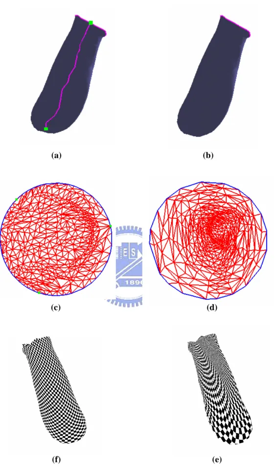
(31) Figure 3.4 demonstrate the parameterization and texture mapping results of two different cuts. Figure 3.4 (a), (b), (c), and (d) show two different cuts on the bunny ear and their respected parameterizations. Figure 3.4 (e) and (f) are images with texture mapped checkerboard. It is apparent that image of Figure 3.4 (f) reveals less angle and area stretch, which is due to the fact that the cut ρ passes through the highly curved regions of the bunny ear. Figure 3.5 shows that it is important to consider topological constraints introduced by Gu et al. [6] for remeshing to avoid parametric cracks.. 19.

(32) (a). (b). (c). (d). (f). (e). Figure 3.4 Parameterization and texture mapping of two different cuts for the bunny ear. 20.

(33) (a). (b). (c). (d). Figure 3.5 Parameterization and remeshing with (a and b) or without (c and d) topological boundary constraints. 21.

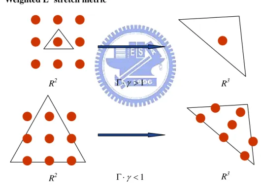
(34) 3.3. Initial parameterization. To construct a global initial parameterization of the surface, there are many solutions available [3, 4, 5, 7, 8, 9, 13, 15, 17, 19, 20, 25, 26, 28]. Although most parameterization techniques are adequate, one that aims to guarantee uniform sampling and preserve conformality structure of the input mesh is most preferable. Here, we use the method proposed by Yoshizawa et al. [28] for our initial parameterization because it has properties mentioned above. Moreover, it requires to solve a simple, sparse linear system and is usually handled in a matter of seconds using a Conjugate Gradient solver with good preconditioning.. 3.4. Weighted L2 stretch metric. R2. Γ ⋅γ > 1. R3. R2. Γ ⋅γ < 1. R3. Figure 3.6 Relations between sampling ratio in parameter space and Γ ⋅ γ. We observe that the sampling ratio in parameter space is inverse proportional to the Γ ⋅ γ (see Figure 3.7). Thus, to increase the sampling resolution of selected regions, we should decrease the Γ ⋅ γ . We indirectly minimize the Γ ⋅ γ by minimizing L2 stretch metric proposed by Sander et al [20]. Besides, in order to achieve lower value of the Γ ⋅ γ for regions in {R a } , we multiply a weight larger than one to the current L2 . The formula is given by 22.

(35) L2w ( f i ) = w ( f i ) ⋅ L2 ( f i ). (3.1). and L2 ( f i ) =. Γ2 + γ 2 2. (3.2). where w( f i ) is the weight of face f i and Γ and γ are singular values of Jacobian J.. vj. τ1. τ3. τ2. Figure 3.7 Measuring K (vi ) using corner angles τ i. We still have a problem, that is, how to select a proper weight? Because L2 metric can quantify the distortions of parameterization, we can easily use any user-specified scalar, which is larger than one, as the weight. But we want to distribute more sampling points over highly stretching regions in 3D, the constant scalar is not good enough. Therefore, we need to quantify the 3D stretching information and use this as our weight. Since the 3D stretching information is highly related to the curvature’s magnitude, we use Gaussian curvature as the weight. By Gauss-Bonnet theorem [31], we know that the Gaussian curvature of vertex v j is given by: K (v j ) = 2π − ∑ τ i. (3.3). i. where τ i is the corner angle around vertex v j (Figure 3.8). Besides, in order to get similar results for models of different resolution, we need 23.

(36) a roughly similar ratio of triangles in proportion to the size of the models. We heuristically use the log V term to compensate for the different resolution, where V is the number of vertices of the mesh. From above discussion, we finally define. our weight for each face f i as follows:. ⎧⎪log V ⋅ ∑ K (v j ) w( f i ) = ⎨ j∈ f i ⎪⎩ 1 Note that if. ∑ K (v j∈ f i. j. f i ∈ Ra f i ∉ Ra. (3.4). ) is less than one, we simply let w( f i ) = log V to avoid. parametric degenerate and negative weight.. 3.5. Re-parameterization via the iterative global optimization. d. Figure 3.8 Local minimization in parameter space. In this section, we describe the method to locally optimize the parameterization of {Ra } . The L2w increases the sampling resolution in parameter space for each face f i of {Ra } while decreasing the resolution of other regions. Besides, some regions may already have good enough resolution in parameter space. Thus we don’t want to change the resolution in such regions. For achieving this goal, our user-assisted parameterization allows users to set several facet parameter constraints in such regions to form {R f } and the iterative global optimization algorithm proposed here 24.

(37) will avoid the re-parameterization in regions of {R f } . Since our L2w metric is non-linear and we want to minimize the global L2w stretch, the optimization process can also be seen as a non-linear minimization problem. Thus we use the random descent algorithm [8, 20] to optimize our non-linear metric. Random descent algorithm employs a series of local optimization attempting to minimize distortions over the mesh. For triangulated mesh, the local minimization means adjusting the position of the vertex inside its 1-ring neighborhood (Figure 3.9) in parameter space. We perform a user specified number of iteration through all vertices in order to minimize the L2w . We now describe how each iteration is performed. We start the iteration by measuring the L2w distortion of each vertex v j , which is defined as the integrated distortions of its adjacent faces as follows L2w (v j ) =. ∑ (L. 2 w. ). ( f i ) ⋅ A( f i ) / ∑ A( f i ) 2. (3.5). where f i is an adjacent face of v j and A( f i ) is the area of f i . We then sort the vertices from the highest to the lowest distortion, and locally optimize them in that order. When optimizing each vertex, we first determine the region it belongs to. If it belongs to the parameter-fixed regions {R f } . We ignore it and pick the next vertex. Then, we pick a random search direction and set the maximum distance d, which is the distance that the vertex can move, to be the length of the longest edge adjacent to it (in parameter space). Later, we perform a binary line search minimizing distortion to place the vertex somewhere between 0 and d away from its previous position. We prevent faces from flipping (changing orientation) by setting distortion to be infinite if a triangle is flipped in the parameter space. This constraints the feasible region of the vertex to be inside the convex kernel of its neighborhood. Since the algorithm does not introduce flipped faces, it is guaranteed to produce a valid parameterization result. 25.

(38) The high-level algorithm can be summarized as follows: IterativeOptimization(Input triangle mesh Ω T ). ComputeInitStretch(); For each iteration Do SortByStretch(); For each vertex v ∈ Ω T Do If v ∉ R f OptimizeVertex(v); Endfor Until convergence. OptimizeVertex(Input vertex v) Dir <- RadomDir; R <- TrustRegionRadius; Low <- 0; High <- 1; For each iteration Do Mid <- (Low + High)/2; If Stretch(v+High*R*Dir) > Stretch(v+Low*R*Dir) High <- Mid; Else Low<-Mid; Until convergence. 26.

(39) 3.6. Re-parameterization via the spring model. If {R f } is not specified, we can directly use the spring model to locally optimize the parameterization by adjusting the spring constants Dij as follows:. Dijnew = Dijold / L2w (v j ). (3.6). Because the spring model can be solved by a linear solver, it is faster than the iterative global optimization algorithm. Moreover, in our experiment, it also has more evident remeshing results than the iterative global optimization algorithm in some cases, but the drawback is that it cannot do the re-parameterization while avoiding the entire regions in {R f } .. 27.

(40) Chapter 4 Application and performance analysis In this chapter, we demonstrate the application of our user-assisted parameterization in remeshing and show the performance analysis.. 4.1 Remeshing Geometric models often come from a variety of sources including 3D scanners, modeling software, and output from computer vision algorithms. Although these meshes capture geometry accurately, their connectivity quality is usually far from subsequent applications. For instance, irregular meshes are not appropriate for computations using Finite Elements, or for rapid, textured display on low-end computers. Uniform remeshing scheme is able to approximate an irregular mesh as a semi-regular. mesh.. When. applying. unfirom. remeshing. using. current. parameterizations, we often find it’s difficult to preserve the sharp features. Our user-assisted parameterization provides a way to solve this problem.. 28.

(41) Figure 4.1 shows the cut and an initial parameterization. Figure 4.2 demonstrates the procedure of user-assisted parameterization and the results. We directly painted the regions {Ra } over surface mesh, as shown in Figure 4.2 (a). Figure 4.2 (b)(c) are the parameterization before and after re-parameterization. The green color regions {Ra } in parameter space are corresponding to regions in 3D painted by the user and it is evident that the resolution of {Ra } becomes larger. In the Figure 4.3, Figure 4.5, Figure 4.7 and Figure 4.8, the comparison of remeshing results is shown. In addition, the remeshing quality depends on the sampling resolutions in parameter space. Thus Figure 4.4 and Figure 4.6 show the comparison of remeshing results with different sampling resolutions. Our user-assisted parameterization has better remeshing quality in lower sampling ratio than the initial parameterization.. (a). (b). Figure 4.1 Creation of initial parameterization. (a) original mesh with cut (12948 triangles; genus 0). (b) initial paramterization. 29.

(42) (a). (b). (c). Figure 4.2 User-assisted parameterization. (a) green color region are {Ra } painted by users. (b) before re-parameterization. (c) after re-parameterization.. (a). (b). (c). (d). Figure 4.3 Remesing results of fandisk. (a) remeshing using the initial parameterization. (4802 triangles) (b) remeshing using the user-assisted parameterization. (4802 triangles) (c) wireframe of (a). (d) wireframe of (b).. 30.

(43) Original : 6475 vertices, 12948 faces. M1 : 529 vertices, 968 faces. M2 : 1024 vertices, 1922 faces. M3 : 2025 vertices, 3872 faces. M4 : 4096 vertices, 7938 faces Figure 4.4 Comparisons of initial parameterization (left column) and user-assisted parameterization (right column) on the Fandisk model with different sampling resolutions. 31.

(44) (a). (b). (c). (d). Figure 4.5 Remesing results of cube. (a) remeshing using the initial parameterization. (1922 triangles) (b) remeshing using the user-assisted parameterization. (1922 triangles) (c) wireframe of (a). (d) wireframe of (b).. 32.

(45) Original : 5402 vertices, 10808 faces. M1 : 529 vertices, 968 faces. M2 : 1024 vertices, 1922 faces. M3 : 2025 vertices, 3872 faces. M4 : 4096 vertices, 7938 faces Figure 4.6 Comparisons of initial parameterization (left column) and user-assisted parameterization (right column) on the Cube model with different sampling resolutions. 33.

(46) (a). (b). (c). (d). Figure 4.7 Remesing results of venus. (a) original model. (b) original model with painting. (c) remeshing results using the initial parameterization. (d) remeshing results using the user-assisted parameterization. 34.

(47) (a). (b). (c). (d). Figure 4.8 Remesing results of isis. (a) original model. (b) original model with painting. (c) remeshing results using the initial parameterization. (d) remeshing results using the user-assisted parameterization. 35.

(48) 4.2 Performance Analysis This section gives several performance statistics of our research. All are tested on a 1.5GHz AMD Athlon XP PC. Table 4.1 evaluates the cutting length percent and timing of initial parameterization. The cutting length percent measures the length of the seam edges with respect to the total length of mesh edges. Table 4.2 measures quality of initial parameterization by various metrics. We employ L2 stretch metric and consider edge, angle, and area distortion error functions defined below. To measure the edge distortion error we use. ∑. pi − p j. ∑. pi − p j. −. ui − u j. ∑ ui − u j. ,. where the sums are taken over all edges pi − p j ∈ R 3 and u i − u j ∈ R 2 . The angle distortion error is defined by 1 3F. 3. ∑∑ θ j. i =1. j ,i. − φ j ,i ,. where the sums are taken over all the angles θ j ,i ∈ R 3 and φ j ,i ∈ R 2 of the triangles of meshes Ω T , and F is the total number of triangles(faces) of Ω T . The area distortion is measured by. ∑ A(t ) / ∑ A(t j. j. ) − A(u j ) / ∑ A(u j ) ,. where the sums are taken over all the triangle area A(t j ) ∈ R 3 and A(u j ) ∈ R 2 . Table 4.3 measures the quantitative quality of parameterization or remeshing results. The remeshing results are evaluated by IRI-CNR Metro tool [29].The remeshing results of user-assisted parameterization and initial parameterization have similar mean hausdorff distance. Although the global distortions of parameterization and maximum hausdorff distance of remeshing increase in our user-assisted parameterization, we get better perceptual remeshing results by keeping the local or semantic features. This is because the perceptual importance of human observers is 36.

(49) not directly related to distortions of parameterizations and maximum hausdorff distances. In table 4.4, table4.5 and table 4.6, we show the maximum and mean hausdorff distances in different sampling ratios.. Model. Size(face#). Cut %. Cut Time(sec). Param Time(sec). Triceratops. 5660. 1.135. 8.984. 0.704. Isis. 10000. 0.589. 28.031. 1.75. Bunny. 10000. 0.693. 44. 1.953. Horse. 15000. 1.04. 72.656. 3.329. Fandisk. 12948. 0.565. 40.328. 2.5. Table 4.1 Statistics for cutting and initial parameterization. Cut % means cut length percent. Model. L2 Stretch. Edge Stretch. Angle Stretch. Area Stretch. Triceratops. 1.521. 0.534. 0.396. 0.283. Isis. 1.297. 0.440. 0.393. 0.251. Bunny. 1.291. 0.461. 0.393. 0.271. Horse. 1.789. 0.767. 0.529. 0.513. Fandisk. 1.257. 0.519. 0.428. 0.216. Table 4.2 Statistics of various stretches on initial parameterization. 37.

(50) Maximum Hausdorff Distance. 2. Face. L Stretch. Model. Fandisk Isis Venus Cube. Mean Hausdorff Distance. OS. RS. init. user. init. user. init. user. 12948 10000 1418 10808. 4802 4802 1922 1922. 1.257 1.290 1.249 1.191. 2.468 1.326 1.256 2.043. 0.995 3.239 6.790 0.051. 1.220 3.264 7.134 0.054. 0.035 0.238 0.498 0.002. 0.044 0.235 0.490 0.001. Table 4.3 Statistics for user-assisted parameterization after and before re-parameterization. OS and RS mean original size and remeshing size in face.. Original. Model. M. V F Fandisk 6475 12948 Cube 5402 10808. 1. V. F. 529. 968. Uniform remmeshing M2 M3 V F V F. 1024. 1922. 2025. 3872. M4 V. F. 4096. 7938. Table 4.4 Numbers of vertices and faces in models of different resolutions M. V and F represent respectively the vertex number and face number.. Sampling Ratio 1. M M2 M3 M4. Fandisk Model Maximum Hausdorff Distance Init user 2.479 2.414 1.593 1.756 1.189 1.311 0.840 1.003. Mean Hausdorff Distance init 0.152 0.084 0.041 0.021. user 0.167 0.100 0.055 0.029. Table 4.5 Maximum and mean hausdorff distances for remeshed Fandisk in different sampling resolutions.. 38.

(51) Sampling Ratio 1. M M2 M3 M4. Cube Model Maximum Hausdorff Distance Init user 0.059 0.059 0.051 0.053 0.046 0.051 0.036 0.045. Mean Hausdorff Distance Init 0.003 0.002 0.0008 0.0004. User 0.001 0.0007 0.0004 0.0003. Table 4.6 Maximum and mean hausdorff distances for remeshed cube in different sampling resolutions.. 39.

(52) Chapter 5 Summary and Future work 5.1 Summary We have introduced a user-assisted parameterization that allows users to locally control the parameterization and have demonstrated that the method is effective in improving the quality of remeshing. We have derived the weighted L2 metric, denoted as L2w , to increase the sampling resolution on selected regions. The weight is computed by Gaussian curvature and vertex number of given meshes. In order to minimize the L2w , we employ a simple iterative global optimization algorithm to re-parameterize the triangle mesh in such a way that sampling resolutions on some selected regions can be increased or alternatively preserved. We also introduce another fast approach to re-parameterize the triangle mesh via the spring model. The method can only be used to increase the sampling resolution on the selected regions.. 40.

(53) 5.2 Future work This section will introduce some potential applications and future work. Some of the applications are quite novel and demand intensive research in the future.. 3D painting systems. Because our method provides users with an interface to control the local parameterization, it is very suitable to integrate with the 3D painting system. We can use the strokes painted by users as our selected regions of user-assisted parameterization iteratively. Then we allow users to have authority to determine whether to do re-parameterization by our weighted metric for gaining the better sampling quality of painted stroke in parameter domain or not. Furthermore, we can analyze painted strokes to get the variation of color signals and use this information as the input in our metric.. Geometrically and signally sensitive metric. Previous metrics used in parameterization is not well sensitive to geometric feature. Metrics that is more sensitive to both of the geometric shape such as curvature, and the signal variation are desirable. Such parameterizations will provide better quality for remeshing and texture mapping.. 41.

(54) Bibliography [1]. Alliez, P., Meyer, M., and Desbrun, M. Interactive geometry remeshing. In Proceedings of ACM SIGGRAPH (2002), Addison Wesley, pp. 347–354.. [2]. Briceno, H. M., Sander, P. V., McMillan, L., Gortler, S., and Hoppe, H. Geometry Videos: A New Representation for 3D Animations. Eurographics/SIGGRAPH Symposium on Computer Animation (2003).. [3]. Desbrun, M., Meyer, M., and Alliez, P. Intrinsic parametrizations of surface meshes. In Proceedings of Eurographics (2002).. [4]. Eck, M., DeRose, T., Duchamp, T., Hoppe, H., Lounsbery, M., and Stuetzle, W. Multiresolution analysis of arbitrary meshes. In SIGGRAPH 95, pp. 173–182.. [5]. Floater, M. Parametrization and smooth approximation of surface triangulations. CAGD 14, 3 (1997), 231–250.. [6]. Gu, X., Gortler, S. J., and Hoppe, H. Geometry images. In Proceedings of ACM SIGGRAPH (2002), Addison Wesley.. [7]. Gu, X. Parametrization for Surfaces with Arbitrary Topologies. PhD Thesis, 2002. [8]. Hormann, K., and Greiner, G. MIPS: An Efficient Global Parametrization Method. Curve and Surface Design: Saint-Malo 1999, Pierre-Jean Laurent, Paul Sablonniere, and Larry L. Schumaker (eds.), Vanderbilt University Press, Nashville, 2000, 153-162. 42.

(55) [9]. Hormann, K. Theory and Applications of Parameterizing Triangulations. PhD Thesis, 2001. [10] Igarashi, T., and Cosgrove, T. Adaptive Unwrapping for Interactive Texture Painting. Symposium on Interactive 3D Graphics 2001, 209-216. [11] Khodakovsky, A., Litke, N., and Schroder, P. Globally Smooth Parameterizations with Low Distortion. SIGGRAPH 2003 [12] Lee, A., Sweldens, W., Schroder, P., Cowsar, L., and Dobkin, D. MAPS: Multiresolution adaptive parameterization of surfaces. In SIGGRAPH 98, pp. 95–104. [13] Levy, B., and Mallet, J. L. Non-distorted texture mapping for sheared triangulated meshes. In SIGGRAPH 98 (1998), Addison Wesley. [14] Levy, B. Constrained Texture Mapping for Polygonal Meshes. SIGGRAPH 2001 [15] Levy, B., Petitjean, S., Ray, N., and Maillot, J. Least squares conformal maps for automatic texture atlas generation. In Proceedings of ACM SIGGRAPH (2002), Addison Wesley. [16] Levy, B. Dual Domain Extrapolation. SIGGRAPH2003 [17] Maillot, J., Yahia, H., and Verroust, A. Interactive texture mapping. In SIGGRAPH 93, pp. 27–34. ISBN 0-201-58889-7.. [18] Piponi, D., and Borshukov, G. D. Seamless texture mapping of subdivision surfaces by model pelting and texture blending. In SIGGRAPH 2000, pp. 471–478.. [19] Sander, P., Gortler, S., Snyder, J., and Hoppe, H. Signal specialized 43.

(56) parametrization. Proceedings of Eurographics Workshop on Rendering 2002 (2002).. [20] Sander, P., Snyder, J., Gortler, S., and Hoppe, H. Texture mapping progressive meshes. In SIGGRAPH 2001, pp. 409–416. [21] Sander, P. V., Wood, Z. J., Gortler, S. J., Synder, J., and Hoppe, H. Multi-Chart Geometry Images. Eurographics Symposium on Geometry Processing(2003) [22] Sander, P. V. Sampling-Efficient Mesh Parameterization. PhD Thesis, 2003. [23] Sheffer, A. Spanning tree seams for reducing parameterization distortion of triangulated surfaces. Shape Modelling International (2002). [24] Alla Sheffer, John C. Hart, Seamster: Inconspicuous Low-Distortion Texture Seam Layout, IEEE Visualization (Vis02), 291-298, 2002. [25] Sheffer, A., and Sturler, E. Parameterization of faceted surfaces for meshing using angle-based flattening. vol. 17, pp. 326–337.. [26] Sorkine, O., Cohen-or, D., Goldenthal, R. and Lischinski, D. Bounded-distortion piecewise mesh parameterization. In IEEE Visualization 2002.. [27] Tutte, W. T. How to draw a graph. Proc. London Math Soc. 13 (1963),743–768. [28] Yoshizawa, S., Belyaev, A., and Seidel, H. A fast and simple 44.

(57) stretch-minimizing mesh parameterization. SMI 2004 [29] P. Cignoni, C. Rocchini, and R. Scopigno. Metro: Measuring error on simplified surfaces. In Computer Graphics Forum, 1998 [30] Davis, G. Wavelet Image Compression Construction Kit. http://www.geoffdavis.net/dartmouth/wavelet/wavelet.html [31] Carmo, Manfredo P. do. Differential geometry of curves and surfaces [32] Nocedal, Jorge. Wright, Stephen J., Numerical optimization.. 45.

(58)