一個事先計算輻射傳輸為基礎的即時全域照度演算法

(1)

國

立

交

通

大

學

資訊科學系

碩

士

論

文

一個事先計算輻射傳輸為基礎的

即時全域照度演算法

A Real-Time Global Illumination Algorithm based on

Pre-Computed Radiance Transfer

研究生：陳志豪

(2)

一個事先計算輻射傳輸為基礎的即時全域照度演算法

A Real-Time Global Illumination Algorithm based on

Pre-Computed Radiance Transfer

研究生：陳志豪 Student：Chin-Hao Chen

指導教授：施仁忠 Advisor：Zen-Chung Shih

國立交通大學

資訊科學系

碩士論文

A Thesis

Submitted to Institute of Computer and Information Science College of Electrical Engineering and Computer Science

National Chiao Tung University in partial Fulfillment of the Requirements

for the Degree of Master

(3)

(4)

(5)

(6)

一個事先計算輻射傳輸為基礎的即時全域照度演算法

研究生: 陳志豪

指導教授: 施仁忠教授

國立交通大學資訊科學系

摘要

在全域照明當中，我們可以使用事先計算輻射傳輸函數，來儲存光線照明的果。由於事先計算輻射傳輸函數的資料量龐大，光線照明的效果並不能即時的描繪出來。在過去的研究中，利用分類的概念來事先計算輻射傳輸函數資料的壓縮，來加速描繪光線照明效果的效率。

(7)

A real-time global illumination algorithm based on

pre-computed radiance transfer

Student:

Chin-Hao Chen

Advisor: Dr. Zen-Chung Shih

Department of Computer and Information Science

National Chiao-Tung University

ABSTRACT

In global illumination, we can use Pre-computed Radiance Transfer (PRT) Function to store the lighting effects. Since the required storage for the values of PRT Function is huge, the result of lighting can not be rendered in real-time. In Peter-Pike Sloan‘s research, they compress the required storage by clustering PRT data to accelerate the rendering performance. But clustering data may result the polygon overdraw problem. Polygon overdraw will decrease the rendering performance directly. In this thesis, we apply the Geometry Coherence to reduce overdraw. Besides, we also introduce a cluster selection algorithm for super-cluster to decrease triangle overdraws.

(8)

Acknowledgements

First of all, I would like to express much respect to my advisor, Prof. Zen-Chung Shih. I greatly appreciate his patient and guidance. Moreover, I want to dedicate the achievement of this work to my family. They encouraged me and gave me support during these days. Besides, I am grateful to all members in Computer Graphics and Virtual Reality Laboratory for their help in these days. I deeply treasure the friendship among us. Last, many thanks are gave to all other people who have ever helped me on my research.

(9)

ABSTRACT (in Chinese)………..……….... I ABSTRACT (in English).……….………...II Acknowledgements ...III Contents ...IV List of Tables... V List of Figures...VI Chapter 1 Introduction ... 1 1.1 Motivation... 1 1.2 Overviews... 3 1.3 Thesis Organization ... 4

Chapter 2 Related Works ... 5

2.1 Illumination methods... 5

2.2 Survey of PRT Extensions ... 7

2.3 PRT approximation methods ... 8

2.4 PRT compress method ... 9

Chapter 3 System overview ... 10

3.1 Pre-computed process ... 10

3.1.1 PRT computation module... 12

3.1.2 LBG clustering module... 14

3.1.3 PCA compressing module... 16

3.2 Rendering process ... 17

Chapter 4 Triangles Overdraw Reduction... 21

4.1 The triangles overdraw problem ... 21

4.2 The geometry coherence ... 25

4.3 The clusters selection algorithm ... 27

Chapter 5 Experimental Results... 30

Chapter 6 Conclusions and Future Works... 46

(10)

List of Tables

Table 5.1: The models comparisons………..32

Table 5.2: Dino model, 64 clusters, α=0.05. ………...33

Table 5.3: The “Dino” model, 256 clusters, α=0.05... ………..35

Table 5.4: The “Dino” model, 128 clusters, α=0.05... ………..36

Table 5.5: The “Dino” model, 192 clusters, α=0.05. ………....36

Table 5.6: The “Horse” model, 64 clusters, α=0.05... ………..37

Table 5.7: The “Horse” model, 256 clusters, α=0.05.. ……….38

Table 5.8: The “Horse” model, 128 clusters, α=0.05... ………39

Table 5.11: The “Horse” model, 256 clusters, α=0.05... ………..………41

Table 5.12: The “Horse” model, 128 clusters, α=0.05.... ……….………42

(11)

List of Figures

Figure 1.1: Radiance Transfer at point p from source radiance to transferred incident radiance to

exit radiance……….2

Figure 3.1: Pre-computed process flow chart………11

Figure 3.2: The pseudo code of LBG algorithm………....14

Figure 3.3: The rendering process flow chart………18

Figure 4.1: The overdraw mesh...22

Figure 4.2: Mesh Partitions...23

Figure 4.3: Triangles overdraw. ...23

Figure 4.4: Accumulated mesh result. ...24

Figure 4.5: The Geometry Coherence example... ...26

Figure 4.6: The clusters selecting algorithm for super-clusters.. ...28

Figure 4.7: An example of clusters selection.. ...29

Figure 5.1 (a): The “Dino” model... ...31

Figure 5.1 (a): The “Horse” model... ...31

Figure 5.1 (a): The “Bunny” model... ...32

Figure 5.2: The “Dino” model comparisons, 64 clusters………...34

Figure 5.3: The “Dino” model comparisons, 256 clusters... ………...35

(12)

Figure 5.6: The “Horse” model comparisons, 64 clusters... ………...40

Figure 5.7: The “Horse” model comparisons, 256 clusters.. ………...41

Figure 5.8: The “Bunny” model comparisons, 256 clusters ……..………...43

Figure 5.9: The “Horse” model with environment lighting... ………...43

(13)

Chapter 1 Introduction

In global illumination, it is a challenge to render the global light transport in real-time, especially when the light source is an area light source which needs to integrate over many samples to get the lighting effects. Traditional global illumination methods, such as ray tracing [26], radiosity [4], and photon mapping [9], are too expensive for real-time applications.

1.1 Motivation

Sloan et al. [22] introduced the pre-computed radiance transfer (PRT) algorithm to store the lighting effects, such as shadowing and inter-reflection. For example, the point p, as shown in Figure 1.1. Source radiance is from the infinite spherical environment map. Transferred incident radiance equals to the source radiance but increased by inter-reflection and decreased by shadow. Exiting radiance is resulted from that the bi-directional reflectance distribution function (BRDF) times the

(14)

transferred incident radiance. For each vertex in the entire scene, the PRT function is measured and stored in the pre-process.

Figure 1.1: Radiance Transfer at point p from source radiance to transferred incident radiance to exit radiance.

Sloan et al. [22] also project the radiance transfer function of each vertex to spherical harmonic (SH) basis. The projected coefficients of each vertex form a vector, called the PRT vector. The source radiance (spherical environment map) is also projected to the SH basis. Similarly, the projected coefficients of source radiance form

(15)

PRT algorithm increases the rendering speed, it does not render the scene interactively. It is because that the computation of rendering is still large.

Sloan et al. [21] introduced the clustered principle component analysis (CPCA) algorithm to improve the PRT algorithm. The main idea is to cluster the data. The PRT vectors of the whole scene are clustered into several clusters and then apply the principle component analysis (PCA) to compress every cluster. The principle component analysis is a traditional method in statistics. When rendering object, they only need to calculate the weighted sum of the product of principle transfer vectors and lighting vector. The computation of rendering object is decreased. The rendering speed is increased.

1.2 Overviews

Although Sloan et al. [21] improved the rendering speed for PRT based illumination, but they also arose the overdraw problem. The overdraw problem means that some triangles will draw over one time when rendering object. This problem will decrease the rendering speed directly.

In this thesis, our objective is to increase the rendering speed by decreasing polygon overdraw. We describe two techniques to decrease the polygon overdraw.

(16)

First, we introduce the geometry coherence. It is used when we cluster the PRT vectors. Second, we propose a clusters selection algorithm for super-cluster.

1.3 Thesis Organization

This thesis is organized as follows. In chapter 2, we review the previous related researches in global illumination, pre-computed radiance transfer, and principle component analysis. In chapter 3, we introduce our propose system for compression the PRT vectors and rendering based on CPCA method. In chapter 4, we introduce the geometry coherence and the cluster selection algorithm for super-cluster to reduce the triangle overdraws. In chapter 5, we demonstrate the implementation results and compare to the original CPCA method. Finally, conclusions and future work are given in chapter 6.

(17)

Chapter 2 Related Works

In this chapter, we are going to discuss some related researches. First in section 2.1, we survey several illumination methods proposed in the past ten years. In section 2.2, we review researches which extend the concept of traditional PRT method. In section 2.3, we discuss researches about approximating the radiance transfer metric. Finally in section 2.4, we talk about researches in computer graphics using principle component analysis.

2.1 Illumination methods

There are various techniques proposed to encapsulate and capture the global illumination effects. Levoy and Hanrahan [12] proposed the light field rendering method. The light field records radiance samples in a set of images. The set of images are used for rendering views from arbitrary camera positions.

(18)

Gortler et al. [5] proposed a similar image-based rendering technique to record and capture the appearance of objects, which is called the lumigraph technique. Besides, there are some extended researches about the previous two techniques, such as Chen et al. [1], Miller et al. [17], and Wood et al. [27]. However, these techniques only support the static lighting environments when render objects. It means that although they can support arbitrary views but they should fix the lighting statement of objects when rendering.

Sloan et al. [22] proposed the pre-computed radiance transfer (PRT) method which captures and records the lighting effects, such as self-shadow and self-inter-reflection, in dynamic lighting environment. By using spherical harmonic (SH) basis to represent the radiance transfer function and lighting function, it can render a scene by dot products. For non-diffuse objects, they need to calculate dot product of radiance transfer matrices and lighting vector. For diffuse objects, they only need to calculate the dot product of radiance transfer vectors and lighting vector.

(19)

2.2 Survey of PRT Extensions

Up to now, there are various PRT extensions proposed. Lehtinen and Kautz [11] compress the PRT raw data by principle component analysis (PCA) to increase the rendering performance. Sloan et al. [21] proposed the clustered principle component analysis (CPCA) method. First, they cluster the PRT raw data into several clusters before compressing. It can decrease the variance of the radiance transfer matrices. Next, they used the PCA to compress the data of each cluster. Thus, the required storage is decreased and the rendering performance is increased.

Besides, Sloan et al. [23] also proposed another technique, bi-scale radiance

transfer, to improve the rendering quality of the PRT data. They modeled the radiance

transfer functions at two scales. The first, macro-scale, captures the global light transport and measures the ordinary PRT technique. The second, meso-scale, modeled a better structure of the surface using 4D radiance transfer texture (RTT). They also project RTTs to SH basis, but differ from bidirectional texture functions (BTFs) proposed by Dana et al. [3].

(20)

2.3 PRT approximation methods

In traditional PRT methods, they applied the SH basis to approximate the radiance transfer function. But there are some related works using wavelet basis to approximate radiance transfer function instead of using SH basis. Liu et al. [14] proposed a PRT-based method. They factored the glossy BRDF into purely view-dependent part and purely light-dependent part. The radiance transfer matrices are transformed onto the wavelet basis and compressed by CPCA method similarly.

Ng et al. [18] also projected the radiance transfer function to wavelet basis. But they select a subset of the wavelet basis for rendering the current frame. Furthermore, Ng et al. [19] extended their concept into the triple product wavelet integrals for relighting scenes. The triple product includes the incident lighting, visibility, and the BRDF functions.

(21)

2.4 PRT compress method

The principle component analysis [10] (PCA) method is a traditional method in statistics. PCA is also used in computer graphics in some researches such like James et al. [8], Matusik et al. [15], Vasilescu et al. [24], and Wood et al. [27].

PCA can find the major components of the high dimensional sample data and transform the sample data into low dimensional data set. In this thesis, we also apply the PCA to approximate the radiance transfer matrices.

(22)

Chapter 3 System overview

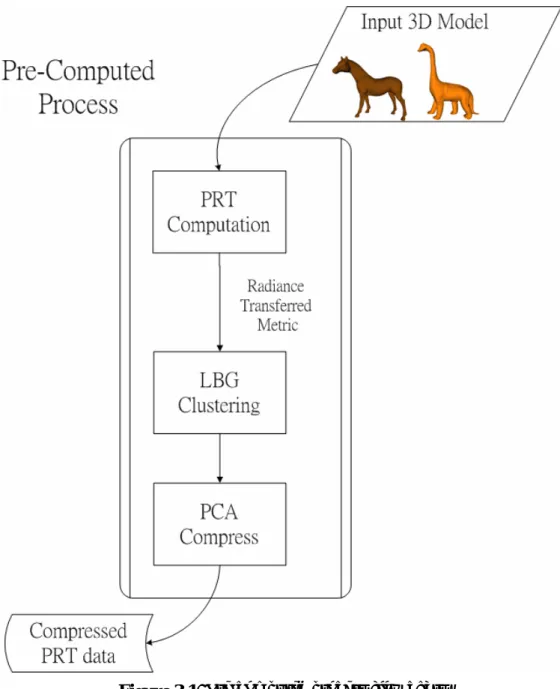
Our system consists of two major processes, one is the pre-computed process and the other is rendering process. The input of pre-computed process is a 3D model. After the pre-computed process, the outputs are the principle component of radiance transfer matrices. The principle component of radiance transfer matrices is also one of the inputs of rendering process. After the rendering process, the lighting transport results of the 3D model are displayed on the screen. In this chapter, we will discuss these two processes individually.

(23)

Figure 3.1: Pre-computed process flow chart

A 3D model is the input of the pre-computed process. The outputs of the PRT computation module are the PRT vector of each vertex. The PRT vector of each vertex is given by projecting the radiance transfer matrix to the SH basis domain. The PRT vectors of all vertices form the inputs of the LBG cluster module. The LBG cluster module classifies the inputs into several clusters. After LBG cluster module,

(24)

output compressed data is saved for rendering process. We will describe the three modules in the following.

3.1.1 PRT computation module

The PRT computation of radiance transfer matrices is proposed by Sloan et al. [22]. They separated the measurement process into two passes: the shadow pass and the light transport pass. The shadow pass measures the direct shadow effect. The light transport pass measures the lighting effects, such as reflections and transmissions.

First, in the shadow pass, we get the visibility map V for each vertex. The _p

visibility map is measured by setting view position at vertex p and render mesh into the cubic map. Next, sample the visibility map in direction sd. sd only needs the

directions around the vertex normal above the hemi-sphere. The shadow transfer matrix is measured by integrating all directions above the hemi-sphere. The equation is shown below Equation 1.

(25)

“j” equals to l’(l’+1)+m’+1. ym(s)

l means that the m-th projected SH coefficient of

order l in direction s. np is the normal of the vertex p.

Before measuring light transport pass, we need to project BRDF to SH basis domain. Westin et al. [25] proposed a Monte Carlo technique to compute the BRDF matrix, B. The z-axis is the vertex normal and the y-axis is the tangent vector of the vertex. Then we project the BRDF matrix to SH basis.

In the visibility map, there are three situations: entirely shadowed, entirely un-shadowed, and partially shadowed. When measuring light transport pass, we only need to measure the directions which are partially shadowed. We update the transfer matrix from 0

ij

p)

(M iteratively, as shown below Equation 2 and 3.

∫

∈ + = S s p m l 1 -b ij p b ij p ) (M ) (1-Vp(s))y (s)IR (s)ds (M (2)

(

)

{

}

∑

= = 2 l" 1 k m" l" kj 1 -b q q p(s) R (B)(M ) y (-s) IR (3) b ij p )

(M is the final radiance transfer matrix of vertex p. “q” is the hitting point of sample ray from vertex p to another triangle in direction s. R_q(B)denotes the rotated

BRDF matrix where the coordinate is aligned the local coordinate of the vertex. If the object does not consider the light transmission effect, we only need to integrate over the hemi-sphere. ”b” is a user defined value which is the maximum number of

(26)

iterations for measuring radiance transfer matrix.

3.1.2 LBG clustering module

The PRT computation module measures the radiance transfer matrix of each vertex and projects to the SH basis. The inputs of the LBG clustering module are the projected coefficients. The projected coefficients of each vertex are called the PRT vector. For all vectors, we cluster the data using the LBG algorithm [13]. The LBG clustering algorithm is also called k-means clustering algorithm [20], where “k” means the data will be clustered into k clusters. The pseudo code of LBG algorithm is shown in Figure 3.2.

Step 0: Initial pass:

For each cluster, randomly give the mean value. Step 1: Cluster pass:

For each vector, find the nearest cluster by calculating distance of mean. Step 2: Update pass:

For each cluster, update the mean by average the vectors which belong to the cluster.

(27)

The total energy of all vertices Ei is defined as following Equation 4. The “i”

means i-th iteration. The distance of mean is the Gaussian distance.

∑

∈ = = vertex all v v 2 v d Ei || Mean -V || d v (4)

The converged ratio is defined in Equation 5. When the ratio is less than a user defined threshold, the LBG clustering algorithm is done. In our system, another converged state is occurred when the total energy function equals to zero. It may occur when all data is the same.

∞ = = 0 1 -i i 1 -i E )/E E -(E R (5)

The traditional LBG algorithm initializes means by randomly sampled values. It may take unnecessary iterations to converge the state. So, in our system, we first scan all vertices to find the hyper-box of all data. The idea of hype-box is similar to the bounding box, where the difference is that the dimension of hyper-box is greater than 3. Then we randomly pick up several points in hyper-box as initial cluster means.

Furthermore, the LBG algorithm may result another problem, called “Null Cluster”, even though the state converged. The “Null Cluster” means that no data belongs to this cluster after clustering algorithm done. It is because that we pick up

(28)

points randomly. To solve this in our system, we will find a cluster, which includes more data than any other clusters, when the null cluster occurred. Then we divide the data into two clusters. The total energy is surely less than the original energy. The “Null Cluster Avoidance” is still applied until there are none “Null Cluster”. After LBG clustering module, the original data are partitioned into several clusters.

3.1.3 PCA compressing module

After LBG clustering module, we apply PCA to each cluster. The PCA compressing module will analyze the data and find the principle components. The number of principle components is given by user. In practice, we often use 8 or 12 principle components for each cluster. After PCA for each cluster, we will get the principle components for a cluster and get the weighting coefficients vector for each vertex in the cluster. In rendering time, we will reconstruct the PRT vectors by weighting coefficients vector and principle components. The equation is shown as following Equation 6.

(29)

number of the principle components the less approximating distortion. The “Mk” is

the mean of the cluster. The “wpj” is the weighting coefficients vector of vertex p. The

“Bj” is the principle components of the cluster. For the vertices in each cluster, “Mk”

and “Bj” is the same. For each vertex, it only need restore “wpj” and which cluster it

belongs to.

After this module, the required storage is decreased. The required storage of the PRT vectors is (NumberOfVertice * VectorSize). After the PCA compressing module, the required storage is ( NumberOfVertice * NumberOfPC + NumberOfCluster * (NumberOfPC +1)* VectorSize ).

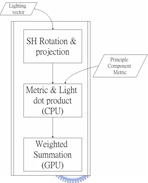
3.2 Rendering process

In this section, we describe the rendering process. The flow chart of rendering process is shown as Figure 3.3.

(30)

Figure 3.3: The rendering process flow chart

There are also three components in this process. The inputs of the process are lighting vector and principle component matrices. The lighting vector is obtain by

(31)

Before calculating the dot product of vectors and lighting vector, we need to rotate the light vector. It is because that the lighting environment is dynamic. The environment can be rotated arbitrarily. Since the light source came from infinite, the movement of environment need not concern. Although we can re-project light source to SH basis again when the lighting environment changed, but it takes expensive computation for rendering. Ivanic et al. [6][7] proposed a method to rotate the SH coefficients in the SH domain. The computation cost is less than re-projecting lighting vector to SH basis. We also apply their method in our system.

After pre-computed process, we get the principle components of clusters and the weighting vectors of all vertices. In the original PRT, we need to calculate the dot product of the PRT vectors and lighting vector to get the lighting effect. After compression, we only need to calculate the dot product of the principle components and the lighting vector, and weighted summation by weighting vector. The equation is shown as follows: Equation 7.

∑

• ⋅ + • ≈ • ⇒ ⋅ + ≈ j j pj k p j j pj k p L B w L M L R B w M R (7)

In our system, we calculate the dot product Mk‧L and Bj‧L in CPU and the

(32)

fragment shader model 3.0 and do per-vertex computation. The principle component metric are placed in the hardware float constant registers. The weighting vector of each vertex is placed as the input of the shader. We use the High Level Shading Language (HLSL) to utilize the shader to compute the weighted summation. The other points on the mesh surface except mesh vertices will shade by hardware interpolation.

(33)

Chapter 4 Triangles Overdraw Reduction

In this chapter, we discuss the triangles overdraw problem and introduce two methods to reduce it. First in Section 4.1, we introduce the triangles overdraw problem. In Section 4.2, we apply the Geometry Coherence to decrease the triangles overdraw. In Section 4.3, we introduce a cluster selection algorithm for super-cluster to reduce triangles overdraw.

4.1 The triangles overdraw problem

The triangles overdraw problem means that triangles are drawn over more than one time when rendering. This problem is occurred as a result of the current graphic hardware restriction. Recalling in Chapter 3, we cluster the PRT vectors into several clusters and place the principle components into the graphic card registers. If the number of clusters is large enough, the registers requirement of all principle components may be larger than the number of graphic hardware registers. Therefore

(34)

the objects are not rendered in one pass. Some triangles could be rendered in the second or third passes. For example, the modern graphic hardware equips with 256 float4 registers (i.e. float4 register equals 4 float registers). If we use order 6 SH basis for glossy objects, 8 principle components per cluster. The PRT vectors are classified into 60 clusters. The requirement of registers is ((6*6)*(8+1)*60)/4, i.e. 4860, float4 registers is larger than 256 float4 registers.

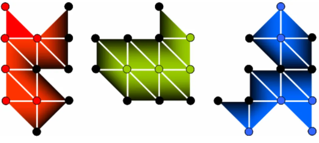
In our system, we will split the mesh into several partitions by distribution of clusters. When rendering, we accumulate all rendering result of partitions to get the final result. For example in Figure 4.1, the mesh is divided into three clusters and represented by three colors, red, blue, and green respectively.

(35)

The mesh will be split into three partitions, as shown in Figure 4.2.

Figure 4.2: Mesh Partitions

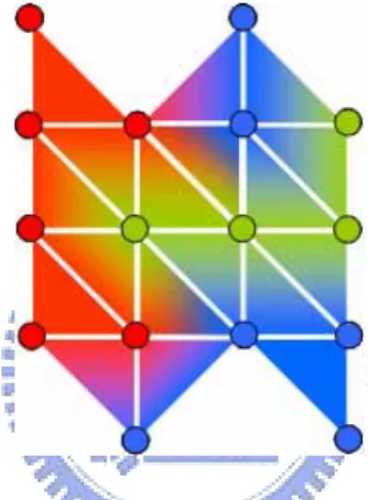
When rendering vertices of triangles in a cluster, there are two situations occurred. One is the vertex belong to current cluster. We will calculate the lighting effect of the vertex. The other is the vertex belong to another cluster. We will set the output lighting effect result to zero (i.e. black color). After all clusters are rendered, all vertices lighting effect are calculated. The triangles overdraw occurs. Figure 4.3 shows all triangles overdraw of the example mesh.

(36)

There are three situations of triangle overdraw. First, the triangle overdraws equals to one, it means that the vertices of triangle belong to the same cluster. Second, the triangle overdraws equal to two, it means that the vertices of the triangle belong to two clusters. The triangle will be drawn in two times. Third, the triangle overdraws equals to three, it means that the vertices of the triangle belong to three clusters, and the triangle will draw in three times. The accumulated result is shown in Figure 4.4.

Figure 4.4: Accumulated mesh result

In our system, we apply alpha blending function in graphic card to accumulate the result of partitions. We measure the “average triangle overdraws” in our system to represent the triangles overdraw instead of total rendering triangles. The average

(37)

In the result, we compare the rendering speed by listing the average triangles overdraw and frames per second (FPS). The average triangles overdraw will affect the rendering speed directly.

4.2 The geometry coherence

In Chapter 3, we cluster the PRT vectors by calculating the Gaussian distances between the PRT vector and mean vectors of clusters. Some vertices may cluster into a clusters but not close in 3D space. It will increase the extra triangle overdraws. The geometry coherence is an idea to reduce the extra triangle overdraws. The main concept of geometry coherence is that” When the vertices are closer, the PRT vectors are similar”. In our system, we add the geometry coherence in the LBG clustering algorithm module. When clustering the PRT vectors, we not only calculate the Gaussian distances of vectors but also calculate the Gaussian distances of positions.

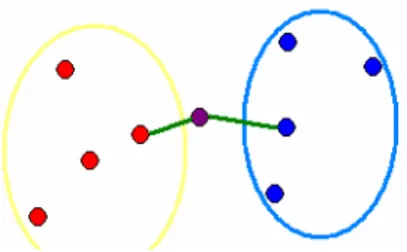
For example in Figure 4.5, the purple point is the data point we want to cluster. The red points are in one cluster and blue points are in another cluster.

(38)

Figure 4.5: The Geometry Coherence example

In our system, we cluster the data by calculating the Gaussian distances of PRT vector plus the Gaussian distances of position vector. The equation is shown as following. j j i ij V -mean GeoCoherence E = v +α⋅ (9)

The “i” means point i-th and the “j” means the j-th cluster. “α” is a user given

value to control the effect of geometry coherence. The “GeoCoherence” is defined as

finding the minimum distance of the data and the points in a cluster. The equation is shown as following. } P -P { min ce GeoCoheren _i _k j cluster k point j v v ∈ ∀ = (10)

(39)

4.3 The clusters selection algorithm

Sloan et al. [21] introduces the idea of super-clusters to reduce the triangles overdraw. But they don’t give a proper method for selecting the clusters for super-clusters. In the following, we discuss a clusters selection algorithm for super-clusters.

In the Section 4.1, we discuss the reason of triangles overdraw. Although we can not place all clusters in one pass, but we can place partial clusters of all in one pass. Recalling the example in Section 4.1, if we want to place all clusters into registers, we need 4860 float4 registers. The registers requirement of one cluster is 81 float4 registers. So we can place 256/81, 3 clusters in one pass rendering. This is the main concept of super-clusters. Our goal is to establish an algorithm to select clusters for a super-cluster. This will reduce the triangle overdraw again.

(40)

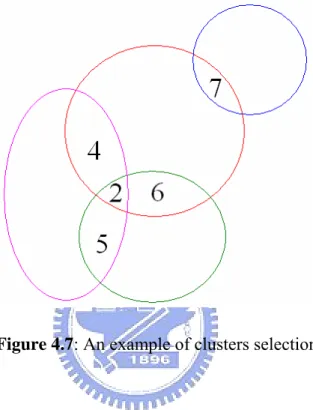
Figure 4.6: The clusters selecting algorithm for super-clusters

In step 3, “merge the cluster” does not mean merge the principle component data of two clusters. It means that we will concern both triangle overdraw reduction effect in the next time selecting another cluster, i.e. Step 2.

For example, in Figure 4.7, every circle represents a cluster. The intersection of two circles means the reduced triangle overdraws when they are selected into the

Step 1: Find the cluster which has the most data and put in cluster C.

Step 2: Find the cluster which can reduce the most triangles overdraws of cluster C.

Step 3: Merge the cluster selected by step 2 into cluster C.

Step 4: If all clusters are selected, then exit.

Else if the registers are full, then go to step 1 and empty the cluster C.

(41)

cluster because the purple cluster will reduce more triangle overdraws. So, the “merge” means merging the triangle overdraw reduction effects when we select another cluster into a super-cluster in the next iteration.

(42)

Chapter 5 Experimental Results

In this chapter, we demonstrate experimental results of our purposed approach. Our system is implemented in C++ language and DirectX 9.0c [16]. It is working on a Pentium IV 3.4GHz CPU and an NVIDIA GeForce 6800GT graphic card.

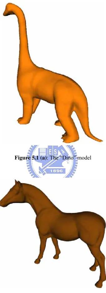
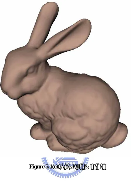
In the testing examples, we compare our results with two previous methods which are the original CPCA method and the CPCA triangle overdraws reduced method. The resolution of image size is 1280 × 948 pixels. All the testing models are shown in the Figure 5.1. Table 5.1 shows the details of these models. The first row refers to the number of vertices of them. The second row refers to the number of

(43)

Figure 5.1 (a): The “Dino” model

(44)

Figure 5.1(c): The “Bunny” model

Dino Horse Bunny

Vertices 23984 19851 34834 Triangles 47904 39698 69451

(45)

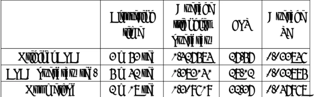
In the following tables, the first column refers to the methods. The second column refers to the clustering time in LBG algorithm module. The third column refers to the average triangles overdraw. The last column refers to the frames per second (FPS). The fifth column refers to the average squared error (SE).

First, the measurement of the “Dino” model is shown as follows. The material is applying Phong BRDF model. Table 5.2 shows the comparison with the other methods where the number of clusters is 64. Figure 5.2 shows the rendering result. Figure 5.2 (a) shows the uncompressed rendered result. Figure 5.2 (b) shows the rendered result of the original CPCA method without applying triangle overdraws reduction. Figure 5.2 (c) shows the result with applying triangle overdraws reduction. Figure 5.2 (d) shows the rendered result which applies our method.

Clustering time Average triangles overdraw FPS Average SE Original CPCA 3 m 53 sec 1.427584 27.57 0.033846 CPCA overdraw red. 5 m 42 sec 1.383141 28.12 0.032895 Our method 2 m 18 sec 1.309619 32.37 0.047968

(46)

(a): uncompressed result (b): original CPCA method

(c): CPCA triangles overdraw red. (d): our method

(47)

Clustering time Average triangles overdraw FPS Average SE Original CPCA 27 m 4 s 1.733425 22.93 0.005371 CPCA overdraw red. 27 m 27 s 1.646063 24.43 0.006344 Our method 7 m 31 s 1.404810 30.52 0.012216

Table 5.3: The “Dino” model, 256 clusters, α=0.05

(a): Uncompressed result (b): Original CPCA method

(c): CPCA triangles overdraw red. (d): Our method

(48)

Similarly the result for 128 and 192 clusters are shown in Tables 5.4 and 5.5 respectively. Clustering time Average triangles overdraw FPS Average SE Original CPCA 12 m 38 s 1.556363 26.58 0.014452 CPCA overdraw red. 12 m 17 s 1.505114 27.15 0.014756 Our method 4 m 10 s 1.359051 31.91 0.027246

Clustering time Average triangles overdraw FPS Average SE Original CPCA 15 m 15 s 1.637316 24.62 0.007938 CPCA overdraw red. 19 m 46 s 1.593019 25.60 0.008764 Our method 4 m 55 s 1.382953 30.89 0.017335

Next example is a “Horse” model. The material is applying the Phong BRDF model. Table 5.6 shows the comparing results, where the number of clusters is 64. Figure 5.4 displays the rendering results.

(49)

Clustering time Average triangles overdraw FPS Average SE Original CPCA 3 m 46 s 1.510882 27.70 0.029795 CPCA overdraw red. 4 m 19 s 1.449997 29.38 0.029944 Our method 5 m 44 s 1.417578 30.51 0.029789 CPCA overdraw red.

+ Our method 4 m 30 s 1.344148 32.11 0.030263

Table 5.6: The “Horse” model, 64 clusters, α=0.05

Figure 5.4: The “Horse” model comparisons, 64 clusters

(50)

Clustering time Average triangles overdraw FPS Average SE Original CPCA 16 m 1.825407 25.18 0.006340 CPCA overdraw red. 16 m 56 s 1.724545 27.70 0.007333 Our method 20 m 17 s 1.632803 30.03 0.006301 CPCA overdraw red.

+ Our method 13 m 40 s 1.574815 32.54 0.007226

(51)

+ Our method 6 m 9 s 1.474205 32.47 0.015547

+ Our method 13 m 54 s 1.511764 31.16 0.010184

Next, we apply the Cook-Torrance BRDF model [2]. Table 5.10 shows the result where the number of clusters is 64. Figure 5.6 shows the rendering results.

+ Our method 3 m 4 s 1.378961 31.59 0.259388

(52)

Next for 256 clusters, the results are shown in Table 5.11 and Figure 5.7.

Clustering time

Average

triangles FPS Average SE

(53)

For 128 and 192 clusters, Tables 5.12 and 5.13 show the results.

+ Our method 9 m 22 s 1.457983 31.62 0.136876

(54)

+ Our method 12 m 4 s 1.560885 30.24 0.092139

Finally, we use the “Bunny” model for testing. We apply the Cook-Torrance BRDF model. Table 5.14 shows the results for 256 clusters. Figure 5.8 shows the rendering results. Clustering time Average triangles overdraw FPS Average SE Original CPCA 26 m 49 s 1.529308 23.05 0.054466 CPCA overdraw red. 31 m 26 s 1.467294 24.45 0.058319 Our method 38 m 13 s 1.413759 25.89 0.054501 CPCA overdraw red.

+ Our method 34 m 47 s 1.378627 26.77 0.055894

(55)

Figure 5.8: The “Bunny” model comparisons, 256 clusters

Tables 5.15, 5.16, and 5.17 show the results of 64 clusters, 128 clusters, and 196 clusters. Clustering time Average triangles overdraw FPS Average SE Original CPCA 5 m 40 s 1.305410 25.86 0.221043 CPCA overdraw red. 7 m 18 s 1.275172 26.67 0.224016 Our method 10 m 6 s 1.239781 27.72 0.221096 CPCA overdraw red.

(56)

+ Our method 17 m 17 s 1.285856 28.16 0.113184

Table 5.16: The “Bunny” model, 128 clusters, α=0.05

+ Our method 22 m 35 s 1.337691 27.83 0.077189

Table 5.17: The “Bunny” model, 192 clusters, α=0.05

Next, we change the lighting condition to the environment lighting. We show the rendering results in the following figures.

(57)

Figure 5.9: The “Horse” model with environment lighting

(58)

Chapter 6 Conclusions and Future Works

In this thesis, we propose two methods to reduce the triangles overdraw. One considers Geometry Coherence and the other uses the clusters selection algorithm.

Geometry Coherence may reduce the triangle overdraws, but increase the average square errors. Although the average square errors increase, the rendered images do not differ very much perceptually.

The clusters selection algorithm may also reduce the triangle overdraws. The number of clusters for a super-cluster will affect the number of reduced triangle overdraws. When the number of clusters for a super-cluster is smaller, the number of reduced triangle overdraws is smaller. Oppositely, when the number of clusters for a super-cluster is larger, the number of reduced triangle overdraws is larger.

(59)

Our proposed approaches increase the real-time performance of global illumination. Our approaches can be applied to 3D games or virtual reality applications.

However, there are still some issues left for future research.

(1) There could be other coherences may enhance the performance further.

(2) The Geometry Coherence may increase the average squared error. We may try another approach to control the average squared error.

(3) The LBG algorithm is a simple clustering method. We may try to find another clustering algorithm to decrease the clustering time.

(60)

References

[1] CHEN, W.-C., BOUGUET, Y.-V., CHU, M. H., AND GRZESZCZUK, R. 2002. Light Field Mapping: Efficient Representation and Hardware Rendering of Surface Light Fields. ACM Transactions on Graphics, 21(3), 447-456.

[2] COOK, R. AND TORRANCE, K. 1982. A Reflectance Model for Computer Graphics. ACM Transactions on Graphics, 1(1), 7–24.

[3] DANA, K, VAN GINNEKEN, B, NAYAR, S, AND KOENDERINK, J. 1999. Reflectance and Texture of Real World Surfaces. ACM Transactions on Graphics, 18(1), 1-34.

[4] GORAL, C. M., TORRANCE, K. E., GREENBERG, D. P., AND BATTAILE, B. 1984. Modeling the Interaction of Light between Diffuse Surfaces. Proceedings of SIGGRAPH ‘84, 213-222.

[5] GORTLER, S. J., GRZESZCZUK, R., SZELISKI, R., AND COHEN, M. F. 1996. The Lumigraph. Proceedings of SIGGRAPH ‘96, 43-54.

[6] IVANIC, J. AND RUEDENBERG, K. 1996. Rotation Matrices for Real Spherical Harmonics, Direct Determination by Recursion. Journal of Physical Chemistry A, 100(15), 6342-6347.

[7] IVANIC, J. AND RUEDENBERG, K. 1998. Additions and Corrections: Rotation Matrices for Real Spherical Harmonics. Journal of Physical Chemistry A, 102(45), 9099-9100.

(61)

[11] LEHTINEN, J. AND KAUTZ, J. 2003. Matrix Radiance Transfer. Proceedings of the ACM Symposium on Interactive 3D Graphics 2003, 59-64.

[12] LEVOY, M. AND HANRAHAN, P. 1996. Light Field Rendering. Proceedings of SIGGRAPH ‘96, 31-41

[13] LINDE, Y., BUZO, A., AND GRAY, R. 1980. An Algorithm for Vector Quantizer Design, IEEE Transactions on Communication, 28(1), 84-95.

[14] LIU, X., SLOAN, P.-K., SHUM, H.-Y., AND SNYDER, J. 2004. All-Frequency Precomputed Radiance Transfer for Glossy Objects. Proceedings of the Eurographics Symposium on Rendering 2004, 337-344.

[15] MATUSIK, W., PFISTER, H., NGAN, A., BEARDSLEY, P., ZIEGLER, R., AND MCMILLAN L. 2002. Image-Based 3D Photography using Opacity Hulls. ACM Transactions on Graphics, 21(3), 427- 437.

[16] MICROSOFT. 2005. DirectX 9.0c SDK (April 2005).

http://www.microsoft.com/DirectX.

[17] MILLER, G., RUBIN, S., AND PONCELEN, D. 1998. Lazy Decompression of Surface Light Fields for Pre-computed Global Illumination. Proceedings of the Eurographics Workshop on Rendering ‘98, 281- 292.

[18] NG, R., RAMAMOORTHI, R., AND HANRAHAN, P. 2003. All-Frequency Shadows Using Non-Linear Wavelet Lighting Approximation. ACM Transactions on Graphics, 22(3), 376-381.

[19] NG, R., RAMAMOORTHI, R., AND HANRAHAN, P. 2004. Triple Product Wavelet Integrals for All-Frequency Relighting. ACM Transactions on Graphics, 23(3), 477–487

[20] SELIM, S. Z. AND ISMAIL, M. A. 1984. K- Means-Type Algorithms: A Generalized Convergence Theorem and Characterization of Local Optimality. IEEE Transactions on Pattern Analysis and Machine Intelligence, 6(1), 81-87.

(62)

[21] SLOAN, P., HALL, J., HART, J., AND SNYDER, J. 2003. Clustered Principal Components for Pre- computed Radiance Transfer. ACM Transactions on Graphics, 22(3), 382-391.

[22] SLOAN, P., KAUTZ, J., AND SNYDER, J. 2002. Precomputed Radiance Transfer for Real-Time Rendering in Dynamic, Low-Frequency Lighting Environments. ACM Transactions on Graphics, 21(3), 527-536.

[23] SLOAN, P., LIU, X., SHUM, H., AND SNYDER, J. 2003. Bi-Scale Radiance Transfer. ACM Transactions on Graphics, 22(3), 370-375.

[24] VASILESCU, M. A. O. AND TERZOPOULOS, D. 2004. TensorTextures: Multilinear Image-Based Rendering. ACM Transactions on Graphics, 23(3), 336-342.

[25] WESTIN, S., ARVO, J., AND TORRANCE, K. 1992. Predicting Reflectance Functions from Complex Surfaces. Proceedings of SIGGRAPH ‘92, 255-264. [26] WHITTED, T. 1980. An Improved Illumination Model for Shaded Display.

Communications of the ACM, 23(6), 343–349.

[27] WOOD, D., AZUMA, D., ALDINGER, K., CURLESS, B., DUCHAMP, T., SALESIN, D., AND STUETZLE, W. 2000. Surface Light Fields for 3D Photography. Proceedings of SIGGRAPH 2000, 287- 296.

一個事先計算輻射傳輸為基礎的即時全域照度演算法

國

立

交

通

大

學

資訊科學系

碩

士

論

文

一個事先計算輻射傳輸為基礎的

即時全域照度演算法

A Real-Time Global Illumination Algorithm based on

Pre-Computed Radiance Transfer

研 究 生：陳志豪

一 個 事 先 計 算 輻 射 傳 輸 為 基 礎 的 即 時 全 域 照 度 演 算 法

A Real-Time Global Illumination Algorithm based on

Pre-Computed Radiance Transfer

研 究 生：陳志豪 Student：Chin-Hao Chen

指導教授：施仁忠 Advisor：Zen-Chung Shih

國 立 交 通 大 學

資 訊 科 學 系

碩 士 論 文

一個事先計算輻射傳輸為基礎的即時全域照度演算法

研究生: 陳志豪

指導教授: 施仁忠 教授

國立交通大學資訊科學系

摘 要

A real-time global illumination algorithm based on

pre-computed radiance transfer

Student:

Chin-Hao Chen

Advisor: Dr. Zen-Chung Shih

Department of Computer and Information Science

National Chiao-Tung University

ABSTRACT

Acknowledgements

Contents

List of Tables

List of Figures

Chapter 1

Introduction

1.1

Motivation

1.2

Overviews

1.3

Thesis Organization

Chapter 2

Related Works

2.1

Illumination methods

2.2

Survey of PRT Extensions

2.3

PRT approximation methods

2.4

PRT compress method

Chapter 3

System overview

3.1.1

PRT computation module

∫

(

)

{

}

∑

3.1.2 LBG clustering module

∑

3.1.3

PCA compressing module

3.2 Rendering process

∑

∑

Chapter 4

Triangles Overdraw Reduction

4.1

研究生：陳志豪

一個事先計算輻射傳輸為基礎的即時全域照度演算法

研究生：陳志豪 Student：Chin-Hao Chen

國立交通大學

資訊科學系

碩士論文

指導教授: 施仁忠教授

摘要