國 立 交 通 大 學
電 機 與 控 制 工 程 學 系
碩 士 論 文
三層類神經網路的改良式動態最佳學習
Revised Dynamic Optimal Training of Three-Layer
Neural Network
研究生:林書帆
指導教授:王啟旭 教授
三層類神經網路的改良式動態最佳學習
Revised Dynamic Optimal Training of Three-Layer Neural
Network
研究生: 林書帆 Student: Shu-Fan Lin 指導教授:王啟旭 教授 Advisor: Chi-Hsu Wang
國 立 交 通 大 學 電機與控制工程學系
碩士論文
A Thesis
Submitted to Department of Electrical and Control Engineering College of Electrical Engineering and Computer Science
National Chiao Tung University in Partial Fulfillment of the Requirements
for the Degree of Master in
Electrical and Control Engineering October 2006
Hsinchu, Taiwan, Republic of China
三層類神經網路的改良式動態最佳學習
研究生:林書帆 指導教授:王啟旭 教授
國立交通大學電機與控制工程研究所
摘要
本篇論文是針對三層類神經網路提出一個改良式動態最佳訓練法則,其中類神經 網路的隱藏層經過一個 S 型激發函數,輸出層經過一個線性的激發函數。這種三 層的網路可以被運用於處理分類的問題,像是蝴蝶花的品種分類。我們將對這種 三層神經網路的動態最佳訓練方法提出一個完整的証明,用來說明這種動態最佳 訓練方法保證神經網路能在最短的迭代次數下達到收斂的輸出結果。這種改良式 動態最佳訓練方法,是在每一次的迭代過程中不斷的尋找,來取得下一次迭代過 程所需要的最佳學習速率以及穩定學習速率的上限值,以保證最佳的收斂的訓練 結果。經由調整初始加權值矩陣,改變激發函數,改良式動態最佳學習法則比原 先的動態最佳學習法則更加省時以及更加穩定。我們可以由 XOR 和蝴蝶花的測試 例子得到良好的結論。Revised Dynamic Optimal Training of Three-Layer Neural
Network
Student: Shu-Fan Lin Advisor: Chi-Hsu Wang
Department of Electrical and Control Engineering National Chiao Tung University
ABSTRACT
This thesis proposes a revised dynamic optimal training algorithm for a three layer neural network with sigmoid activation function in the hidden layer and linear activation function in the output layer. This three layer neural network can be used for classification problems, such as the classification of Iris data. Rigorous proof has been presented for the revised dynamical optimal training process for this three layer neural network, which guarantees the convergence of the training in a minimum number of epochs. This revised dynamic optimal training finds optimal learning rate with its upper-bound for next iteration to guarantee optimal convergence of training result. With modification of initial weighting factors and activation functions, revised dynamic optimal training algorithm is more stable and faster than dynamic optimal training algorithm. Excellent improvements of computing time and robustness have been obtained for XOR and Iris data set.
ACKNOWLEDGEMENT
I feel external gratitude to my advisor, Chi-Hsu Wang for teaching me many things. He taught me how to do the research and write a thesis. And the most important is that he taught me how to get along with people. And I am grateful to everyone in ECL. I am very happy to get along with you. Finally, I appreciate my parent’s support and concern; therefore I can finish my master degree smoothly.
TABLE OF CONTENTS
摘要...i
ABSTRACT...ii
ACKNOWLEDGEMENT ... iii
TABLE OF CONTENTS ...iv
LIST OF TABLES ...v
LIST OF FIGURES ...vi
CHAPTER 1 Introduction...1
CHAPTER 2 Neural Network and Back-Propagation Algorithm ...4
2.1 Models of A Neuron...4
2.2 Single Layer Perceptron...8
2.3 Multi-layer Feed-forward Perceptron ...10
2.4 The Back-Propagation Algorithm (BPA) ...12
2.5 Dynamic optimal training algorithm of a Three-layer Neural Network ....18
2.5.1 The Architecture of A Three-Layer Network...19
2.5.2 Updating Process of a Three Layer Neural Network...20
2.5.3 Dynamical Optimal Training via Lyapunov’s Method ...21
CHAPTER 3 ...24
Dynamic Optimal Training Algorithm of A Three-Layer Neural Network with Better Performance ...24
3.1 Problems in the Training of Three Layer Neural Network ...25
3.2 Simplification of activation function ...27
3.3 Selection of Initial Weighting Factors ...28
3.4 Determine the upper-bound of learning rate in each iteration ...34
3.5 Conclusion ...42
CHAPTER 4 Experimental Results ...45
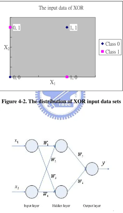
4.1 Example 1: The XOR problem ...45
4.1.1 System modeling and Problem definition...45
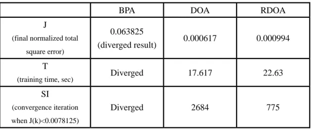
4.1.2 Experimental result analysis ...47
4.2 Example 2: Classification of Iris Data Set...56
4.2.1 System modeling and Problem definition...56
4.2.2 Experimental result analysis ...59
CHAPTER 5 Conclusions...72
REFERENCES ...73
APPENDIX A...77
LIST OF TABLES
TABLE 3-1 OUTPUT OF SIGMOID FUNCTION IN HIDDEN LAYER ...34
TABLE 4-1 TRAINING RESULTS OF XOR PROBLEMS WITH BPA, DOA, RDOA ...47
TABLE 4-2 DETAILED TRAINING RESULTS OF XOR PROBLEMS WITH BPA ...52
TABLE 4-3 DETAILED TRAINING RESULTS OF XOR PROBLEMS WITH DOA ...53
TABLE 4-4 DETAILED TRAINING RESULTS OF XOR PROBLEMS WITH RDOA ...54
TABLE 4-5 THE TRAINING RESULT FOR XOR USING RDOA ...55
TABLE 4-6 THE TRAINING RESULT FOR XOR USING DOA ...55
TABLE 4-7 TRAINING RESULTS OF IRIS WITH BPA, DOA, RDOA...60
TABLE 4-8 DETAILED TRAINING RESULTS OF IRIS WITH BAP ...64
TABLE 4-9 DETAILED TRAINING RESULTS OF IRIS WITH DOA...65
TABLE 4-10 DETAILED TRAINING RESULTS OF IRIS WITH RDOA...66
TABLE 4-11 ACTUAL AND DESIRED OUTPUTS AFTER 10000 TRAINING ITERATIONS ...67
LIST OF FIGURES
FIGURE 2-1 MODEL OF A NEURON ...4
FIGURE 2-2 ANOTHER MODEL OF A NEURON ...6
FIGURE 2-3 (A) THRESHOLD FUNCTION (B) PIECEWISE-LINEAR FUNCTION (C) SIGMOID FUNCTION FOR VARYING SLOPE PARAMETER A...8
FIGURE 2-4 SINGLE LAYER PERCEPTRON...9
FIGURE 2-5 A THREE LAYER FEED-FORWARD NETWORK ... 11
FIGURE 2-6 THE SIGNAL-FLOW GRAPH OF MULTI-LAYER PERCEPTRON ...14
FIGURE 2-7 THREE-LAYER NEURAL NETWORK...19
FIGURE 3-1 THE SIGMOID FUNCTION...25
FIGURE 3-2 NEURAL NETWORK FOR EXAMPLE 3-1...33
FIGURE 3-3 REVISED THREE LAYER NEURAL NETWORK ...34
FIGURE 3-4 NEURAL NETWORK FOR EXAMPLE 3-2...42
FIGURE 4-1 THE TRUTH TABLE OF XOR FUNCTION: Y = A ♁ B...45
FIGURE 4-2 THE DISTRIBUTION OF XOR INPUT DATA SETS ...46
FIGURE 4-3 THE NEURAL NETWORK FOR SOLVING XOR...46
FIGURE 4-4 NORMALIZED SQUARE ERROR J OF THE BPA WITH FIXED RATE = 0.9 ...49
FIGURE 4-5 THE BEST NORMALIZED SQUARE ERROR J OF THE DOA IN 20 TRIALS...50
FIGURE 4-6 THE BEST NORMALIZED SQUARE ERROR J OF THE RDOA IN 20 TRIALS ...50
FIGURE 4-7-1 TRAINING ERROR OF RDOA, DOA, AND BPA FOR XOR ...51
FIGURE 4-7-2 THE CLOSE LOOK OF TRAINING ERROR FOR XOR ...51
FIGURE 4-8-1 THE TOTAL IRIS DATA SET (SEPAL) ...57
FIGURE 4-8-2 THE TOTAL IRIS DATA SET (PETAL)...57
FIGURE 4-9-1 THE TRAINING SET OF IRIS DATA (SEPAL) ...58
FIGURE 4-9-2 THE TRAINING SET OF IRIS DATA (PETAL) ...58
FIGURE 4-10 THE NEURAL NETWORK FOR SOLVING IRIS PROBLEM...59
FIGURE 4-11 NORMALIZED SQUARE ERROR J OF THE BPA WITH FIXED RATE = 0.1 ...61
FIGURE 4-12 THE NORMALIZED SQUARE ERROR J OF THE DOA ...62
FIGURE 4-13 THE NORMALIZED SQUARE ERROR J OF THE RDOA...62
FIGURE 4-14-1 TRAINING ERROR OF RDOA, DOA, AND BPA FOR IRIS ...63
CHAPTER 1
Introduction
Artificial neural network (ANN) is the science of investigating and analyzing the
algorithms of the human brain, and using similar algorithm to build up a powerful computational system to do the tasks like pattern recognition [1], [2], identification [3], [4] and control of dynamical systems [5], [6], system modeling [7], [8] and nonlinear prediction of time series [9]. The first model of artificial neural network was proposed for simulating human brain by F. Rosenblatt in 1958, 1962 [10], [11]. So the most attractive character of artificial neural network is that it can be taught to achieve the complex tasks we had experienced before by using some learning algorithms and training examples. Among most popular training algorithms of artificial neural network, Error Back-Propagation Algorithm [12], [13] is widely used for classification problems. The well-known error back-propagation algorithm or simply the back-propagation algorithm (BPA), for training multi-layer perceptrons was proposed by Rumelhart et al. in 1986 [14]. Although the popular back-propagation algorithm is easier to understand and to implement for most applications, it has the problems of converging to local minimum and a slow convergence rate. It is well known that performance of BPA is significantly affected by several parameters, i.e., learning rate, initial weighting factors and activation functions. In this thesis, the effect of each adjustable parameter will be analyzed, in order to find a new training algorithm with better performance compared with BPA.
There are many research works on the learning of multilayer NN with saturated nonlinear activation functions, e.g., sigmoid function. Some researches work on the
authors in [16] state that if activation functions of each layer of multilayer NN are all sigmoid, the back-propagated error signal may be seriously discounted by the saturation region of sigmoid function. Hence, convergence rate of learning will slow down. Although, multilayer linear neural network does not have the problem of saturation, its learning capability is not as good as multilayer sigmoid neural network. To retain the advantages of both kinds of activation function, and to easy the bad effect of they, the architecture with combination of linear and nonlinear activation functions will be proposed in this investigation. We will also propose an adequate analysis and excellent experimental results to support that the learning of NN will have better performance with an unlimited linear activation in output layer and a sigmoid function in hidden layer.
It is well known that initial weighting factors have a significant impact on the performance of multilayer NN. In almost all applications of back-propagation, the initial weighting factors are selected randomly from a problem-dependent range. In the investigation of Hosein et al. in 1989 [17], high initial weighting factors can accelerate convergence rate of learning, but may suffer the problem of local minimum. Low initial weighting factors can be used over a wide range of applications for reliable learning, but convergence rate may slow down. In this thesis, we will propose a clear and definite way to find proper initial weighting factors which can reduce the probability of falling into local minimum on the error surface during the back propagation process.
Learning rate is always the most important adjustable parameter in BPA and other algorithms which are generalized from BPA. Learning rate controls the convergence of the algorithm to an optimal local solution, and it also dominates the convergence rate. Hence, the choice of learning rate is a critical decision for convergence of BPA.
For smaller learning rate, we may have a convergent result. But the speed of the output convergence is very slow and need more number of epochs to train the network. For larger learning rate, the speed of training can be accelerated, but it will cause the training result to fluctuate and even leads to divergent result. However, Rumelhart et
al. did not show how to get a good value for the learning rate in [14]. Since, several
researches have used empirical rule, heuristic methods, and adaptive algorithm to set a good value for leaning rate. The dynamical optimal learning rate was proposed in [18] for a simple two layer neural network (without hidden layers) without any activation functions in the output layer. To break the limited learning capability for the two-layer NN, authors in [19] presented the dynamical optimal learning rate for the three-layer NN with sigmoid activation functions in the hidden and output layers. The basic theme in [18] and [19] is to find a stable and optimal learning for the next iteration in BPA. Cerqueira et al. [20] developed a local convergence analysis made through Lyapunov’s second method for the BPA and supplied an upper bound for the learning rate. Cerqueira et al. also present an adaptive algorithm with upper bound of learning rate in [21]. In this thesis we combine the basic theme in [18] and [19] with upper bound of learning rate presented in [20] and [21] to present a revised dynamic optimal learning rate with dynamic upper bound in this thesis.
The goal of this thesis is to propose a revised dynamic optimal training algorithm based on modifications made for three key parameters, i.e., learning rate, initial weighting factor and activation function. Rigorous proof will be proposed and the popular XOR [22] and Iris data [23], [24] classification benchmarks will be fully illustrated. Excellent results have been obtained by comparing our optimal training results with previous results using fixed small learning rates.
CHAPTER 2
Neural Network and Back-Propagation Algorithm
In this chapter, the multi-layer feed-forward perceptron (MLP) structure of artificial neural networks (ANN) and the training algorithm will be introduced. First the model of a neuron will be introduced. Then, the single layer perceptron will be explained and it will lead to the multi-layer perceptrons in later sections. The back-propagation algorithm for multi-layer feed forward perceptrons will be explained in Section 2.4. Finally, the dynamic optimal training algorithm will be introduced in Section 2.5.
2.1 Models of A Neuron
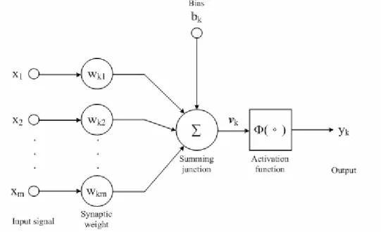
A neuron is an information-processing unit that is fundamental to the operation of a neural network. It is the basic unit in a neural network. It forms the basis for designing artificial neural network. The block diagram of the model of a neuron is shown in Figure 2-1. The neural model can be divided into three basic elements.
1. A set of synaptic links, each of which is characterized by a weight factor. Symbol xj denotes the input signal at the input of synapse j. The input signal xj connected to neuron k is multiplied by the synaptic weight wkj. Symbol wkj denotes the weight factor from jth neuron to kth neuron.
2. An adder for summing the input signals which are weighted by the respective synapses of the neuron. These operations constitute a linear combiner.
3. An activation function for limiting the amplitude of the output of a neuron. The activation function squashes or limits the amplitude range of the output signal to some finite value. It can also set a saturation region for the output signal.
The neuron model of Figure 2-1 also includes an externally applied bias, denoted by bk. The bias bk has the effect of increasing or decreasing the net input of the activation function, depending on whether it is positive or negative, respectively. In mathematical terms, we can describe the model of a neuron k by using the following pair of equations:
1 m k k j j j
v
w x
==
∑
(2.1) and(
)
k k k y =φ
v +b (2.2)where x1, x2, …., xm are the input signals; wk1, wk2, …., wkm are the synaptic weights of neuron k; Vk is the linear combiner output; bk is the bias;φ
( )
is the activation function; and yk is the output signal of the neuron. The bias bk is an external parameter of artificial neuron k. It can be expressed in another form. In Figure 2-1, we add a new synapse, it input is x0 = 1 and its weight is wk0 = bk. We may therefore redefine a newFigure 2-2. Another Model of A Neuron
Activation function φ
( )
defines the output of a neuron k in terms of the induced local field Vk . There are three basic types of activation functions.1. Threshold Function. (Figure 2-3(a))
1 0 ( ) 0 0 if v v if v φ = ⎨⎧ ≥ < ⎩ (2.3)
In this type, the output of a neuron has the value 1 if the induced local field of the neuron is nonnegative and 0 otherwise. The output of neuron k applies into such a threshold function can be expressed as
1 0 0 0 k k k if v y if v ≥ ⎧ = ⎨ < ⎩ (2.4)
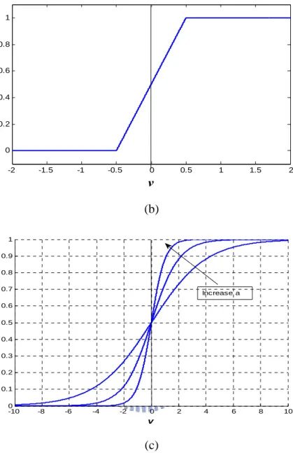
2. Piecewise-Linear Function. (Figure 2-3(b))
1 1 2 1 1 ( ) 0.5 2 2 1 0 2 v v v v v φ ⎧ ≥ + ⎪ ⎪ =⎨ + + > > − ⎪ ≤ − ⎪⎩ (2.5)
This form of an activation function can be viewed as an approximation to a nonlinear amplifier. A linear function can be viewed as the special form of
piecewise-linear function when piecewise-linear function maintains in the linear region of operation without running into saturation.
1. Sigmoid Function. (Figure 2-3(c))
Sigmoid function is the most common form of activation function used in construction of artificial neural network. The graph of sigmoid function is s-shaped. It is defined as a strictly increasing function and it exhibits a graceful balance between linear and nonlinear behavior. A common form of sigmoid function is the
logistics function [25] which is defined by
1 ( ) 1 exp( ) v av φ = + − (2.6)
where a is the slope parameter of the sigmoid function. By varying the slope parameter a, we have different types of sigmoid function. It is noted that the slope at original point equals a/4. A sigmoid function gives a continuous range of values from 0 to 1. Sigmoid function is differentiable over the all range of values, whereas threshold function and piecewise-linear function are not. It is an important fact of neural network theory discussed in the later chapter.
-2 -1.5 -1 -0.5 0 0.5 1 1.5 2 0 0.2 0.4 0.6 0.8 1 v (a)
-2 -1.5 -1 -0.5 0 0.5 1 1.5 2 0 0.2 0.4 0.6 0.8 1 v (b) -10 -8 -6 -4 -2 0 2 4 6 8 10 0 0.1 0.2 0.3 0.4 0.5 0.6 0.7 0.8 0.9 1 v Increase a (c)
Figure 2-3. (a) Threshold function (b) Piecewise-linear function (c) Sigmoid function for varying slope parameter a
2.2 Single Layer Perceptron
The first model of the feed-forward network, perceptron, was proposed by F. Rosenblatt in 1958 [10]. He hoped to find a suitable model to simulate the animal’s brain and the visual system so that he proposed the “perceptron” model, which is a supervised
learning model. The supervised learning is also referred to as the learning with a teacher,
perceptron can be trained by the given input-output data. The perceptron is the simplest form of a neural network used for classification of patterns which are said to be linear
separable. Basically, the structure of the perceptron consists of a neuron with adjustable
synaptic weights, bias, and desired output. The structure of the perceptron is depicted in Figure 2-4. The limiter is using a threshold function; its graph is shown in Figure 2-3(a).
Figure 2-4. Single layer perceptron
In Figure 2-4, the input data set of the perceptron is denoted by {x1, x2,…, xm} and the corresponding synaptic weights of the perceptron are denoted by {w1, w2,…, wm}. The external bias is denoted by b. The first part of the percpetron computes the linear combination of the products of input data and synaptic weight with an externally applied bias. So the result of the first part of the perceptron, v, can be expressed as
1 m i i i v b w x = = +
∑
(2.7) Then in the second part, the resulted sum v is applied to a hard limiter. Therefore, the output of the perceptron equals +1 or 0. The output of perceptron equals to +1 if the resulted sum v is positive or zero; and the output of perceptron equals to 0 if v is negative. This can be simply expressed by (2.8).m i=1 m i=1 1 if + 0 0 if + 0 i i i i b x w y b x w ⎧+ ≥ ⎪⎪ = ⎨ ⎪ < ⎪⎩
∑
∑
, , (2.8) The goal of the perceptron is to classify the input data represents by the set {x1, x2,…, xm}into one of two classes, C1 and C2. If the output of the perceptron equals to +1, the input
data represented by the set {x1, x2,…, xm}will be assigned to class C1. Otherwise, the
input data will be assigned to class C2. The single layer perceptron with only a single
neuron is limited to performing pattern classification with only two classes. By expending the output layer of the perceptron to include more than one neuron, we can perform classification with more than two classes. However, these classes must be linearly separable for the perceptron to work properly. If we need to deal with classes which are not linearly separable, we need multi-layer feed-forward perceptron to handle such classes.
2.3 Multi-layer Feed-forward Perceptron
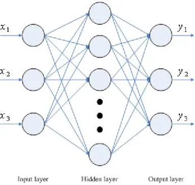
In this section we will introduce the multi-layer feed-forward network, an important class of neural network. The difference between single layer perceptron and multi-layer feed-forward perceptron is the “hidden layer”. The multi-layer network consists of a set of input nodes (input layer), one or more hidden layers, and a set of output nodes that constitute the output layer. The input signals will propagate through the network in the forward direction. A multi-layer feed-forward fully-connected network is shown in Figure 2-5 with only one hidden layer.
Figure 2-5. A three layer feed-forward network
A multi-layer perceptron has three major characteristics:
1. The model of each neuron in the network includes a nonlinear activation function. Note that the activation function used in the multilayer perceptron is smooth, means the activation function is differentiable everywhere. It is different from the threshold function (Figure 2-3(a)) used in the model of single-layer perceptron. A commonly used form of nonlinear activation function is a sigmoid function.
1 1 exp( ) y ax = + −
where x is the induced local field, the weighted sum of all synaptic inputs plus the bias. y is the output of the neuron. And a is the slope parameter of the sigmoid function. Usually, we set the value of a to be 1.
2. The neural network contains one or more layers of hidden neurons between input layer and output layer. The hidden neurons enable the multi-layer networks to deal with more complex problems which can not be solved by single layer perceptron. The number of hidden layers for different problems is also an open question. From
previous researches, one hidden layer is enough to handle many problems properly. Two or more hidden layers can do more complex tasks, but take a huge computation time.
3. The network exhibits a high degree of connectivity. Any change in the connectivity of the network requires a change in the population of synaptic weights. This character makes network more like the human brain.
2.4 The Back-Propagation Algorithm (BPA)
The most serious problem of the single-layer perceptron is that we don’t have any proper learning algorithm to adjust the synaptic weights of the perceptron. But the multi-layer feed-forward perceptron doesn’t have this problem. The synaptic weights of the multi-layer perceptrons can be trained by using the highly popular algorithm known as the error back-propagation algorithm (EBP algorithm) [14]. We can view the error back-propagation algorithm as the general form of the least-mean square algorithm (LMS) [26]. The error back-propagation algorithm (or the back-propagation algorithm) consists of two parts, one is the forward pass and the other is the backward pass. In the forward pass, the effect of the input data propagates through the network layer by layer. During this process, the synaptic weights of the networks are all fixed. On the other hand, the synaptic weights of the multi-layer perceptron are all adjusted in accordance with the error-correction rule during the backward pass. Before using error-correction rule, we have to define the error signal of the learning process. Because the goal of the learning algorithm is to find one set of weights which makes the actual outputs of the network equal to the desired outputs, so we can define the error signal as the difference between the actual output and the desired output. Specifically, the desired response is subtracted from the actual response of the network to produce the error signal. In the backward pass, the error signal propagates backward through the network from output
layer. During the backward pass, the synaptic weights of the multi-layer perceptron are adjusted to make the actual outputs of the network move closer to the desired outputs. This is why we call this algorithm as “error back-propagation algorithm”.
Back-propagation algorithm:
First, we define the error signal at the output of the neuron j at iteration t
( )
( )
( )
j j j
e t = y t −d t (2.9)
where dj is the desired output of output node j and yj is the actual output of output node j. We define the square error of output node j.
( )
2 1 = 2 j e tj ζ (2.10)By the same way, we can define the total square error J of the network as: 2 1 2 j j j j J =
∑
ζ =∑
e (2.11)The goal of the back-propagation algorithm is to find one set of weights so that the actual outputs can be as close as possible to the desired outputs. In other words, the purpose of the back-propagation algorithm is to reduce the total square error J, as described in (2.11). In the method of steepest descent, the successive adjustments applied to the weight matrix W are in the direction opposite to the gradient matrix∂ ∂J/ W . The adjustment of weight matrix W can be expressed as:
(t 1) ( )t ( )t ( )t t J W W W W W η + ∂ = − ∆ = − ∂
( )
t J W t W η ∂ ∆ = − ∂ (2.12)where η is the learning rate parameter of the back-propagation algorithm. It decides the step-size of correction of the method of steepest descent. Note that the learning rate is a positive constant. Fig. 2-6 shows the signal-flow graph of multi-layer perceptron with
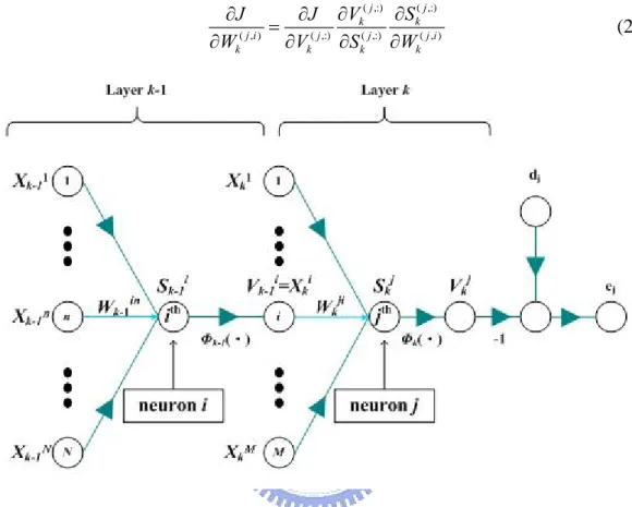
in each layer are assumed to be the same sigmoid function in Fig. 2-6. By using the chain rule, the element of matrix∂ ∂J W, i.e., ∂ ∂J Wk( , )j i , can be represented as:
( ,:) ( ,:) ( , ) ( ,:) ( ,:) ( , ) j j k k j i j j j i k k k k V S J J W V S W ∂ ∂ ∂ ∂ = ∂ ∂ ∂ ∂ (2.13)
Figure 2-6 The signal-flow graph of multi-layer perceptron
where Wk( , )j i is the weight value between the ith neuron in the (k-1)th layer and jth neuron in the kth layer, as shown in Figure 2-6. ϕk
( )
denotes the activation function used in the kth layer. Vk( ,:)j denotes the activation function output of jth neuron in the kth layer. If kth layer is output layer, Vk( ,:)j is equal to yj. Sk( ,:)j denotes the linearcombination output of jth neuron in the kth layer. It can be shown as:
(
)
( ,:)j ( , )j i ( ,:)i
k k k
i
where Xki is the input of neuron in the kth layer. The superscript i means this input comes
from ith neuron in the (k-1)th layer. Note that Xki is also the activation function output of ith
neuron in the (k-1)th layer. So it has another form as: ( ,:) ( ,:)
1
i i
k k
X =V− (2.15)
Sk(j,:)can also be viewed as the input of activation function of jth neuron in the kth layer. We use sigmoid function as activation function, so the relation between Vk(j,:) and Sk(j,:)
can be expressed as:
( )
( ,:) ( ,:) ( ,:) 1 1 exp( ) j j k k k j k V S S ϕ = = + − (2.16)The following computation can be discussed in two different situations:
1. If kth layer is an output layer.
In this section, we change symbol k to symbol y for representing the output-layer. ( , ) ( , ) ( 1) ( ) ( , ) ( ) j i j i y t y t j i y t J W W W η + ∂ = − ∂ (2.17)
We can substitute (2.13) into (2.17) to have
( ,:) ( ,:) ( , ) ( , ) ( 1) ( ) ( ,:) ( ,:) ( , ) j j y y j i j i y t y t j j j i y y Y V S J W W V S W η + ∂ ∂ ∂ = − ∂ ∂ ∂ (2.18) where
(
( ,:) ( ,:))
2(
( ,:) ( ,:))
( ,:) ( ,:) 1 2 j j j j y y j j j y y J V D V D V V ⎛ ⎞ ∂ = ∂ − = − ⎜ ⎟ ∂ ∂ ⎝∑
⎠ (2.19)(
)
(
)
( ,:) ( ,:) ( ,:) ( ,:) 2 ( ,:) ( ,:) ( ,:) ( ,:) exp( ) 1 1 1 exp( ) 1 exp( ) j j y y j j y y j j j j y y y y V S V V S S S S ⎛ ⎞ ∂ ∂ − = ⎜⎜ ⎟⎟= = − ∂ ∂ ⎝ + − ⎠ + − (2.20) ( ,:) ( , ) ( ,:) ( ,:) ( ,:) 1 ( , ) ( , ) j y j i i i i y y y y j i j i i y y S W X X V W W − ∂ ∂ ⎛ ⎞ = ⎜ ⎟= = ∂ ∂ ⎝∑
⎠ (2.21) Substitute (2.19), (2.20), and (2.21) into (2.18), (2.18) can be rewritten as:( , ) ( , ) ( ,:) ( ,:) ( ,:) ( ,:) ( ,:) ( 1) ( ) ( ) (1 ) 1
j i j i j j j j i
y t y t y y y y
W + =W −η V −D V −V V − (2.22)
2. If kth layer is a hidden layer
In this section, we change symbol k to symbol h for representing hidden-layer. ( , ) ( , ) ( 1) ( ) ( , ) ( ) j i j i h t h t j i h t J W W W η + ∂ = − ∂ (2.23)
We can substitute (2.13) into (2.23) to have
( ,:) ( ,:) ( , ) ( , ) ( 1) ( ) ( ,:) ( ,:) ( , ) j j j i j i h h h t h t j j j i h h h V S J W W V S W η + ∂ ∂ ∂ = − ∂ ∂ ∂ (2.24) where ( ,:) 1 ( ,:) ( ,:) ( ,:) 1 l h j l j l h h h S J J V S V + + ∂ ∂ ∂ = ∂
∑
∂ ∂ (2.25) and ( ,:) ( , ) ( ,:) ( , ) ( ,:) ( , ) 1 1 1 1 1 ( ,:) ( ,:) ( ,:) l l j j l j j l j h h h h h h j j j j j h h h S W X W V W V V V + + + + + ⎛ ⎞ ⎛ ⎞ ∂ = ∂ = ∂ = ⎜ ⎟ ⎜ ⎟ ∂ ∂ ⎝∑
⎠ ∂ ⎝∑
⎠ (2.26)where Wh+1(l,j) is the synaptic weight between the lth neuron in the (h+1)th layer and the jth
neuron in the kth layer. For simplicity, we assume the item ∂ ∂J/ Sh( )l+,:1 in (2.25) to have the following form: 1 ( ,:) 1 l h l h J S + δ + ∂ = ∂ (2.27) Substitute (2.26) and (2.27) into (2.25), we have
( )j,:
(
hl 1 h( )l j,1)
l k J W V δ + + ∂ = ∂∑
(2.28)Then, ∂Vh( ,:)j ∂Sh( ,:)j and ∂Sh( ,:)j ∂Wh( , )j i can be represented as
(
)
(
)
( ,:) ( ,:) ( ,:) ( ,:) 2 ( ,:) ( ,:) ( ,:) ( ,:) exp( ) 1 1 1 exp( ) 1 exp( ) j j j j h h h h j j j j h h h h V S V V S S S S ⎛ ⎞ ∂ ∂ − = ⎜ ⎟= = − ∂ ∂ ⎝ + − ⎠ + − (2.29) and( ) ( ,:) ,: ( , ) ( ,:) ( ,:) 1 ( , ) ( , ) j i j i i i h h h h h j i j i i h h S W X X V W W − ∂ = ∂ ⎛ ⎞= = ⎜ ⎟ ∂ ∂ ⎝
∑
⎠ (2.30)So we can substitute (2.28), (2.29), and (2.30) into (2.24), then rewrite (2.24) as
(
)
( , ) ( , ) ( , ) ( ,:) ( ,:) ( ,:) ( 1) ( ) 1 1 1 1 j i j i l l j j j i h t h t h h h h h l W + =W −η⎜⎛ δ +W+ ⎞⎟V −V V− ⎝∑
⎠ (2.31)From (2.17) to (2.31), we have the following observations:
1. If the synaptic weights are between the hidden layer and output layer, then ( ,:) ( ,:) ( ,:) ( ,:) ( ,:) 1 ( , ) ( ) (1 ) j j j j i y y y y j i y J V D V V V W − ∂ = − − ∂ (2.32) Î ( ), ( ,:) ( ,:) ( ,:) ( ,:) ( ,:) 1 ( ) (1 ) j i j j j j i y y y y y W η V D V V V− ∆ = − − (2.33)
2. If the synaptic weights are between the hidden layers or between the input layer and the hidden layer, then
( ), 1 ( , )1 ( ,:)
(
1 ( ,:))
1( ,:) l l j j j i h h h h h j i l h J W V V V W δ + + − ∂ =⎛ ⎞ − ⎜ ⎟ ∂ ⎝∑
⎠ (2.34) Î ( , ) ( , ) ( ,:)(
( ,:))
( ,:) 1 1 1 1 j i l l j j j i h h h h h h l W η⎛ δ +W+ ⎞V V V− ∆ = ⎜ ⎟ − ⎝∑
⎠ (2.35) Equation (2.33) and (2.35) are the most important formulas of the back-propagation algorithm. The synaptic weights can be adjusted by substituting (2.33) and (2.35) into the following (2.36): ( , ) ( , ) ( , ) ( 1) ( ) ( ) j i j i j i k t k t k t W + =W − ∆W (2.36)The learning process of back-propagation learning algorithm can be expressed by the following steps:
Back-Propagation learning algorithm:
Step 1: Decide the structure of the network for the problem.
Step 2: Choosing a suitable value between 0 and 1 for the learning rate η.
Step 3: Picking the initial synaptic weights from a uniform distribution whose value is usually small, like between -1 and 1.
Step 4: Calculate the output signal of the network by using (2.16).
Step 5: Calculate the error energy function J by using (2.11).
Step 6: Using (2.36) to update the synaptic weights.
Step 7: Back to Step 4 and repeat Step 4 to Step 6 until the error energy function J is small enough.
2.5 Dynamic optimal training algorithm of a Three-layer Neural Network
Although back-propagation algorithm (BPA) is well known for dealing with more complex problems, which can not be solved by the single-layer perceptron, it still has some problems. An important issue is the value of learning rate. The learning rate decides the step-size of learning process. Although smaller learning rate can have a better chance to have convergent results, the speed of convergence is very slow and need more number of epochs. For larger learning rate, it can speed up the learning process, but it will create more unpredictable results. So how to find a suitable learning rate is also an important problem of the training of neural network. For solving this problem, we need to find a dynamic optimal learning rate of every iteration [19]. In most cases, a three-layer structure of neural network is enough to solve classification problems, so the
dynamical optimal training algorithm will be proposed in this Chapter for a three layer
2.5.1 The Architecture of A Three-Layer Network
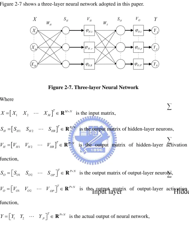
Figure 2-7 shows a three-layer neural network adopted in this paper.
Figure 2-7. Three-layer Neural Network
Where
[
1 2]
T M N
M
X = X X X ∈ R ×
L is the input matrix,
[
1 2]
T R N
H H H HR
S = S S S ∈ R ×
L is the output matrix of hidden-layer neurons,
[
1 2]
T R N
H H H HR
V = V V V ∈ R ×
L is the output matrix of hidden-layer activation function,
1 2
T P N
O O O OP
S =⎡⎣S S L S ⎤⎦ ∈R × is the output matrix of output-layer neurons,
1 2
T P N
O O O OP
V =⎡⎣V V L V ⎤⎦ ∈R × is the output matrix of output-layer activation function,
1 2
T P N
P
Y =⎡Y Y Y ⎤ ∈ ×
⎣ L ⎦ R is the actual output of neural network,
And N denotes the number of training data. M, R and P denote the number of input neurons, hidden-layer neurons and output-layer neurons, respectively. Further we define the weighting matrices:
,1 H ϕ , H r ϕ , H R ϕ ,1 O ϕ , O P ϕ , O p ϕ H V X SH SO VO Y 1 X m X M X 1 Y p Y P Y Y W H W
(1,1) (1, ) ( ,1) ( , ) H H M H H R H R M R M W W W W W × ⎡ ⎤ ⎢ ⎥ ⎢ ⎥ =⎢ ⎥ ⎢ ⎥ ⎢ ⎥ ⎣ ⎦ L L M O M M O M L L (2.37) (1,1) (1, ) ( ,1) ( , ) Y Y R Y Y P Y P R P R W W W W W × ⎡ ⎤ ⎢ ⎥ ⎢ ⎥ =⎢ ⎥ ⎢ ⎥ ⎢ ⎥ ⎣ ⎦ L L M O M M O M L L (2.38) Where: ( , ) H r m
W denotes weight value between the mth neuron in the input layer and rth neuron in the hidden layer.
( , )
Y p r
W denotes weight value between the rth neuron in the hidden layer and pth neuron in the output layer.
And ( )ϕH x is the activation function of the hidden layer. ϕO( )x is the activation function of the output layer. Usually, we both use the same sigmoid function for them. So we have 1 ( ) ( ) 1 H x O x e x ϕ =ϕ = − + (2.39)
2.5.2 Updating Process of a Three Layer Neural Network
Let 1 2
T P N
P
D=⎡⎣D D L D ⎤⎦ ∈R × represents the desired output matrix and E denotes the error matrix and cost function J represents a normalized total square error function with η stands for the learning rate parameter in back-propagation algorithm. Based on BAP, the training process includes the following forward and backward passes:
(1) Forward pass (computing cost function):
H H R N
S =W X × ; VH =ϕH(SH) R N× ; SO =W VY H P N× ; Y V= O =ϕO(SO) P N×
P N
E Y D= − × ;
The normalized total square error function is defined as:
(
( , ) ( , ))
2(
)
1 1 1 1 trace 2 2 P N p n p n p n J Y D EE PN = = PN ′ =∑∑
− = (2.40)(2) Backward pass (update rule of synaptic weights):
(t 1) ( )t ( )t ( )t t J W W W W W η + ∂ = − ∆ = − ∂ (2.41) ( , ) ( , ) ( ,:) ( ,:) ( ,:) ( ,:) ( ,:) ( 1) ( ) 1 ( ) (1 ) p r p r p p p p r Y t Y t O O O H W W V D V V V PN η + = − − − (2.42)
(
)
(
)
( , ) ( , ) ( ,:) ( ,:) ( ,:) ( ,:) ( , ) ( ,:) ( ,:) ( ,:) ( 1) ( ) 1 1 (1 ) 1 P r m r m p p p p p r r r m H t H t O O O Y H H p W W V D V V W V V X PN η + = ⎛ ⎞ = − ⎜ − − ⎟ − ⎝∑
⎠ (2.43)2.5.3 Dynamical Optimal Training via Lyapunov’s Method
We define the Lyapunov function as:
V = J
The item J is normalized total square error, defined in (2.40). Now if we consider learning rate η as a variable, then J(η) denotes a positive function of η. We use WY(t+1)
and WH(t+1) to compute the normalized total square error of iteration t+1: Jt+1. And we
can define the difference of the Lyapunov function as: ( , )t ( , t 1) ( , )t
V Jη Jη + Jη
∆ = ∆ = −
So if we can find a learning rate η to make both ΔJ(η ,t) < 0 and ΔJ(η ,t) be at its minimum then we can get a stable and optimal convergence network. By using (2.40) we can get
(
( , ) ( , ))
2(
( , ) ( , ))
2 1 1 1 1 1 1 1 1 2 2 P N P N p n p n p n p n t t t t p n p n J J Y D Y D PN PN + + = = = = − =∑∑
− −∑∑
− (2.41)(
( , ) ( , )) (
2 ( , ) ( , ))
2 1 1 1 1 2 P N p n p n p n p n t t p n Y D Y D PN = = + ⎡ ⎤ = ⎢ − − − ⎥ ⎣ ⎦∑∑
(
( ))
G η t = (2.42) From (2.42), if the parameter η(t) satisfies Jt+1 - Jt = G(η(t)) <0, then η(t) is the stablelearning rate of the system at the tth iteration. For stable η(t), if the ηopt(t) will let that Jt+1
- Jt be at its minimum, the ηopt(t) is the optimal learning rate at the tth iteration. The
optimal learning rate ηopt(t) will not only guarantee the stability of the training process,
but it also has the fastest speed of convergence.
How to find the optimal learning rate ηopt(t) from G(η(t))? Because G(η(t)) is a very
complicated nonlinear algebraic function, it is hard to have a well designed formula for finding the optimal learning rate ηopt(t) from G(η(t)). Hence, we use the MATLAB
routine “fminbnd” to search the optimal learning rate from (2.41).The calling sequence of “fminbnd” is [27]:
FMINBND Scalar bounded nonlinear function minimization.
X = FMINBND(FUN,x1,x2) starts at X0 and finds a local minimizer X of the function FUN in the interval x1 <= X <= x2. FUN accepts scalar input X and returns a scalar function value F evaluated at X.
The capability of the Matlab routine “fminbnd” is to find a local minimizer ηopt of the
function G(η), which has only one independent variable η, in a given interval. So we have to define an interval when we use this routine.
Algorithm 1:
Dynamic optimal training algorithm of a Three Layer Neural Network [19] Step 0: Give input matrix X and desired output matrix D.
Step 1: Set initial weight factor WH and WY, which are random values in a small random
range. Set maximum acceptable final value of the cost function J0. Step 2: Iteration count k=1.
Step 3: Start forward pass of back-propagation training process.
Step 4: Compute error function E(k)=Y(k)-D(k) and cost function J(k). If J(k) is smaller
than acceptable value J0 , the algorithm goes to Step 8. If no, it goes to Step 5. Step 5: Using Matlab routine “fminbnd” with the search interval [0.01, 100] to solve the
nonlinear function ∆J(k)=J(k+1)-J(k) and find the optimal learning rate ηopt(t). Step 6: Start backward pass of back-propagation training process. Update the synaptic
weights matrix to yield WH(k+1) and WY(k+1) by using (2.42) and (2.43)
respectively.
Step 7: Iteration count k=k+1, and algorithm goes back to Step 3. Step 8: End the algorithm.
CHAPTER 3
Dynamic Optimal Training Algorithm of A Three-Layer
Neural Network with Better Performance
The structure of three layer neural network was presented in Chapter 2 with preparation for its improved dynamical optimal training to be presented in this Chapter 3. Although the dynamical optimal training of a three layer neural network was presented in [19], its back propagation algorithm with dynamical optimal learning rates can not guarantee global convergence. Although we can decrease the learning rate to have a better chance of global convergence, its convergence speed will be really slow. Also, the sigmoid function adopted for the activation functions for each layer will also slow down the training process. Therefore the following approaches will be proposed to further improve the performance of the dynamical optimal training of a three layer neural network. They are:
1. Simplification of activation function: Replace the sigmoid activation function in the second (output) layer with a linear activation function. (Section 3.2)
2. Selection of proper initial weighting factors: By confining the initial
weighting matrices in a reasonable range, the training process can have a better chance to reach global convergence. (Section 3.3)
3. Determine the upper-bound of learning rate in each iteration: Therefore the
search of optimal learning rate in each iteration can be simplified to increase the speed of convergence. (Section 3.4)
3.1 Problems in the Training of Three Layer Neural Network
There are two layers of sigmoid activation functions in Fig. 2-6, i.e., VH and VO for hidden and output layers. The purpose of activation function is to confine the output in each layer to a proper level. But the computing effort in computing the sigmoid function is much more than that in computing a linear function. Further it may be good enough to confine the output of hidden layer to a reasonable level. Once the data flow thru the output layer, the chance of the output data to lie outside proper level is small. These observations lead us to simplify the activation function in the output layer so that the speed of training process can be increased. Considering the defects of sigmoid function, whose graph is s-shaped, as shown below (Figure 3-1) with
1 1 exp( ) y ax = + − (3.1) where y is the output signal of the neuron and x is the input signal. And the parameter a is the slope parameter of the sigmoid function. We can get different sigmoid functions by varying the slope parameter a, but we usually choose the sigmoid function with a =1.
-10 -8 -6 -4 -2 0 2 4 6 8 10 0 0.1 0.2 0.3 0.4 0.5 0.6 0.7 0.8 0.9 1 X y= V o Sigmoid Function
When x is far away from 0, we will get a saturated output value which is very close to extreme value, i.e., 0 or 1. Now we will discuss the problem which is caused by this saturation. First consider (2.42), which is update rule of weighting factors in output layer ( , ) ( , ) ( ,:) ( ,:) ( ,:) ( ,:) ( ,:) ( 1) ( ) 1 ( ) (1 ) p r p r p p p p r Y t Y t O O O H W W V D V V V PN η + = − − −
We define the error signal of the weight between pth output layer neuron and rth hidden layer neuron as ( , )
1
( ,:) ( ,:) ( ,:) ( ,:)(
)
(1
)
p r p p p r OV
OD V
OV
OV
HPN
δ
=
−
−
(3.2) So (2.42) can be rewritten as ( , ) ( , ) ( , ) ( 1) ( ) p r p r p r Y t Y t O W + =W −ηδ (3.3)Consider (2.43), which is update rule of weighting factors in hidden layer
(
)
(
)
( , ) ( , ) ( ,:) ( ,:) ( ,:) ( ,:) ( , ) ( ,:) ( ,:) ( ,:) ( 1) ( ) 1 1 (1 ) 1 P r m r m p p p p p r r r m H t H t O O O Y H H p W W V D V V W V V X PN η + = ⎛ ⎞ = − ⎜ − − ⎟ − ⎝∑
⎠For simplicity, we define a new error signal as
(
)
( , ) 1 ( ,:) ( ,:) ( ,:) ( ,:) (1 ) p r p p p p H VO D VO VO PN δ = − − (3.4) and the error signal of the weight between rth hidden layer neuron and mth input layer neuron as(
)
( , ) ( , ) ( , ) ( ,:) ( ,:) ( ,:) 1 1 P r m p r p r r r m H H Y H H p W V V X δ δ = ⎛ ⎞ =⎜ ⎟ − ⎝∑
⎠ (3.5)So, (2.43) can be rewritten as
( , ) ( , ) ( , ) ( 1) ( )
r m r m r m
H t H t H
W + =W −ηδ (3.6)
In (3.2) & (3.4) the term VO(p,n)(1-VO(p,n)) will propagate back to the hidden and input
layers to adjust weighting factors. The term VO(p,n)(1-VO(p,n)) will be very small if VO(p,n)
case, the back-propagated error signal δO(p,r) will not actually reflect the true error
VO(p,n)-D = Y-D. This will lead to local minima problem. Note that the term
VO(p,n)(1-VO(p,n)) is originated from the derivative of the sigmoid activation function. So
it is important not to let the term VO(p,n)(1-VO(p,n)) closed to 0 or 1 in the beginning phase
of training. Therefore the initial weighting factors must be carefully chosen. Further the sigmoid function may not be a good choice for the sake of computation effort and the above mentioned problem. Thus the search for a better and yet simplified activation function with the selection of proper initial weighting factors will be mentioned in 3.2 and 3.3.
3.2 Simplification of activation function
We define the linear function (without saturation) as ( )
O x ax
ϕ =
where a is an adjustable parameter which means slope of the function. The reason of using an unbounded linear function in stead of a saturated one can be found in Appendix A. Usually, we set parametera=1.With the replacement of the sigmoid activation function by a linear activation function, we can redefine the new error signal of the weight between pth output layer neuron and rth hidden layer neuron. Consider (2.41), which is the update rule of weighting factors for BP algorithm
( ,:) ( ,:) ( , ) ( , ) ( , ) ( 1) ( ) ( , ) ( ) ( ,:) ( ,:) ( , ) p p p r p r p r O O Y t Y t p r Y t p p p r Y O O Y V S J J W W W W V S W η η + ∂ ∂ ∂ ∂ = − = − ∂ ∂ ∂ ∂ (3.7)
If ( )ϕO x =ax , then the term∂VO( ,:)p ∂SO( ,:)p will be equal to a. So ∂ ∂J VO( ,:)p , ( ,:)p ( ,:)p
O O
V S
∂ ∂ , and ∂SO( ,:)p ∂WY( ,:)p have new presentations as
(
( ,:) ( ,:))
2(
( ,:) ( ,:))
1 P p p 1 p p J V D V D ⎛ ⎞ ∂ = ∂ − = − ⎜∑
⎟ (3.8)( ,:) ( , ) ( ,:) ( ,:) ( , ) ( , ) 1 p R p r r r O Y H H p r p r r Y Y S W V V W W = ∂ = ∂ ⎛ ⎞= ⎜ ⎟ ∂ ∂ ⎝
∑
⎠ (3.9)(
)
( ,:) ( ,:) ( ,:) ( ,:) p p O O p p O O V aS a S S ∂ ∂ = = ∂ ∂ (3.10)From previous three equations, we can rewrite the update rule of weighting factors in output layer as ( , ) ( , ) ( ,:) ( ,:) ( ,:) ( 1) ( ) ( ) p r p r p p r Y t Y t O H a W W V D V PN η + = − − (3.11) And update rule of weighting factors in hidden layer can be expressed as
(
)
(
)
( , ) ( , ) ( ,:) ( ,:) ( , ) ( ,:) ( ,:) ( ,:) ( 1) ( ) 1 1 P r m r m p p p r r r m H t H t O Y H H p a W W V D W V V X PN η + = ⎛ ⎞ = − ⎜ − ⎟ − ⎝∑
⎠ (3.12)Hence, the error signals δO( , )p r and δH( , )r m become
( , ) ( ,:) ( ,:)
(
)
p r p r O O Ha
V
D V
PN
δ
=
−
(3.13)(
)
(
)
( , ) ( ,:) ( ,:) ( , ) ( ,:) ( ,:) ( ,:) 1 1 P r m p p p r r r m H O Y H H p a V D W V V X PN δ = ⎛ ⎞ =⎜ − ⎟ − ⎝∑
⎠ (3.14)We can see that the error signal δO( , )p r in (3.13) will not be discounted by the term
VO(p,n)(1-VO(p,n)), like that in (2.42) (or (3.3)). This will remove the effect of improper
initial weighting factors to let the term VO(p,n)(1-VO(p,n)) close to 0 or 1 in the beginning
phase of training. From (3.14), although the term VO(p,n)(1-VO(p,n)) is also eliminated
(from (3.4)), we still have the similar term VH(r,n)(1-VH(r,n)) in (3.14). Therefore we
should do is to confine the selection of initial weighting factors in a proper range so that the term VH(r,n)(1-VH(r,n)) will not be closed to 1 or 0 in the beginning phase of training.
The reason why we can not replace the sigmoid activation function in the hidden layer with the similar linear activation function can be shown in Appendix B.
3.3 Selection of Initial Weighting Factors
(
( ,:) ( ,:))
( , ) 1 P p p p r H O Y p a V D W PN δ = ⎛ ⎞ =⎜ − ⎟ ⎝∑
⎠ % (3.15)So (3.14), which is the new error signal in hidden layer, can be rewritten as
(
)
( , ) ( ,:) ( ,:) ( ,:) 1 r m r r m H H HV VH X δ =δ% − (3.16)It can be found that the term VH(r,n)(1-VH(r,n)) still causes the saturation problem. When VH(r,n) closes to 0 or 1, the term VH(r,n)(1-VH(r,n)) will discount back-propagated real error
signal (3.15). In (3.16), the term VH(r,n) is the output of sigmoid activation function, and
it is a function of initial weighting factors. If we can confine VH(r,n) in the range of, say
[0.2, 0.8], then the term (1-VH(r,n)) in (3.16) will also be confined in the range of [0.2,
0.8]. Therefore the whole term VH(r,n)(1-VH(r,n)) in (3.16) will not close to zero if proper
initial weighting factors are selected. This will prevent the error signal of hidden layer in (3.16) be discounted by the whole term VH(r,n)(1-VH(r,n)) in the beginning phase of
training. The VH(r,n) can be expressed as
( , ) ( , ) ( ,:) 1 1 exp r n j i i H h h i V = ⎛⎜ + ⎛⎜− W X ⎞⎟⎞⎟ ⎝ ⎠ ⎝
∑
⎠ (3.17)where Xhi is the fixed input data. To decrease the effect of saturation region, we can
choose proper initial weighting factors so that the term VH(r,n) will locate in the range of
[0.2, 0.8] at the beginning of training process.
It is a normal practice to use random number generator to select the initial weighting factors. Let max min ( ) ( ) w Max W w Min W = =
Where W is the weighting matrix. It is also shown in [17] that the training of NN will have better convergence if the mean of random initial weighting factors is zero. Therefore we let w < <0 w and w = −w . We use a sigmoid activation
function with parameter a = 1 in hidden layer. Then we must select w and min wmax to satisfy the following inequality:
min max
0.2
=
y w
s(
, )
λ
≤
y w
s( , )
λ
≤
y w
s(
, ) 0.8
λ
=
(3.18) with s 1 y ( , ) 1 exp( ) w w λ λ = + − (3.19) We let λ= xmax in the following Theorem 1, where xmax is the maximum absolute value of the elements of input matrix and wmin ≤ ≤w wmax. From (3.18), we can havemax max max min max ln 4 ln 4 ln 4 w x w x w x ⎧ = ⎪ ⎪ ⇒ ≤ ⎨ − ⎪ = ⎪⎩ (3.20) Theorem 1:
If w satisfies (3.20), then the output of sigmoid function in (3.19), i.e.,y w xs( , max), will
be in the range of [0.2, 0.8]. Proof:
Know that wmin ≤ ≤w wmax
∵ y ws
(
,λ)
is a strictly increasing function so if wλ≤wλ⇒ y ws( )
λ ≤ y ws( )
λ ∴ y ws(
min, xmax)
≤ y w xs(
, max)
≤ y ws(
max, xmax)
∵ min max ln 4 w x = − and max max ln 4 w x =
∴
(
)
(
)
min max max max max max max max 1 , 0.2 ln 4 1 exp( ( )) 1 , 0.8 ln 4 1 exp( ) s s y w x x x y w x x x = = + − − = = + −∴ 0.2= y ws
(
min, xmax)
≤ y w xs(
, max)
≤y ws(
max,xmax)
=0.8(
max)
0.2 y w xs , 0.8
⇒ ≤ ≤
Q.E.D.
Theorem 2:
If 0.2≤ y w xs( , max )≤0.8, then 0.2≤ y w xs( , i)≤0.8. Here y w xs( , max) & y w xs( , i)
are defined in (3.19) and w is selected from (3.20). Proof: (1) For w > 0 ∵ 0≤w xi ≤w xmax ∴ 0.5= y ws
(
, 0)
≤ y w xs(
, i)
≤y w xs(
, max)
∴ y w xs(
, i)
≥0.5 ∵ y w xs(
, max)
≤0.8 ∴ 0.5≤ y w xs(
, i)
≤0.8 ⇒ 0.2< y w xs(
, i)
≤0.8……(a) (2) For w < 0 ∵ w xmax ≤w xi ≤0 ∴ y w xs(
, max)
≤ y w xs(
, i)
≤ y ws(
, 0)
=0.5 ∴ y w xs(
, i)
≤0.5(
)
∴ 0.2≤ y w xs
(
, i)
≤0.5 ⇒ 0.2≤ y w xs(
, i)
<0.8……(b) From (a) and (b), we have the final conclusion0.2≤y w xs( , i )≤0.8
Q.E.D.
Theorem 3:
If 0.2≤ y w xs( , i)≤0.8, then 0.2≤ y w xs( , )i ≤0.8. Here w is selected from (3.20).
Proof: (1) 0xi > ∵ y w xs( , i)= y w xs( , )i ∴ 0.2≤ y w xs( , i)= y w xs( , )i ≤0.8 ⇒ 0.2≤ y w xs( , )i ≤0.8 (2) 0xi < ∵ y w xs( , )i = y ws( ,− xi) ⇒
(
,)
1 1(
,)
1 exp( ( )) 1 exp( ( ) ) s i s i i i y w x y w x w x w x − = = = − + − − + − − ⇒ ys(
−w x, i)
=y w xs(
%, i)
∴ y w xs( , )i = y w xs( ,% i)From Theorem 2, we have 0.2≤y w xs
(
%, i)
≤0.8 ∴ 0.2≤ y w xs( , )i ≤0.8Q.E.D.
The above Theorem 3 is our final conclusion, which selects proper weighting factors to
let 0.2 ( , ) 1 0.8 1 exp( ) s i i y w x wx ≤ = ≤
+ − , so that the error signal (3.16) in hidden layer will not be discounted in the beginning of training process. This will also reduce the
probability of falling into in local minimum on the error surface during the back propagation process.
Example 3-1: Selection of Initial Weighting Factors
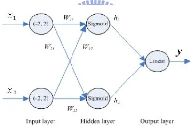
Give the following neural network with three layers, two inputs in the input layer, one output neuron in the output layer, and two neurons in the hidden layer. It adopts sigmoid function as hidden layer activation function, and the above mentioned linear function as output layer activation function. The input signals are bound at (-2, 2). The architecture of the neural network is shown in Figure 3-2. Find the initial weighting factors so that the initial outputs of the sigmoid functions in the hidden layer will be in the range of [0.2, 0.8].
Figure 3-2. Neural Network for Example 3-1 Solution:
Since xmax = , from (3.19) we can get: 2 min max ln 4 ln 4 ln 4 0.6931 2 2 w x − − − = = = = − and max max ln 4 ln 4 ln 4 0.6931 2 2 w x = = = =
Hence, the range of initial weight factors is [-0.6931, 0.6931]. For verification, we assume four different input pair [x1, x2] and randomly choose four initial weighting factors [w11, w12, w21, w22] = [-0.22669, -0.15842, 0.33254, -0.17167] from [-0.6931,
Table 3-1 Output of Sigmoid function in hidden layer
x1 -0.01 0.7 -1.91 0.67
x2 1.2 2 -1.5 0.34
h1 0.45318 0.38331 0.66164 0.44874
h2 0.44786 0.47239 0.40670 0.54102
From Table 3-1, we can find that for every input pair [x1, x2], the initial outputs of
hidden neurons [h1, h2] are all in the range of [0.2, 0.8].
END
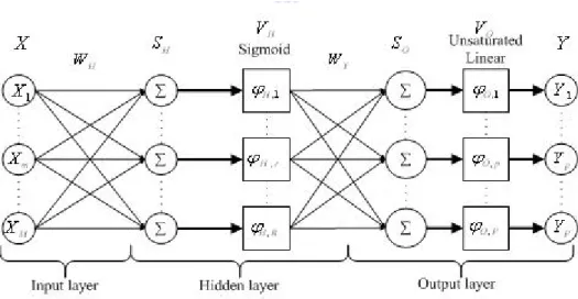
To summarize the above proposed issues, the following Figure 3-3 shows the modified three-layer NN proposed in this Chapter 3.
Figure 3-3. Revised Three Layer Neural Network
3.4 Determine the upper-bound of learning rate in each iteration
In the dynamic optimal training algorithm, we use matlab function “fminbnd” to find optimal learning rate. The calling sequence of “fminbnd” is [27]:
FMINBND Scalar bounded nonlinear function minimization.