多天線隨意無線系統的統計通道模型之研究

全文

(1)國立交通大學電信工程學系碩士論文多天線隨意無線系統的統計通道模型之研究 Statistical MIMO Channel Models for Mobile-to-Mobile Ad Hoc Communication Systems. 研究生：鄭允懷指導教授：王蒞君中. 華. 民. 國. 九十四. 年. 十. 月.

(2) Statistical MIMO Channel Models for Mobile-to-Mobile Ad Hoc Communication Systems. A THESIS Presented to The Academic Faculty By Yun-Huai Cheng In Partial Fulfillment of the Requirements for the Degree of Master in Communication Engineering Department of Communication Engineering National Chiao-Tung University. October, 2005 c Copyright °2005 by Yun-Huai Cheng.

(3) 摘要在智慧型運輸系統及隨意網路的應用下，移動通訊 (mobile-to-mobile)是一個非常重要的元素。在此種系統下，傳送及接收兩端皆同時處在移動狀態之下，且同時受到散射(Scattering) 與萊斯衰變(Rician fading)的影響。因此在本篇論文裡，我們將會提出一個具相關性的雙環散射模型(correlated double-ring)以及正弦函數累加的模擬方法(sum-of-sinusoids simulation method) 來描述在傳收兩端間具有直視能量(line-of-sight)下的移動通訊系統之通道模型(mobile-to-mobile Rician fading channel model)。我們所提出的模型將可應用在隨意通訊系統的物理層模擬。隨著現代通訊系統對通道容量(capacity)的需求增加，把多根天線(MIMO)的技術應用在移動通訊系統上的方法，已逐漸受到軍事及商業上的重視。就如同在傳統的蜂巢式通訊網路(cellular network) 下，多天線技術可以提供媒體存取控制(MAC)協定設計時的空間 (spatial)自由度一樣，在隨意網路下我們也可以藉由多天線的技術來提供足夠的多樣性與通道容量。不過，在多天線隨意網路下如何能夠準確的模擬出空間及時間的通道相關性(spatial/temporal channel correlation)對移動通訊環境的影響，是一個重要且基本的問題。在此種多天線系統的通道中，.

(4) 傳收兩端間直視的能量以及不同的散射環境將會對通道容量與通道容量的平均衰變時間(average fade duration)有所影響。在此篇論文中，我們以所提出的相關性雙環散射模型為基礎，建立一個以正弦函數累加方法所構成的移動性多天線通道模型(mobile-to-mobile MIMO)，此模型將可以精確的描述出空間的相關性、時間的相關性與萊斯參數對通道衰變的影響。我們最後則觀察多天線系統的通道容量其衰變情形和萊斯參數之間的關係。.

(5) Summary Mobile to mobile communication is one of important applications for the intelligent transport systems and mobile ad hoc networks. In such a system, both the transmitter and receiver are in motion, of which the signals experience Rician fading and different scattering effects. In this thesis, we present a correlated double-ring scattering model and a sum-of-sinusoids simulation method to characterize such a mobile-to-mobile Rician fading channel. The developed model can facilitate the physical layer simulation of a mobile ad hoc communication system. With the increasing of the demand on channel capacity in modern communications, multiple-input Multiple-output (MIMO) mobile ad hoc networks have been receiving increasingly attention in both commercial and military applications. Just as in cellular networks, MIMO technology can benefit ad-hoc networks by providing the diversity and capacity advantages as well as the spatial degree of freedom in designing the media access control (MAC) protocol. However, one fundamental issue to MIMO mobile ad-hoc networks is how to accurately model the impact of spatial/temporal channel correlation in mobile-to-mobile communication environment. In such a channel, a line-of-sight (LOS) component and different scattering environments will affect both ergodic capacity and average capacity fade duration of the MIMO system. In this thesis, based on the correlated double-ring scattering model we have also suggest a sum-of-sinusoids MIMO mobile-to-mobile channel simulation method, which can characterize the spatial/temporal channel correlation and Rician fading effect. We investigate how often the MIMO capacity experience the fades and relate this to the Rician factor..

(6) Acknowledgments. I would like to thank my family who always give me supports and endless love. I especially would like to appreciate Dr. Li-Chun Wang who gave me many valuable suggestions and guidance in the research. I would not finish this work without his encouragement, comments, and advice. In addition, I deeply grateful to my laboratory mates, Chiung-Jang, Ming-Bing, Chih-Wen, Wei-Cheng, Chang-Lung, Chung-Wei, Lei, Wei-Jun, Yi-Cheng, ChingHau, Kuang-Nan, Assane, Chu-Jung, Cheng-Wei and Hung-Hsi at WNLAB at the Department of Communications in National Chiao-Tung University. They provide me much assistance and share much happiness with me.. vi.

(7) vii. Contents. Summary. v. Acknowledgements. vi. List of Figures. x. 1 Introduction. 1. 1.1. Problem and Solution . . . . . . . . . . . . . . . . . . . . . . . . . . .. 3. 1.1.1. Mobile-to-Mobile Rician Fading Channel Model . . . . . . . .. 4. 1.1.2. Average Fade Duration of Mobile-to-Mobile Rician Fading Channels . . . . . . . . . . . . . . . . . . . . . . . . . . . . . . . . .. 1.1.3. Capacity Analysis of MIMO Mobile-to-Mobile Rician Fading Channels . . . . . . . . . . . . . . . . . . . . . . . . . . . . . .. 1.1.4. 1.2. 4. 5. Higher Order Statistics of Mobile-to-Mobile MIMO Rician Channels . . . . . . . . . . . . . . . . . . . . . . . . . . . . . . . . .. 5. Thesis Outline . . . . . . . . . . . . . . . . . . . . . . . . . . . . . . .. 6. 2 Background. 7. 2.1. Discrete Line Spectrum Method . . . . . . . . . . . . . . . . . . . . .. 7. 2.2. Inverse Discrete Fourier Transform Method . . . . . . . . . . . . . . .. 8. 2.2.1. Smith’s Method . . . . . . . . . . . . . . . . . . . . . . . . . .. 8. 2.2.2. Young and Beaulieu’s Method . . . . . . . . . . . . . . . . . .. 10. Sum-of-Sinusoids Approximation Method . . . . . . . . . . . . . . . .. 10. 2.3.

(8) 3 Mobile-to-Mobile Rician Fading Channel Model. 12. 3.1. Introduction . . . . . . . . . . . . . . . . . . . . . . . . . . . . . . . .. 12. 3.2. Scattering Environment . . . . . . . . . . . . . . . . . . . . . . . . .. 14. 3.2.1. Traditional Double-Ring Scattering Model . . . . . . . . . . .. 14. 3.2.2. Correlated Double-Ring Scattering Model . . . . . . . . . . .. 15. Sum-of-Sinusoids Rician Fading Simulator . . . . . . . . . . . . . . .. 16. 3.3.1. Signal Model based on Correlated Double-Ring Scattering . .. 16. 3.3.2. Second-Order Statistics . . . . . . . . . . . . . . . . . . . . . .. 17. 3.3.3. Signal Model Based on Single-Ring Scattering . . . . . . . . .. 18. Numerical Results . . . . . . . . . . . . . . . . . . . . . . . . . . . . .. 19. 3.4.1. Effects of Numbers of Scatterers . . . . . . . . . . . . . . . . .. 19. 3.4.2. Effects of Rician Factor . . . . . . . . . . . . . . . . . . . . . .. 20. 3.4.3. Comparison of Correlated Double-Ring and Single-Ring Models 21. 3.3. 3.4. 3.5. Conclusions . . . . . . . . . . . . . . . . . . . . . . . . . . . . . . . .. 21. 4 Average Fade Duration of Mobile-to-Mobile Rician Fading Channels 32 4.1. Introduction . . . . . . . . . . . . . . . . . . . . . . . . . . . . . . . .. 32. 4.2. Higher-Order Statistics . . . . . . . . . . . . . . . . . . . . . . . . . .. 33. 4.2.1. Level-Crossing Rate . . . . . . . . . . . . . . . . . . . . . . . .. 33. 4.2.2. Average Fade Duration . . . . . . . . . . . . . . . . . . . . . .. 35. 4.3. Numerical Results . . . . . . . . . . . . . . . . . . . . . . . . . . . . .. 35. 4.4. Conclusions . . . . . . . . . . . . . . . . . . . . . . . . . . . . . . . .. 36. 5 Capacity Analysis of MIMO Mobile-to-Mobile Rician Fading Channels. 39. 5.1. Introduction . . . . . . . . . . . . . . . . . . . . . . . . . . . . . . . .. 39. 5.2. Scattering Model . . . . . . . . . . . . . . . . . . . . . . . . . . . . .. 41. 5.3. Sum-of-Sinusoids MIMO Rician Fading Simulator . . . . . . . . . . .. 42. 5.3.1. 42. Line-of-sight Component Model . . . . . . . . . . . . . . . . .. viii.

(9) 5.3.2. Sum-of-Sinusoids Simulation Method . . . . . . . . . . . . . .. 44. 5.4. Capacity Evaluation . . . . . . . . . . . . . . . . . . . . . . . . . . .. 46. 5.5. Numerical Results . . . . . . . . . . . . . . . . . . . . . . . . . . . . .. 48. 5.5.1. Ergodicity . . . . . . . . . . . . . . . . . . . . . . . . . . . . .. 49. 5.5.2. Impacts of Doppler Frequencies . . . . . . . . . . . . . . . . .. 50. 5.5.3. Effect of Spatial Correlation . . . . . . . . . . . . . . . . . . .. 51. 5.5.4. Impact of Numbers of Antennas . . . . . . . . . . . . . . . . .. 52. 5.5.5. Impact of Numbers of Scatterers. . . . . . . . . . . . . . . . .. 52. Conclusions . . . . . . . . . . . . . . . . . . . . . . . . . . . . . . . .. 53. 5.6. 6 Higher Order Statistics of Mobile-to-Mobile MIMO Rician Channels. 55. 6.1. Introduction . . . . . . . . . . . . . . . . . . . . . . . . . . . . . . . .. 55. 6.2. Level Crossing Rate and Average Fade Duration . . . . . . . . . . . .. 55. 6.3. Numerical Results . . . . . . . . . . . . . . . . . . . . . . . . . . . . .. 57. 6.3.1. Capacity Distribution . . . . . . . . . . . . . . . . . . . . . . .. 57. 6.3.2. LCR and AFD . . . . . . . . . . . . . . . . . . . . . . . . . .. 58. Conclusions . . . . . . . . . . . . . . . . . . . . . . . . . . . . . . . .. 58. 6.4. 7 Concluding Remarks. 63. 7.1. Mobile-to-Mobile Rician Fading Channel Model . . . . . . . . . . . .. 64. 7.2. Average Fade Duration of Mobile-to-Mobile Rician Fading Channels .. 64. 7.3. Capacity Analysis of MIMO Mobile-to-Mobile Rician Fading Channels. 65. 7.4. Higher Order Statistics of Mobile-to-Mobile MIMO Rician Channels .. 65. 7.5. Suggestion for Future Work . . . . . . . . . . . . . . . . . . . . . . .. 66. Bibliography. 67. Vita. 70. ix.

(10) x. List of Figures 2.1. Block diagram of the algorithm of Smith to generate correlated Rayleigh variates. . . . . . . . . . . . . . . . . . . . . . . . . . . . . . . . . . .. 2.2. Block diagram of the improved algorithm using a single complex IDFT to generate correlated Rayleigh variates. . . . . . . . . . . . . . . . .. 3.1. 24. Relative velocity V3 from the TX with velocity V1 to the RX with velocity V2 . . . . . . . . . . . . . . . . . . . . . . . . . . . . . . . . .. 3.4. 23. Scattering environment in a mobile-to-mobile system with a LOS component. . . . . . . . . . . . . . . . . . . . . . . . . . . . . . . . . . . .. 3.3. 10. The independent two-ring scattering model for the mobile-to-mobile Rayleigh fading channel. . . . . . . . . . . . . . . . . . . . . . . . . .. 3.2. 9. 25. Single-ring scattering environment for a mobile-to-mobile Rician fading channel. . . . . . . . . . . . . . . . . . . . . . . . . . . . . . . . . . .. 26. 3.5. The autocorrelation function of the complex envelope Z(t), where K = 1. 27. 3.6. The autocorrelation function of the complex envelope Z(t), where N = M = 8 for K = 0, 1, 3, and 9.. . . . . . . . . . . . . . . . . . . . . . .. 28. 3.7. The PDF of the fading envelope Z(t) when N = M = 8. . . . . . . .. 29. 3.8. The real part of the fading envelope of double-ring and single-ring scattering models. . . . . . . . . . . . . . . . . . . . . . . . . . . . . .. 3.9. 30. The difference of the real part of the fading envelope Z(t) based on the double-ring scattering model from that based on the single-ring scattering model when K varies from 0.1 to 20. . . . . . . . . . . . .. 31.

(11) 4.1. Normalized envelope level crossing rate for mobile-to-mobile Rician fading. Solid line denotes the theoretical results and the dashed line denotes the simulation results, where ρ = √R . . . . . . . . . . . . . . Ωp. 4.2. 37. Normalized average fade duration for a mobile-to-mobile Rician fading channel for K = 10, 7, 3, and 1. . . . . . . . . . . . . . . . . . . . . .. 38. 5.1. Correlated double-ring scattering model with LOS components. . . .. 42. 5.2. Received signals at multiple antennas with an AOA θrn and separation distance d under the assumption that the transmission distance is much longer than d. . . . . . . . . . . . . . . . . . . . . . . . . . . . . . . .. 5.3. LOS component model for moving transmitter TX and receiver RX of which vectors are V1 and V2 with a relative angle of θβ , respectively. .. 5.4. 53. MIMO Rician Capacity with different Doppler frequencies where SNR = 20 dB, d = λ/2 ,K = 3. . . . . . . . . . . . . . . . . . . . . . . . . . .. 6.2. 52. The ergodic capacity of MIMO channels against the number of antennas when SNR = 20 dB, d = λ/2 and K = 0. . . . . . . . . . . . . . .. 6.1. 51. Capacity per antenna against the number of antennas when SNR = 20 dB, d = λ/2. . . . . . . . . . . . . . . . . . . . . . . . . . . . . . . . .. 5.9. 50. The ergodic capacity of MIMO channles against the number of antennas when SNR = 20 dB, and d = λ/2. . . . . . . . . . . . . . . . . . .. 5.8. 49. Effect of antenna separation on the ergodic capacity of a 3 × 3 MIMO channel for SNR = 20 dB and various values of K factors. . . . . . .. 5.7. 48. MIMO Rician Capacity with different Doppler frequencies where SNR = 20 dB, d = λ/2 ,K = 3. . . . . . . . . . . . . . . . . . . . . . . . . . .. 5.6. 45. The time and the ensamble average capacity outage probability of a 3 × 3 MIMO channel when K = 3, SNR = 20 dB, and d = λ/2. . . .. 5.5. 43. 59. Probability density functions of MIMO capacity in a mobile-to-mobile Rician fading channel. . . . . . . . . . . . . . . . . . . . . . . . . . .. xi. 60.

(12) 6.3. Level crossing rate of the MIMO capacity in a mobile-to-mobile Rician fading channel. . . . . . . . . . . . . . . . . . . . . . . . . . . . . . .. 6.4. 61. Average fade duration of the MIMO capacity in a mobile-to-mobile Rician fading channel. . . . . . . . . . . . . . . . . . . . . . . . . . .. xii. 62.

(13) 0.

(14) 1. CHAPTER 1 Introduction Mobility affects wireless networks significantly. In traditional cellular systems, the base station is stationary and only mobile terminals are in motion. However, in many new wireless system, such as the intelligent transport systems (ITS) and mobile ad hoc networks, a mobile directly connects to another mobile without the help of fixed base stations. Thus, how mobility affects a system where both the transmitter and the receiver move simultaneously becomes an interesting problem. From the propagation perspective, the scattering environment in the mobileto-mobile communication channel is different from that in the base-to-mobile communication channel. In the former case both the transmitted and received signals are affected by the surrounding scatters, whereas in the latter case only the mobile terminal surrounded by many scatters. In a short-distance mobile-to-mobile communication link, a line-of-sight (LOS) or specular component also likely exist between the transmitter and the receiver. In the literature, most channel models for wireless communications were mainly developed for the conventional base-to-mobile cellular radio systems [1–4]. Whether these mobile-to-base channel models are applicable to the mobile-to-mobile communication systems is not so clear. In the literature, some but not many channel models were reported. In [5], the theoretical performance of the mobile-to-mobile channel was developed. The authors in [6] introduced the discrete line spectrum method to.

(15) model the mobile-to-mobile channel. However, the accuracy of this method was assured for only short duration waveforms as discussed in [7]. A simple but accurate sum-of-sinusoids method was proposed to model the mobile-to-mobile Rayleigh fading channel in [7]. The inverse fast fourier transform (IFFT) based mobile-to-mobile channel model was also proposed in [8]. Although most accurate compared to the discrete line spectrum and the sum-of-sinusoids methods, the IFFT-based method requires a complex elliptic integration. However, in [5–8], the LOS effects are all ignored. To evaluate the physical layer performance, a simple channel simulator, such as Jake’s method in conventional cellular systems, is necessary. To our knowledge, such a simulation method for the mobile-to-mobile Rician fading channel is lacking in the literature. Hence, we are motivated to develop a sum-of-sinusoids mobile-to-mobile Rician fading simulator. Furthermore, digital communication using the multiple-input multiple-output (MIMO) antenna technique has emerged as one of most significant breakthroughs in communications recently. The fourth generation (4G) cellular system [9] and the next generation high speed IEEE 802.11n [10] wireless local area network (WLAN) all adopt the MIMO technique to deliver capacity and diversity gains. In the mean-while, another communication paradigm - ad hoc networks - has become important alternative for the next generation wireless systems. In contrast to conventional cellular systems with master-slave relation between base station and mobile users, nodes in ad hoc networks adopts peer-to-peer communication. Specifically, this type of communication is supported by direct connection or multiple hop relays without fixed wireless infrastructure. The concepts of ad hoc networks have been enabled in many standards such as Bluetooth and IEEE 802.11 WLAN. Ad hoc networking is considered as the key enabling technique of many future wireless systems, such wireless mesh networks [11] and cognitive radio [12]. 2.

(16) Unlike conventional mobile-to-fixed base station systems that have been benefited by the MIMO technique, how and to what extend the ad hoc networks can benefit from the MIMO technique is still an opne research area. One fundamental issue is how to accurately model the impact of spatial/temporal correlation on MIMO capacity form a view point of the mobile-to-mobile communication. Scattering model and the line-of-sight (LOS) component are two important factors needed to be considered. First, in a mobile-to-mobile environment, the antenna heights of both the transmitter and the receiver are lower than the surrounding objects. Thus, the signal in a mobile-to-mobile environment will experience a richer scattering effect than in a mobile-to-base environment [7, 13, 14]. Second, a LOS component may more likely exist in a short distance mobile-to-mobile application than in a long distance mobileto-base environment. In [15], the distribution of the Rician K factor was modeled as lognormal, with the median as a function of distance: K ∝ (distance)−0.5 . Implicitly, the K factor increases as the distance decreases. Thus, the Rician fading effect can not be neglected in a short-distance mobile-to-mobile communication environment.. 1.1. Problem and Solution. The objective of this thesis is to investigate the characteristics of mobile-to-mobile wireless communication channels with line-of-sight component, and provide appropriate mathematical models to exactly describe the realistic scattering environments. Channel models can help system developers to test their designs by computer simulations instead of field trials. This may save a lots of time and cost. From the literature, statistics and models for mobile-to-base and mobile-tomobile Rayleigh fading channel has already been develop, because Rayleigh fading has been always view as the worst channel status. But this assumption may not suitable for some applications when there exist a LOS or specular component between 3.

(17) the transmitter and receiver. For this reason, we will develop a model for mobile-tomobile channel with LOS component and analyze the channel fading statistics.. 1.1.1. Mobile-to-Mobile Rician Fading Channel Model. First, we propose the “correlated double ring” model to incorporate the LOS effect and the scattering effect. The double ring scattering model was originally suggested in [7], where the scatterers around the transmitter and the receiver were modelled by two independent rings. Second, we extend the theoretical statistical property of the mobile-to-mobile Rayleigh channel to the Rician fading case. The derived theoretical properties of the mobile-to-mobile Rician fading channel are used to validate the accuracy of the proposed sum-of-sinusoids based mobile-to-mobile Rician fading channel simulator.. 1.1.2. Average Fade Duration of Mobile-to-Mobile Rician Fading Channels. Statistical properties of mobile-to-mobile Rician fading channel has been developed in the previous chapter, but these properties may not sufficient to describe the channel characteristics. Thus, we are motivated to derive higher-order characteristics of the fading channel. In this chapter, we derive the level-crossing rate (LCR) and average fade duration (AFD) of the fading envelope of a mobile-to-mobile Rician fading channel. Through the LCR and AFD analysis, we may investigate the impact of the line-of-sight component and terminal mobility on the channel fading behavior.. 4.

(18) 1.1.3. Capacity Analysis of MIMO Mobile-to-Mobile Rician Fading Channels. The objective of this part are two folds. First, we aim to develop a simple sum-ofsinusoids MIMO channel simulation method that can characterize the spatial/temporal correlation and Rician fading effect. The sum-of-sinusoids channel simulation method, or called the Jake’s model, has been widely used to evaluate the performance of conventional single-input single-output (SISO) mobile systems [2, 16, 17]. The Jake’s model can capture the time behavior of a mobile-to-base channel. Recently, in [13], a mobile-to-mobile MIMO channel simulator was developed to incorporate the spatial correlation in a Rayleigh fading environment. We will further incorporate Rician fading effect in the mobile-ro-mobile MIMO channel simulator based on a correlated double-ring scattering model. (described in Section 5.2) The second objective of this chapter is to investigate the capacity of the mobile-to-mobile MIMO Rician fading channel. To this end, we will derive the upper bound of the ergodic capacity of the mobile-to-mobile MIMO Rician channel. The MIMO capacity bound can be used to validate the accuracy of the proposed sum-of-sinusoids simulation method and investigate the impact of spatial correlation.. 1.1.4. Higher Order Statistics of Mobile-to-Mobile MIMO Rician Channels. In this part, we will study the characteristics of the capacity for a mobile-to-mobile MIMO Rician fading channel. we evaluate the level-crossing rate (LCR) and average fading duration (AFD) of the MIMO mobile-to-mobile Rician channel. The LCR and AFD of MIMO capacity was investigated in [18, 19], but not in a mobile-to-mobile and not in a Rician fading channel, either. We will relate the LCR and capacity fade. 5.

(19) of MIMO mobile-to-mobile systems with Rician K factor.. 1.2. Thesis Outline. The research of our thesis is to develop proper models to characterize the mobile-tomobile Rician channels in SISO and MIMO systems. Also, we will investigate the characteristics of the mobile-to-mobile channels. We first construct a mathematical model to characterize the mobile-to-mobile scattering environment. Then, we analyze the statistical properties of the fading envelope or channel capacity, such as correlation functions, level-crossing rate and average fading duration. Finally, we apply those statistical functions to verify the correctness and accuracy of our proposed mobileto-mobile Rician fading channel simulator. The remaining chapters of this thesis are organized as follows. Chapter 2 reviews the document of Channel Modelling and Channel Characteristics Analysis. In Chapter 3, we propose a scattering model for mobile-to-mobile communication channel and verified its correctness through simulations. In Chapter 4, we derive the theoretical LCR and AFD of Mobile-to-Mobile Rician channel and we compared the LCR and AFD of our proposed model with the theoretical values. In Chapter 5, we extended the proposed mobile-to-mobile SISO Rician channel model in Chapter 3 to a MIMO channel model. We have also derived the channel correlation equations and find out the upper-bound of the MIMO channel capacity. In Chapter 6, by using the MIMO channel model in Chapter 5, we further analyze the temporal behavior of the channel capacity with various channel status. At last, Chapter 7 gives the concluding remarks and suggestions for future works.. 6.

(20) 7. CHAPTER 2 Background In this chapter, we introduce some existing method for modelling the Rayleigh or Rician channels. The desired purpose of the models is to generate a Rayleigh-distributed or a Rician-distributed sequence with certain correlation properties.. 2.1. Discrete Line Spectrum Method. Wand and Cox proposed a new simulation technique called the Line Spectrum (LS) method [6]. It is modified from Spectrum Sampling (SS) method [20]. The purpose of SS method is to sample the Doppler spectrum S(·) over f ∈ [−fm , fm ] in equal intervals. The baseband multipath signal of SS method can be express as rSS (t) =. N X p. S(fn ) exp(−j(2πfn t + φn )). (2.1). n=1. with random phase φn uniformly distributed over [0, 2π]. It is clear that rSS (t) has a power spectrum of S(f ). The corresponding Doppler spectrum is [5]   S(f ) =        a=. 1√ √ K[ 21+a π 2 f1 a a. q. f 1 − ( (1+a)f )2 ] 1. (2.2) min(f1 ,f2 ) max(f1 ,f2 ). and 0 ≤ a ≤ 1. where K[·] is the complete elliptic integral of the first kind; f1 , f2 are the Doppler frequency of transmitter and receiver. Distinct from Jakes’ Model, the SS.

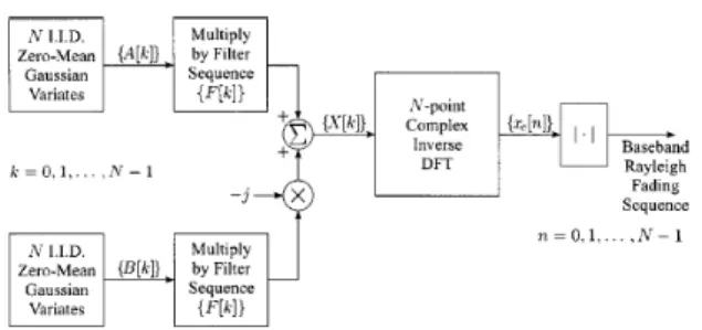
(21) method can simulate Doppler spectrum for double mobility communication environment. But SS method has disadvantage on sampling infinite power spectrum density (PSD). For these reasons, Wang and Cox modified SS method to solve the weakness. They proposed a LS method to approximate the continuous Doppler spectrum as a set of discrete frequencies to generate the received multipath signal as N. 1 Xp rLS (t) = SLS (fn ) exp(−j(2πfn t + φn )) A n=1 SLS (fn ) =. Z N X ¡ n=1. Fn+1. S(f ) df. ¢. δ(f − fn ). (2.3). (2.4). Fn. R Fn+1. f S(f )df fn = RFnFn+1 S(f )df Fn. (2.5). where Fn are the equally spaced sample frequencies, F1 , F2 , . . . , FN +1 with F1 = −(f1 + f2 ) and FN +1 = (f1 + f2 ) and A is a normalize factor to unity the signal power. fn and S(fn ) are the center mass frequencies and corresponding massed, and can be obtain from the integration of the Doppler spectrum in (2.2).. 2.2 2.2.1. Inverse Discrete Fourier Transform Method Smith’s Method. Smith has published an algorithm [21] to generate correlated Rayleigh random variates in fig. 2.1. The method is based on using an inverse discrete Fourier transform (IDFT), to generate two independent vectors of correlated Gaussian samples, which are combined in quadrature to produce a vector of Rayleigh samples. The correlation corresponding to a specified discrete fading spectrum is achieved by multiplication in the frequency domain by appropriate filter coefficients prior to the. 8.

(22) Figure 2.1: Block diagram of the algorithm of Smith to generate correlated Rayleigh variates. IDFT operation. To generate a desired Rayleigh sequence, Smith form a sequence {X[k]}, k = 0, 1, . . . , N − 1, where    X[k] = F [k]A[k] − jF [k]B[k]       F [k] are filter coefficients   A[k] are i.i.d. η(0, σ 2 )      B[k] are i.i.d. η(0, σ 2 )      A[k] and B[k] are independent for all k Taking IDFT on X[k], the Rayleigh sequence is x[n], n = 0, 1, . . . , N − 1, where x[n] =. N −1 1 X 2πkn ) X[k] exp(j N k=0 N. 9. (2.6).

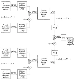
(23) Figure 2.2: Block diagram of the improved algorithm using a single complex IDFT to generate correlated Rayleigh variates.. 2.2.2. Young and Beaulieu’s Method. Figure 2.2 shows Young and Beauliue’s algorithm. Their algorithm is modified from Smith’s method. By a proper change of the filter coefficients F [k], Smith’s method can be modified such that the real part and imaginary part of the single sequence x[n] are uncorrelated for all n. This algorithm is simpler, since the independence between the real and imaginary parts means that the complex output from a single IDFT is directly the complex Gaussian process we require to form the Rayleigh output sequence. The necessity of the second IDFT operation has been eliminated. Thus, the time to execute the procedure is reduced by almost one-half and the memory use for the new routine is one-half to two-thirds that of the original.. 2.3. Sum-of-Sinusoids Approximation Method. The well-known sum-of-sinusoids-based Rayleigh fading channel model is Jake’s model. The purpose of the model is to superimpose the outputs of several sinusoids generators. The ith complex sinusoid is defined by frequency fDi , phase offset θi , and amplitude ci , where 1 ≤ i ≤ Ns and Ns is the total number of sinusoids. Thus, the. 10.

(24) fading process x[n], n = 0, 1, . . . , N − 1, is written x[n] =. Ns X. ci exp(−j(2πfDi n + θi )) .. (2.7). i=1. By central limit theorem, the sum approaches a complex Gaussian random process as the number of generators increase. In practice, the generated sequence closely approximates a Gaussian process if sufficient number of sinusoids is used. But Jake’s model can only used in single mobility environment. Thus, Akki [5,22] and St¨ uber [7] have modified Jake’s model for modelling double mobility communication channels. And my research is followed from their works. From these introductions, we may conclude that sum-of-sinusoids approximation method is better than other methods. This is because LS method involves numerical integrations and IDFT method can not generate longer waveforms without periodicity [7].. 11.

(25) 12. CHAPTER 3 Mobile-to-Mobile Rician Fading Channel Model. 3.1. Introduction. Mobility affects wireless networks significantly. In traditional cellular systems, the base station is stationary and only mobile terminals are in motion. However, in many new wireless system, such as the intelligent transport systems (ITS) and mobile ad hoc networks, a mobile directly connects to another mobile without the help of fixed base stations. Thus, how mobility affects a system where both the transmitter and the receiver move simultaneously becomes an interesting problem. From the propagation perspective, the scattering environment in the mobileto-mobile communication channel is different from that in the base-to-mobile communication channel. In the former case both the transmitted and received signals are affected by the surrounding scatters, whereas in the latter case only the mobile terminal surrounded by many scatters. In a short-distance mobile-to-mobile communication link, a line-of-sight (LOS) or specular component also likely exist between the transmitter and the receiver. In the literature, most channel models for wireless communications were mainly developed for the conventional base-to-mobile cellular radio systems [1–4]. Whether these mobile-to-base channel models are applicable to the mobile-to-mobile commu-.

(26) nication systems is not so clear. In the literature, some but not many channel models were reported. In [5], the theoretical performance of the mobile-to-mobile channel was developed. The authors in [6] introduced the discrete line spectrum method to model the mobile-to-mobile channel. However, the accuracy of this method was assured for only short duration waveforms as discussed in [7]. A simple but accurate sum-of-sinusoids method was proposed to model the mobile-to-mobile Rayleigh fading channel in [7]. The inverse fast fourier transform (IFFT) based mobile-to-mobile channel model was also proposed in [8]. Although most accurate compared to the discrete line spectrum and the sum-of-sinusoids methods, the IFFT-based method requires a complex elliptic integration. However, in [5–8], the LOS effects are all ignored. To evaluate the physical layer performance, a simple channel simulator, such as Jake’s method in conventional cellular systems, is necessary. To our knowledge, such a simulation method for the mobile-to-mobile Rician fading channel is lacking in the literature. Hence, we are motivated to develop a sum-of-sinusoids mobile-tomobile Rician fading simulator. First, we propose the “correlated double ring” model to incorporate the LOS effect and the scattering effect. The double ring scattering model was originally suggested in [7], where the scatterers around the transmitter and the receiver were modelled by two independent rings. Second, we extend the theoretical statistical property of the mobile-to-mobile Rayleigh channel to the Rician fading case. The derived theoretical properties of the mobile-to-mobile Rician fading channel are used to validate the accuracy of the proposed sum-of-sinusoids based mobile-to-mobile Rician fading channel simulator. The rest of this chapter is organized as follows. Section 3.2 describes the system model and the proposed “correlated double ring” scattering model. In Section 3.3 we discuss the sum-of-sinusoids mobile-to-mobile Rician fading simulator. Section 3.4 shows the numerical results. In Section 3.5, we give our concluding remarks. 13.

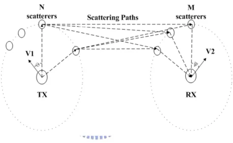
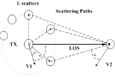
(27) 3.2. Scattering Environment. In this section, we discuss a correlated double-ring scattering model for the mobileto-mobile Rician fading channel. For comparison, we first discuss the independent double-ring scattering model for the mobile-to-mobile Rayleigh fading channel.. 3.2.1. Traditional Double-Ring Scattering Model. Since in a mobile-to-mobile communication channel, the antenna heights of both the transmitter and receiver are below the surrounding objects, it is likely that both the transmitter and the receiver experience rich scattering effect in the propagation paths. In Fig. 3.1, an independent two-ring scattering environment was proposed to characterized the mobile-to-mobile Rayleigh fading channel [7]. Based on this scattering model, a sum-of-sinusoids method was suggested to approximate the mobile-to-mobile Rayleigh fading channel. The scatterers are assumed to be uniformly distributed. Let the transmitter and receiver move at the speeds of V1 and V2 , respectively. For the total N M independent paths, the normalized complex received signal amplitude in the mobile-to-mobile Rayleigh fading channel can be expressed as r Y (t) = where f1 =. V1 λ. N,M 1 X exp[j (2πf1 t cos(αn ) + 2πf2 t cos(βm ) + φnm )] , N M n,m=1. and f2 =. V2 λ. (3.1). are the maximum Doppler frequencies resulted from the. motion of Tx and Rx. In (3.1) 2nπ − π + θn , 4N. (3.2). 2 (2mπ − π + ψm ) , 4M. (3.3). αn = βm =. where the angles of departure in each scattering paths (θn ) and the angle of arrival (ψm ) and φnm in Y (t) are all independent uniformly distributed random variables over 14.

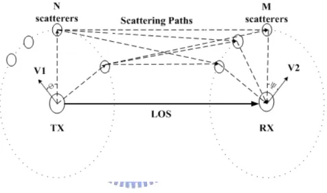
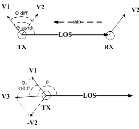
(28) [−π, π). It can be proved that the autocorrelation function of the complex envelope Y (t) is equal to RY Y (τ ) =. J0 (2πf1 τ )J0 (2πf2 τ ) , 2. (3.4). where J0 (·) is the zeroth-order Bessel function of the first kind.. 3.2.2. Correlated Double-Ring Scattering Model. Note that the two rings shown in Fig. 3.1 are mutually independent. In some situations, certain LOS components exist between the transmitter and the receiver. Consequently, the two scattering rings around the transmitter and the receiver are correlated. Figure 3.2 shows the proposed “correlated double ring” scattering model. In addition to the two scattering rings, we add a LOS component between the transmitter and the receiver. It is complex to present the LOS component by a mathematical formula, especially when both the transmitter and the receiver are in motion. Therefore, we use the concept of relative motion to simplify the problem. Figure 3.3 shows the relative velocity (V3 ) of the transmitter to the receiver if the velocity of the receiver is set to be zero. In the figure, θ0 is the angle between V3 and the LOS component. The relative velocity of the transmitter V3 can be derived as follows: q V3 = (V1 · cos(θdif f ) − V2 )2 + (V1 · sin(θdif f ))2 , (3.5) θ0 = θsend + θ31dif f ,. (3.6). where θdif f is the angle between vector V1 and V2 ; θsend is the angle between vector V1 and LOS component and the angle between vectors V3 and V1 is θ31dif f = cos−1 (. V12 + V32 − V22 ) . 2V1 · V3. (3.7). Thus, the LOS component of the mobile-to-base station case can be expressed as LOS =. √. K exp(j (2πf3 t cos(θ0 ) + φ0 )) , 15. (3.8).

(29) where K is the ratio of the specular power to the scattering power, f3 is the Doppler frequency caused by V3 and the initial phase φ0 is uniformly distributed over [−π, π).. 3.3. Sum-of-Sinusoids Rician Fading Simulator. Based on the “correlated double-ring” scattering model shown in Fig. 3.2, we develop a new sum-of-sinusoids Rician fading simulator for the mobile-to-mobile communication.. 3.3.1. Signal Model based on Correlated Double-Ring Scattering. Because Rayleigh fading is a special case of Rician fading without the specular component, the received complex signal of the mobile-to-mobile Rician fading channel is equivalent to the sum of the scattering signal and a LOS component. Therefore, referring to (3.1) and (3.8) the received complex envelope of the mobile-to-mobile Rician fading channel can be written as √ Y (t) + K exp(j (2πf3 t cos(θ0 ) + φ0 )) √ Z(t) = . 1+K. (3.9). Decompose the complex signal Z(t) to the in-phase Zc (t) and the quadrature Zs (t) component. Then it is followed that Z(t) = Zc (t) + j Zs (t) , where Zc (t) =. Yc (t) +. and Zs (t) =. Ys (t) +. √. K cos(2πf3 t cos(θ0 ) + φ0 ) √ , 1+K. √. K sin(2πf3 t cos(θ0 ) + φ0 ) √ . 1+K 16. (3.10). (3.11). (3.12).

(30) 3.3.2. Second-Order Statistics. Now we derive the second order statistical properties of Z(t). The autocorrelation function of Zc (t) can be calculated as RZc Zc (τ ) = E[Zc (t) × Zc (t + τ )] 1 = 1+K. (. h N,M X 1 E cos(2π(f1 cos αn + f2 cos βm )t + φnm ) NM n,m=1. i cos(2π(f1 cos αn + f2 cos βm )(t + τ ) + φnm ). N,M. X. n,m=1. h i + E cos(2πf3 t cos θ0 + φ0 ) cos(2πf3 (t + τ ) cos θ0 + φ0 ) r +. K A+ NM. r. K B NM. ) ,. (3.13). where h N,M i X A=E cos(2π(f1 cos αn + f2 cos βm )t + φnm ) × cos(2πf3 (t + τ ) cos θ0 + φ0 ) = 0 , n,m=1. (3.14) and h. N,M 0. B = E cos(2πf3 t cos θ + φ0 ) ×. X. i cos(2π(f1 cos αn + f2 cos βm )(t + τ ) + φnm ) = 0 .. n,m=1. (3.15) Because φnm , θn , ψm and φ0 are mutually independent random variables, RZc Zc (τ ) can be further simplified as ( N M hX X 1 1 RZc Zc (τ ) = E cos(2πf1 τ cos αn ) cos(2πf2 τ cos βm ) 1 + K NM n=1 m=1 17.

(31) −. N X. sin(2πf1 τ cos αn ). n=1. M X. i sin(2πf2 τ cos βm ). m=1. ) h i + K E cos(2πf3 t cos θ0 ) cos(2πf3 (t + τ ) cos θ0 ) 1 h2 = 1+K π 2 π. Z. +. π 2. 0. Z. π 2. 0. 1 cos(2πf1 τ cos α)dα π. 1 sin(2πf1 τ cos α)dα π. Z. Z. π. cos(2πf2 τ cos β)dβ 0. i. π. sin(2πf2 τ sin β)dβ 0. 1 K cos(2πf3 τ cos θ0 ) . 1+K. (3.16). Consequently, we obtain RZc Zc (τ ) =. J0 (2πf1 τ )J0 (2πf2 τ ) + K cos(2πf3 τ cos(θ0 )) . 1+K. (3.17). Similarly, other time correlation functions of Z(t) can be obtained as follows : RZs Zs (τ ) =. J0 (2πf1 τ )J0 (2πf2 τ ) + K cos(2πf3 τ cos(θ0 )) ; 1+K. (3.18). RZc Zs (τ ) =. K sin(2πf3 τ cos(θ0 )) ; 1+K. (3.19). RZs Zc (τ ) =. −K sin(2πf3 τ cos(θ0 )) ; 1+K. (3.20). J0 (2πf1 τ )J0 (2πf2 τ ) + K exp(j 2πf3 τ cos(θ0 )) . 1+K. (3.21). RZZ (τ ) =. 3.3.3. Signal Model Based on Single-Ring Scattering. For comparison, we briefly show the mobile-to-mobile Rician fading channel model based on the single ring scattering model [5]. In Fig. 3.4, scatterers are distributed around the mobile terminal and there exist a LOS component between the Tx and. 18.

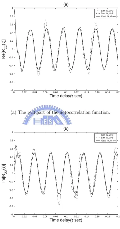
(32) the Rx. Let V1 and V2 be the mobile’s speed and θ0 be the departure angle of the LOS component. In this model, the received signal is the sum of the signals from each scattering paths with a LOS component. That is, r N 1 1 X H(t) = √ { exp(j(2πf1 t cos(αn ) + 2πf2 t cos(βn ) + φn )) N n=1 1+K +. √. K exp(j(2πf3 t cos(θ0 ) + φ0 ))} .. (3.22). It can be shown that the theoretical autocorrelation and cross-correlation functions of the fading signal H(t) of (3.22) are equal to (3.17) - (3.21). 3.4. Numerical Results. In this section, we first validate the proposed sum-of-sinusoids mobile-to-mobile Rician fading simulator. We compare the correlation functions and probability density function (PDF) of the proposed model with the theoretical values. Consider that the maximum Doppler frequency for Tx and Rx is 100Hz and 20Hz, respectively, and θsend = π/5, θdif f = π/3.. 3.4.1. Effects of Numbers of Scatterers. Figure 3.5 shows the simulation results of the autocorrelation of the complex envelope RZZ (τ ) defined in (3.21). As shown in the figure, when the numbers of scatterers N = M = 8, the performance of the the proposed mobile-to-mobile Rician fading channel simulator almost approaches to the ideal case (N, M → ∞).. 19.

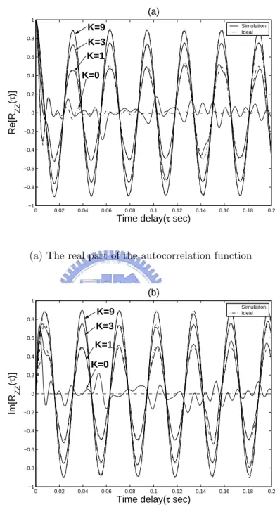
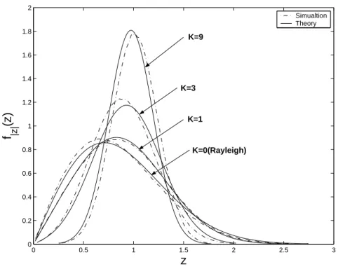
(33) 3.4.2. Effects of Rician Factor. Figure 3.6 shows the correlation properties of the proposed sum-of-sinusoids mobileto-mobile simualtor. The solid line in the figure represents the theoretical value and the dashed line represents the results of the proposed channel model. Clearly, the simulator matches the theoretical values quite well for different Rician factors. Furthermore, for the same delay time τ , the magnitude of the channel correlation (RZZ (τ )) is proportional to the magnitude of the Rician factor (K). Referring to (3.21), one can see that for a large enough delay time τ , J0 (2πf1 τ )J0 (2πf2 τ ) ≈ 0 and J0 (2πf1 τ )J0 (2πf2 τ ) ¿ K exp(2πf3 τ cos(θ0 )). Thus, it is followed that Re{RZZ (τ )} ' Re{ =. K exp(2πf3 τ cos(θ0 ))} 1+K. K cos(2πf3 τ cos(θ0 )) . 1+K. (3.23). Therefore, the maximum amplitude of the autocorrelation function RZZ (τ ) is proportional to. K 1+K. because −1 ≤ cos(2πf3 τ cos(θ0 )) ≤ 1. As K increases, the peaks of. RZZ (τ ) are close to one. Figure 3.7 shows the PDF of the faded signal envelope of the proposed channel model. The PDF of Rician distribution is written as f|z| (z) = 2(1 + K)z · exp[−K − (1 + K)z 2 ] ×I0 [2z. p K(1 + K)] ,. (3.24). where K is the Rician factor and I0 (·) is the zeroth-order modified Bessel function of the first kind. The simulation results show that the PDFs of our proposed channel model are very close to the theoretical values when N = M = 8.. 20.

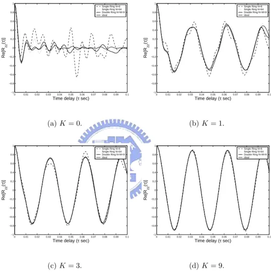
(34) 3.4.3. Comparison of Correlated Double-Ring and Single-Ring Models. In this part, we compare our proposed mobile-to-mobile Rician channel model based on the correlated double-ring scattering model with the one based on the single-ring scattering model [17] for different Rician factors and different numbers of scatterers. The main purpose of the comparison is to demonstrate that it is more suitable to apply the double-ring scattering model to characterize the mobile-to-mobile communication channel. From previous discussions, we know that these two method lead to the same theoretical value. Thus, we have to compare their simulation results to determine which one is closer to the ideal values. Figure 3.8 shows the correlation of the doublering model with 8 scatterers, the single-ring model with 8 scatterers, single-ring model with 64 scatterers and the theoretical correlation functions. Obviously, double-ring model yields better performance than single ring model even if we use 64 scatterers in single-ring model. The difference of the two scattering models is significant when K is medium-sized or small. Figure 3.9 shows the deviation between the simulated and theoretical correlations for the two different models with various values of K. For both models, the deviation decreases with the increase of K, but the results for the double-ring scattering model still have better performance and less computational loads.. 3.5. Conclusions. In this chapter, we have developed a sum-of-sinusoids-based mobile-to-mobile Rician fading simulator. We propose the correlated double ring scattering model to characterize the mobile-to-mobile communication environment with LOS components. Furthermore, we also derive the theoretical correlation functions of mobile-to-mobile. 21.

(35) Rician channel and verify its accuracy by simulations. Last, we prove that the proposed sum-of-sinusoids approximation based on the correlated double-ring model can approach the theoretical value more closely than the single-ring model at a slightly higher cost of computation loads.. 22.

(36) Figure 3.1: The independent two-ring scattering model for the mobile-to-mobile Rayleigh fading channel.. 23.

(37) Figure 3.2: Scattering environment in a mobile-to-mobile system with a LOS component.. 24.

(38) Figure 3.3: Relative velocity V3 from the TX with velocity V1 to the RX with velocity V2 .. 25.

(39) Figure 3.4: Single-ring scattering environment for a mobile-to-mobile Rician fading channel.. 26.

(40) (a) 1 Sim N,M=3 Sim N,M=8 Ideal N,M→∞. 0.8. 0.6. Re[RZZ(τ)]. 0.4. 0.2. 0. −0.2. −0.4. −0.6. −0.8. −1. 0. 0.02. 0.04. 0.06. 0.08. 0.1. 0.12. 0.14. 0.16. 0.18. 0.2. Time delay(τ sec). (a) The real part of the autocorrelation function.. (b) 1 Sim N,M=3 Sim N,M=8 Ideal N,M→∞. 0.8. 0.6. Im[RZZ(τ)]. 0.4. 0.2. 0. −0.2. −0.4. −0.6. −0.8. −1. 0. 0.02. 0.04. 0.06. 0.08. 0.1. 0.12. 0.14. 0.16. 0.18. 0.2. Time delay(τ sec). (b) The image part of the autocorrelation function.. Figure 3.5: The autocorrelation function of the complex envelope Z(t), where K = 1.. 27.

(41) (a) 1. K=9 0.8. K=3 K=1. 0.6. K=0. 0.4. Re[RZZ(τ)]. Simulaiton Ideal. 0.2. 0. −0.2. −0.4. −0.6. −0.8. −1. 0. 0.02. 0.04. 0.06. 0.08. 0.1. 0.12. 0.14. 0.16. 0.18. 0.2. Time delay(τ sec). (a) The real part of the autocorrelation function. (b) 1 Simulaiton Ideal. K=9 0.8. K=3 0.6. K=1 0.4. Im[RZZ(τ)]. K=0 0.2. 0. −0.2. −0.4. −0.6. −0.8. −1. 0. 0.02. 0.04. 0.06. 0.08. 0.1. 0.12. 0.14. 0.16. 0.18. 0.2. Time delay(τ sec). (b) The image part of the autocorrelation function.. Figure 3.6: The autocorrelation function of the complex envelope Z(t), where N = M = 8 for K = 0, 1, 3, and 9. 28.

(42) 2 Simualtion Theory 1.8. K=9. 1.6. 1.4. K=3. f|z|(z). 1.2. K=1 1. K=0(Rayleigh). 0.8. 0.6. 0.4. 0.2. 0. 0. 0.5. 1. 1.5. 2. 2.5. 3. z. Figure 3.7: The PDF of the fading envelope Z(t) when N = M = 8.. 29.

(43) 1. 1 Single Ring N=8 Single Ring N=64 Double Ring N=M=8 ideal. 0.6. 0.6. 0.4. 0.4. zz. 0.2. 0. −0.2. 0.2. 0. −0.2. −0.4. −0.4. −0.6. −0.6. −0.8. −0.8. −1. 0. 0.01. 0.02. 0.03. 0.04. 0.05. 0.06. 0.07. 0.08. 0.09. Single Ring N=8 Single Ring N=64 Double Ring N=M=8 ideal. 0.8. Re[R (τ)]. Re[Rzz(τ)]. 0.8. −1. 0.1. 0. 0.01. 0.02. 0.03. Time delay (τ sec). (a) K = 0. 1. 0.06. 0.07. 0.08. 0.09. 0.1. 1 Single Ring N=8 Single Ring N=64 Double Ring N=M=8 ideal. Single Ring N=8 Single Ring N=64 Double Ring N=M=8 ideal. 0.8. 0.6. 0.6. 0.4. 0.4. Re[R (τ)]. 0.2. zz. Re[Rzz(τ)]. 0.05. (b) K = 1.. 0.8. 0. −0.2. 0.2. 0. −0.2. −0.4. −0.4. −0.6. −0.6. −0.8. −1. 0.04. Time delay (τ sec). −0.8. 0. 0.01. 0.02. 0.03. 0.04. 0.05. 0.06. 0.07. 0.08. 0.09. −1. 0.1. Time delay (τ sec). 0. 0.01. 0.02. 0.03. 0.04. 0.05. 0.06. 0.07. 0.08. 0.09. 0.1. Time delay (τ sec). (c) K = 3.. (d) K = 9.. Figure 3.8: The real part of the fading envelope of double-ring and single-ring scattering models.. 30.

(44) 0.2. Single Ring Model Double Ring Model. 0.18. 0.16. Deviation. 0.14. 0.12. 0.1. 0.08. 0.06. 0.04. 0.02. 0. 1. 2. 3. 4. 5. 6. 7. 8. 9. 10. K. Figure 3.9: The difference of the real part of the fading envelope Z(t) based on the double-ring scattering model from that based on the single-ring scattering model when K varies from 0.1 to 20.. 31.

(45) 32. CHAPTER 4 Average Fade Duration of Mobile-to-Mobile Rician Fading Channels Statistical properties of mobile-to-mobile Rician fading channel has been developed in the previous chapter, but these properties may not sufficient to describe the channel characteristics. Thus, we are motivated to derive higher-order characteristics of the fading channel. In this chapter, we derive the level-crossing rate (LCR) and average fade duration (AFD) of the fading envelope of a mobile-to-mobile Rician fading channel. Through the LCR and AFD analysis, we may investigate the impact of the line-of-sight component and terminal mobility on the channel fading behavior.. 4.1. Introduction. In Chapter 3, we have developed a sum-of-sinusoids based mobile-to-mobile Rician simulator to simulate the mobile-to-mobile Rician fading channel and we have find out its second-order characteristics. But these properties may not provide enough information about the channel fading behavior. Thus, we are motivated to concentrate on the higher-order channel characteristics, such as the level-crossing rate and average fading duration of fading envelope. These high order characteristics may help us to determine the temporal behavior of the channel fading. Moreover, it may assist system developers to generally understand the channel fading in various channel sta-.

(46) tus, and will also aid them to make their decision on choosing sufficient radio resource allocation mechanism. The rest of this chapter is organized as follows. Section 4.2 derives the LCR and AFD of the mobile-to-mobile Rician fading channel. Section 4.3 compares the simulated LCR and AFD to the theoretical values. Finally, we give our concluding remarks in Section 4.4.. 4.2 4.2.1. Higher-Order Statistics Level-Crossing Rate. Denote α(t) the fading envelope |Z(t)| , α(t) ˙ the derivative of the fading envelope ˙ |Z(t)|, p (α) the probability density function (PDF) of the fading envelope, and p (α) ˙ the PDF of the slope of the fading envelope. Then the level crossing-rate (LR ) of the fading envelope |Z(t)| with respect to of a specified level R can be calculated by [23] Z ∞ α˙ pα,α˙ (R, α)d ˙ α˙ (4.1) LR = 0. where pα,α˙ (α, α) ˙ is the joint distribution function of α and α. ˙ Now, the key issue is to find the joint distribution pα,α˙ (α, α). ˙ From [22] and [24], we know that the joint distribution of fading envelope and envelope slope of a Rician fading signal can be expressed as [25] r 1 α˙ 2 α (α2 + s2 ) αs pα,α˙ (α, α) ˙ = exp{− } exp{− }I0 ( ) 2πb2 2b2 b0 2b0 b0. (4.2). where s2 = E[gI (t)]2 + E[gQ (t)]2 ; Ωp = E[α2 ] = s2 + 2b0 ; 33. (4.3).

(47) s2 =. KΩp Ωp ; 2b0 = ; K +1 K +1. Ωp is the square mean of the fading envelope; s2 is the power of the specular component and 2b0 is the scattered power. From (4.2), it is implied that pα (α) and pα˙ (α) ˙ are mutually independent. Thus, we have r 1 α˙ 2 pα˙ (α) ˙ = exp{− } , 2πb2 2b2. (4.4). and pα (R) =. α (α2 + s2 ) αs exp{− }I0 ( ) . b0 2b0 b0. (4.5). The LR can be simplified as Z. ∞. LR = pα (R). αp ˙ α˙ (α)d ˙ α˙. (4.6). 0. r = pα (R). b2 2π. where b2 = −d2 RZZ (τ )/dτ 2 |τ =0 [22]. Recall that the auto-correlation function RZZ (τ ) of the faded signal Z(t) is derived in (3.21). After derivative, b2 can be express as b2 =. 1 (2π)2 (f12 2. + f22 ) + K(2π)2 f32 cos2 θ0 1+K. (4.7). where Doppler frequency f1 = V1 /λ, f2 = V2 /λ, and λ is the carrier wavelength. Substituting (4.3) and (4.7) into (4.6), we obtain r R2 b2 2(K + 1) R p LR = · p exp(−K − (K + 1) ) 2π Ωp Ωp Ωp. (4.8). R p I0 (2 p K(K + 1)) Ωp where K is the Rician factor and I0 (·) is the modified zero-order bessel function of the first kind.. 34.

(48) 4.2.2. Average Fade Duration. According to the definition in [23], the average-fading duration (¯ τR ) for a specified level R is τ¯R =. p(α ≤ R) . LR. (4.9). Since the envelope of the signal is Rician distributed, τ¯R can be expressed as p √ 1 − Q( 2K, 2(K + 1)R2 ) , (4.10) τ¯R = LR where the Marcum Q function is defined as Z ∞ (x2 + a2 ) Q(a, b) = x exp(− )I0 (ax)dx . 2 b. 4.3. (4.11). Numerical Results. Here we show the LCR and AFD of a mobile-to-mobile Rician channel fading envelope based on the sum-of-sinusoids method and the theoretical value, respectively. The simulation model of the mobile-to-mobile Rician fading channel have been develop in chapter 3. Through the simulations, we could observe what is the impact of the terminal mobility and LOS component on the channel fading. Figure 4.1 shows the LCR of a mobile-to-mobile Rician channel fading envelope based on the sum-of-sinusoids method and those based on theoretical analysis. It is shown that the LCR decreases with the increase of the Rician factor. This phenomenon can be explained by the fact that the channel fading has greater correlation with larger amount of LOS component. Once the correlation arises, the changing of the channel fading decreases. Figure 4.2 shows the theoretical values of the normalized AFD with different Rician factors. As shown in the figure, the larger the Rician factor, the larger the 35.

(49) AFD. This property is caused by higher correlation of fading envelope for a larger Rician factor. Thus, if the signal envelope is faded below a specified level, it has smaller probability to exceed the level.. 4.4. Conclusions. In this chapter, we have find out the theoretical LCR and AFD of mobile-to-mobile Rician fading channel. Another contribution is that we derived the probability distribution of the slope of the fading envelope, which is obtained from the ACF of the mobile-to-mobile Rician fading channel in chapter 3. In the last part, we validate the LCR and AFD from simulations. We also observer the influence of the LOS component and terminal mobility on the channel fading.. 36.

(50) Figure 4.1: Normalized envelope level crossing rate for mobile-to-mobile Rician fading. Solid line denotes the theoretical results and the dashed line denotes the simulation results, where ρ = √R . Ωp. 37.

(51) Figure 4.2: Normalized average fade duration for a mobile-to-mobile Rician fading channel for K = 10, 7, 3, and 1.. 38.

(52) 39. CHAPTER 5 Capacity Analysis of MIMO Mobile-to-Mobile Rician Fading Channels. 5.1. Introduction. Digital communication using the multiple-input multiple-output (MIMO) antenna technique has emerged as one of most significant breakthroughs in communications recently. The fourth generation (4G) cellular system [9] and the next generation high speed IEEE 802.11n [10] wireless local area network (WLAN) all adopt the MIMO technique to deliver capacity and diversity gains. In the mean-while, another communication paradigm - ad hoc networks - has become important alternative for the next generation wireless systems. In contrast to conventional cellular systems with master-slave relation between base station and mobile users, nodes in ad hoc networks adopts peer-to-peer communication. Specifically, this type of communication is supported by direct connection or multiple hop relays without fixed wireless infrastructure. The concepts of ad hoc networks have been enabled in many standards such as Bluetooth and IEEE 802.11 WLAN. Ad hoc networking is considered as the key enabling technique of many future wireless systems, such wireless mesh networks [11] and cognitive radio [12]. Unlike conventional mobile-to-fixed base station systems that have been benefited by the MIMO technique, how and to what extend the ad hoc networks can.

(53) benefit from the MIMO technique is still an open research area. One fundamental issue is how to accurately model the impact of spatial/temporal correlation on MIMO capacity form a view point of the mobile-to-mobile communication. Scattering model and the line-of-sight (LOS) component are two important factors needed to be considered. First, in a mobile-to-mobile environment, the antenna heights of both the transmitter and the receiver are lower than the surrounding objects. Thus, the signal in a mobile-to-mobile environment will experience a richer scattering effect than in a mobile-to-base environment [7, 13, 14]. Second, a LOS component may more likely exist in a short distance mobile-to-mobile application than in a long distance mobileto-base environment. In [15], the distribution of the Rician K factor was modelled as lognormal, with the median as a function of distance: K ∝ (distance)−0.5 . Implicitly, the K factor increases as the distance decreases. Thus, the Rician fading effect can not be neglected in a short-distance mobile-to-mobile communication environment. The objective of this chapter are two folds. First, we aim to develop a simple sum-of-sinusoids MIMO channel simulation method that can characterize the spatial/temporal correlation and Rician fading effect. The sum-of-sinusoids channel simulation method, or called the Jake’s model, has been widely used to evaluate the performance of conventional single-input single-output (SISO) mobile systems [2, 16, 17]. The Jake’s model can capture the time behavior of a mobile-to-base channel. Recently, in [13], a mobile-to-mobile MIMO channel simulator was developed to incorporate the spatial correlation in a Rayleigh fading environment. We will further incorporate Rician fading effect in the mobile-ro-mobile MIMO channel simulator based on a correlated double-ring scattering model. (described in Section 5.2) The second objective of this chapter is to investigate the capacity of the mobileto-mobile MIMO Rician fading channel. To this end, we will derive the upper bound of the ergodic capacity of the mobile-to-mobile MIMO Rician channel. The MIMO capacity bound can be used to validate the accuracy of the proposed sum-of-sinusoids 40.

(54) simulation method and investigate the impact of spatial correlation. The rest of this chapter is organized as follows. Section 5.2 describes the scattering model for the mobile-to-mobile communication system. In Section 5.3, we introduce the sum-of-sinusoids MIMO Rician fading simulator. In Section 5.4, we evaluate the ergodic capacity and capacity fade duration of the MIMO Rician fading channel based on the proposed simulation method. In Section 5.5, we show numerical results to elaborate the impacts of Doppler frequency, the Rician K factor, spatial correlation, and temporal correlation on the MIMO mobile-to-mobile systems. We give our concluding remarks in Section 5.6.. 5.2. Scattering Model. In this section, we introduce the correlated correlated double-ring scattering model [14]. This model can be used to capture the scattering effect and the LOS effect in a mobile-to-mobile environment as shown in Fig. 5.1. In the figure, the transmitter and the receiver moving at a speed of V1 and V2 m/sec, are surrounded by I and N scatterers, respectively. The angles of departure (AOD) between vector V1 and scattering paths are denoted by θti (i = 1, 2, · · · , I.), and θrn (n = 1, 2, · · · , N.) are the angles of arrival between vector V2 and scattering paths. Assume that θti and θrn are independent and uniformly distributed over [−π, π). Note that there exist LOS components between the transmitter TX and the receiver RX, where both TX and RX are equipped with multiple antennas. Consider that the multiple antennas are separated by the distance d. In the case that the transmission distance from the scatterers to the receive antenna is much longer than d, then the angle of arrival (AOA) from the n-th scatterer to each receive antenna will be about the same, i.e. θrn . Thus, as shown in Fig. 5.2, for the case with two receive antennas, the transmission distance from the n-th scatterer to the 41.

(55) Figure 5.1: Correlated double-ring scattering model with LOS components.. second receive antenna is d · cos θrn longer than that to the first receive antenna.. 5.3. Sum-of-Sinusoids MIMO Rician Fading Simulator. 5.3.1. Line-of-sight Component Model. To begin with, we discuss the approach to model the LOS component between each pair of moving transmit and receive antennas. For simplicity, we first consider the single antenna case. Referring to Fig. 5.3(a), let the transmitter TX moves at a speed of V1 toward the direction of the angle θβ relative to the receiver RX’s velocity V20 s direction, where θα is the angle between V1 and the transmission direction of the LOS component. Using the concept of the relative motion [26], let the RX’s velocity be zero and denote V3 the relative velocity from TX to RX, as shown in Fig. 5.3(b). In. 42.

(56) Figure 5.2: Received signals at multiple antennas with an AOA θrn and separation distance d under the assumption that the transmission distance is much longer than d. the figure, θ0 is the angle between V3 and LOS component. The relative velocity V3 can be derived as follows: V3 =. q (V1 · cos(θβ ) − V2 )2 + (V1 · sin(θβ ))2 , θ0 = θα + θγ ,. (5.1) (5.2). and θγ = cos−1 (. V12 + V32 − V22 ) , 2V1 · V3. (5.3). where θγ is the angle between velocity vectors V3 and V1 . Thus the LOS component can be express as LOS =. √. K exp(j (2πfc t − 2πf3 t cos(θ0 )) ,. (5.4). where the Rician K factor is defined as the ratio of the specular power to the scattering power [17]. Now we consider the scenario with multiple antennas. From Fig. 5.3(c), the LOS components for H11 and H21 from the first antenna of TX to both antennas of 43.

(57) RX can be respectively expressed as p. 0 K11 exp(j (2πfc t − 2πf3 t cos(θ11 )). (5.5). 0 K21 exp(j (2πfc t − 2πf3 t cos(θ21 )) ,. (5.6). and p. 0 0 where K11 and K21 are the Rician factors; θ11 and θ21 are the angles from the LOS. components LOS11 and LOS21 to the velocity vector V3 . Assume that the transmission distance between the two mobiles is much longer than the antenna separation d. Then, 0 0 0 0 0 0 the angles θ11 and θ21 are about the same. Likewise, θ21 = θ22 = θ11 = θ12 . To ease. notation for all m and l, let 0 ρ = 2πfc t − 2πf3 t cos(θml ) .. 5.3.2. (5.7). Sum-of-Sinusoids Simulation Method. Based on the correlated double-ring scattering model and the LOS component model. We suggest the sum-of-sinusoids simulation method, for a mobile-to-mobile MIMO channel model with LOS components. Consider narrow band signals in a flat Rician fading channel. The MIMO channel is expressed as an M × L matrix, where M and L are the numbers of antennas at the receiver and transmitter, respectively. Hml , the element of the m-th row and l-th column, is the complex channel gain between the l-th transmit antenna and m-th receive antenna. With this notation, we have I,N X p 1 1 {√ Ain exp(jφin ) + K11 exp(jρ)} , 1 + K11 IN i=1,n=1. (5.8). φin = 2πfc (t − τin ) − 2πf2 (t − τin ) cos(θrn ) − 2πf1 (t − τin ) cos(θti ) ,. (5.9). H11 = √ where. 44.

(58) Figure 5.3: LOS component model for moving transmitter TX and receiver RX of which vectors are V1 and V2 with a relative angle of θβ , respectively.. 45.

(59) fc , f1 =. V1 λ. and f2 =. V2 λ. are the carrier frequency, the maximum Doppler frequencies. resulted from the motion of TX and RX, I and N are the numbers of the scatterers around TX and RX, respectively. τin is the transmission delay of the in-th scattering path. For H21 , we further consider the additional transmission delay due to the antenna separation d. Accordingly, it is followed that H21 = √. I,N X 1 1 {√ Ain exp(jφin + 1 + K21 IN i=1,n=1. jβd(2 − 1) cos(θrn )) +. p. K21 exp(jρ)} ,. (5.10). where β = 2π/λ is the wave number. Thus, the general form of the channel Hml can be computed by Hml = √. I,N X 1 1 {√ Ain exp(jφin + 1 + Kml IN i=1,n=1. jβd(m − 1) cos(θrn ) + jβd(l − 1) cos(θti )) p + Kml exp(jρ)} ,. (5.11). for every m = 1, 2, ..., M , and l = 1, 2, ..., L.. 5.4. Capacity Evaluation. Consider an M × L MIMO channel matrix, assume that the knowledge of a frequency flat faded signal can be known perfectly at the receiver. Let, n be an M × 1 zero mean complex AWGN noise vector, of which the covariance matrix is equal to σ 2·IM . The M × 1 received signal vector y can be expressed as [27] y = Hx + n , 46. (5.12).

(60) where x is an L × 1 transmitted signal vector. The time-varying capacity of a MIMO channel can be written as [28–30]    C = log2 det[ IM + ( SNR ) · HH† ] if M < L  L  (5.13)     C = log det[ I + ( SNR ) · H† H ] if M ≥ L M 2 L where † denotes transpose conjugate and IM denotes an M × M identity matrix. In this part, we derive the channel correlation and find its channel capacity. The channel correlation between H11 and H21 is [13] ∗ ∆11,21 = E[H11 H21 ] ,. (5.14). where ∗ is the complex conjugate. Assume that the number of scatterers around transmitter and receiver equals N ; Ain is zero mean unit variance normal distributed random variable; θti and θrn are uniformly distributed random variables. All of the above random variables are mutually independent. Then, we have √ √ {J0 (βd) + K11 K21 } √ ∆11,21 = √ . 1 + K11 1 + K21. (5.15). The general form of the channel correlation between Hml and Hpq should be expressed as ∆ml,pq. p √ {J0 (βd(m − p))J0 (βd(l − q)) + Kml Kpq } p = , √ 1 + Kml 1 + Kpq. (5.16). where J0 (·) is the zeroth-order Bessel function of the first kind. From (5.13), the average capacity of the MIMO channel can be expressed as CE = E[ log2 det( IM + (. SNR ) · HH† )] . L. (5.17). By using Jensen’s inequality, we conclude that the average capacity is bounded by CE ≤ log2 det( IM + ( 47. SNR ) · E[HH† ] )] . L. (5.18).

(61) Time and Ensamble Average (K=3) 1 Time Average Ensamble Average. 0.9. 0.8. Probability. 0.7. 0.6. 0.5. 0.4. 0.3. 0.2. 0.1. 0. 8. 10. 12. 14. 16. 18. 20. Capacity. Figure 5.4: The time and the ensamble average capacity outage probability of a 3 × 3 MIMO channel when K = 3, SNR = 20 dB, and d = λ/2. R denotes the correlation channel matrix E[HH† ], where √ p L L X X J0 (βd(i − j)) + Kiv Kjv ∗ p Rij = E[Hiv Hjv ] = . √ 1 + K 1 + K iv jv v=1 v=1. (5.19). Thus, we can derive the entire correlation channel matrix R and channel capacity from (5.19). Substituting R into (5.18), we can find out the mobile-to-mobile MIMO channel capacity upper bound.. 5.5. Numerical Results. In our simulation, we randomly generate the mobile-to-mobile MIMO channel matrix H and calculate the channel capacity of H according to (5.17). The purposes of simulations are the following. First, we want to prove the ergodicity of our MIMO channel capacity model by examining time and ensamble averages. Second, we eval48.

(62) Figure 5.5: MIMO Rician Capacity with different Doppler frequencies where SNR = 20 dB, d = λ/2 ,K = 3.. uate the capacity of MIMO Rician fading channel with different Doppler frequencies. Then, we vary the numbers of scatterers to inspect the scattering effect to the MIMO channel capacity. Finally, we vary the antenna separations and the Rician factors to investigate the relationship between spatial channel correlation and channel capacity.. 5.5.1. Ergodicity. Figure 5.4 shows the capacity outage probability of a time average and an ensamble average for a mobile-to-mobile Rician MIMO channel. From the figure, one can see that these two averages were match quite well. This property implies that our channel model is ergodic.. 49.

(63) Figure 5.6: Effect of antenna separation on the ergodic capacity of a 3 × 3 MIMO channel for SNR = 20 dB and various values of K factors.. 5.5.2. Impacts of Doppler Frequencies. Figure 5.5 shows the impact of various Doppler frequencies on the capacity of a 3 × 3 MIMO channel with SNR = 20 dB, d = λ2 , and K = 3. From the simulations, we observe that the LCR of the capacity is proportional to the Doppler frequency, but the mean and the variance of the capacity remain about the same. This result tells us that in a mobile-to-mobile MIMO communication environment the speed of the mobilities will not affect the average channel capacity but will influence the accuracy of channel estimation. This property have not been shown in [13], because that φin is assumed to be uniformly distributed random over [−π, π) in (5.9). In our model, we relax this assumption and generate the time function φin (t). Thus, the temporal behaviors of the channel capacity based on the sum-of-sinusoids method can be observed.. 50.

(64) Figure 5.7: The ergodic capacity of MIMO channles against the number of antennas when SNR = 20 dB, and d = λ/2.. 5.5.3. Effect of Spatial Correlation. Figure 5.6 shows the capacity of a 3 × 3 mobile-to-mobile MIMO channel for different Rician K factor and antenna separation d. The capacity obtained by simulation are lower than its upper bound. In general, we find that the MIMO capacity grows with the increase of the antenna separations when d ≥. λ , 10. and it reach the maximum when. d ' λ2 . We also find that the capacity is vibrated when d become very larger. This phenomenon is resulted from of the Bessel function in (5.16). Recall that the tail of the Bessel function is cosine vibration and its amplitude is exponentially decreased. For the fixed antenna separation, the other source of channel correlation is from the Rician factor. Based on (5.16), if the channel correlation arises, the capacity reduced at the same time. Therefore, if the capacity with K = 3 shows in the figure is lower than that with K = 0 and K = 1.. 51.

(65) Figure 5.8: Capacity per antenna against the number of antennas when SNR = 20 dB, d = λ/2.. 5.5.4. Impact of Numbers of Antennas. Figures 5.7 and 5.8 show the effect of various numbers of antennas on the channel capacity and the capacity per antenna of a MIMO channel, respectively, when d =. λ 2. and K = 0, 3, 5. It is well known that MIMO channel capacity is in proportional to the number of antennas [28–30]. From the figure, however, we observe that the capacity will no longer linearly increase as the number of antennas increases. The total channel capacity increase slowly when the number of antennas exceeds about 20. Thus it is not a wise idea to increase the number of antennas without limitation.. 5.5.5. Impact of Numbers of Scatterers. Figure 5.9 shows the effect of various numbers of scatterers on the total channel capacity of a MIMO system, when d =. λ 2. and K = 0. Here we set K to zero to neglect. 52.

(66) 90 N=M=40 N=M=20 N=M=8. 80. 70. CE bps/Hz. 60. 50. 40. 30. 20. 10. 0. 0. 2. 4. 6. 8. 10. 12. 14. 16. 18. 20. Number of Antennas in mobiles. Figure 5.9: The ergodic capacity of MIMO channels against the number of antennas when SNR = 20 dB, d = λ/2 and K = 0.. the effect of LOS component on the channel capacity and observe the effect of the number of scatterers. From the figure, we found that the total capacity increases with the increase of the numbers of scatterers. This result is quite different from the Fig. 5.7, this is mainly because that the total channel capacity is related to the richness of the scatterers. Thus, if we want to obtain higher channel capacity by increasing the number of antennas, we must have to consider the scattering environment.. 5.6. Conclusions. In this chapter, we have developed a sum-of-sinusoids simulation method for the MIMO in a mobile-to-mobile fading channel. Based on the “correlated double ring” scattering model [14], we incorporate the effect of Doppler effects, antenna separation and LOS components for the MIMO system in a mobile-to-mobile environment. We. 53.

(67) have also derived the capacity upper bound of the mobile-to-mobile MIMO Rician channel. The channel capacity has been validated through simulations. We find that for MIMO systems with constant number of scatterers, increasing number of antennas cannot linearly increase the capacity. The capacity per antenna is decreased more as Rician factor increases. We also find that the total channel capacity is related to the richness of the scattering environment.. 54.

(68) 55. CHAPTER 6 Higher Order Statistics of Mobile-to-Mobile MIMO Rician Channels. 6.1. Introduction. In this chapter, we will study the characteristics of the capacity for a mobile-to-mobile MIMO Rician fading channel. we evaluate the level-crossing rate (LCR) and average fading duration (AFD) of the MIMO mobile-to-mobile Rician channel. The LCR and AFD of MIMO capacity was investigated in [18, 19], but not in a mobile-to-mobile and not in a Rician fading channel, either. We will relate the LCR and capacity fade of MIMO mobile-to-mobile systems with Rician K factor. The rest of this chapter is organized as follows. Section 5.2 derived the approximate distribution, LCR and AFD of the MIMO channel capacity. Section 5.3 shows the numerical results. Finally, we give our concluding remarks in Section 5.4.. 6.2. Level Crossing Rate and Average Fade Duration. Figure 6.1 shows the channel capacity under different doppler frequencies in a time interval. We can easily find that the temporal behavior of the channel capacity is.