An Implementation for Subcube Based Query Processing

全文

(1)Int. Computer Symposium, Dec. 15-17, 2004, Taipei, Taiwan.. An Implementation for Subcube Based Query Processing Huei-Huang Chen Tatung University hhchen@ttu.edu.tw. Kuo-Wei Ho Tatung University d8706001@ms2.ttu.edu.tw. Cheng-Ling Shiou Tatung University g9106008@ttu.edu.tw. to answer a query by scanning the table. Appropriate as these subcubes may be, they may not be the best choice. The best choice is the "nearest parent" [8] based on the subcube computational dependency. To avoid incurring the extra cost of selecting the best subcube from several appropriate ones, a tree structure constructed from the data cube lattice is maintained to keep the computational dependency of subcubes. The tree called Subcube Dependency Tree (SDT) is designed to prune the search space down to a subset of potentially appropriate subcubes. Each node of the tree is a subcube fragment. In this paper, algorithms for SDT management (insertion, deletion and adjustment of SDT nodes) and searching appropriate subcubes for OLAP queries are proposed.. Abstract-Data cube materialization is commonly used in reducing OLAP response time. However, materializing a whole data cube requires large disk space as the focus on the interested subjects results in only a small portion of data cubes being frequently accessed. The subcube, a finer partition of a data cube, is proposed. The subcubes are formed from multi-dimensional queries, and the number of subcubes grows when various queries issued by users with different dimension levels and value ranges. The management framework of these subcubes is important. The technique for searching the subcubes directly affects the query performance, and therefore binary trees and linked lists are used to manage the subcubes. For saving the query processing time, an algorithm for searching appropriate subcubes is proposed.. 2. Related Works Data warehouses come to fill a gap in the field of querying large, distributed and frequently updated systems. Data are extracted from several data sources, cleansed, customized and inserted into the data warehouse. OLAP is one of the analysis tools supported by data warehouses. [3] generalizes OLAP query operators as aggregation, subtotaling, cross tabulation, and grouping. To select views to be materialized for reducing OLAP computing cost, [4] proposed a lattice framework frequently used by view selection algorithms, and it captures the computational dependencies among the data cubes. The static view selection method requires large disk space to store a whole data cube. Research by Yu. Keywords: data cube, materialization, subcube, query processing.. 1. Introduction In most cases, OLAP execution is expensive because answering a query with aggregation entails processing numerous details from the fact tables in the data warehouse. Materialized views have long been proposed to speed up query processing. The most common practice is applying view selection algorithms on search lattice in advance as an undividable unit and then picking up some nodes for materialization. Research by Huei-Huang Chen and Kuo-Wei Ho [1] suggest that most OLAP queries merely focus on some nodes and even some regions within the nodes. That means only a small portion of the materialized nodes is accessed. A subcube-based implementation framework is proposed to further partition a node in a lattice into subcubes for materialization. Thus, storage space is saved. In OLAP query processing, the most important issue is to find the appropriate subcubes for a query efficiently in order to reduce the query processing cost. A subcube's identifier (a combination of subcube cell and subcube class) is adequate for a query cell to check whether it can be answered from the subcube or not. A Subcube Table Method (STM) is introduced to store subcube's information in a RDB table. Appropriate subcubes are then searched. Feng and Shan Wang [2] proposes a method to build a compressed data cube by a clustering technique and use this compressed data cube to provide approximate answers to queries directly.. [1] states that most OLAP queries merely focus on some nodes and even some regions within nodes. A subcube-based implementation framework is proposed to further partition a node in a lattice into subcubes for materialization. The subcubing methods have the following two advantages: First, the unit for materialization can be reduced from a node in a lattice to a finer partition. Second, the drilldown operation in all dimensions will not result in a partition that is too fine to take possible locality effect into consideration. Smith et al. [7] proposes a method for adaptively representing multidimensional. 160.

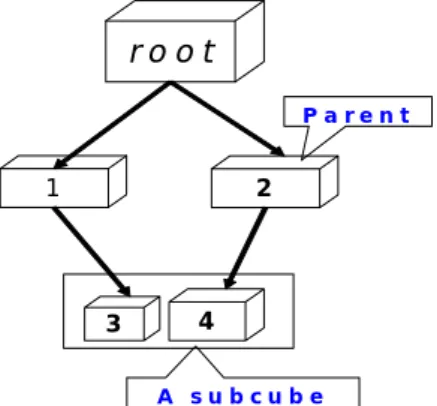
(2) Int. Computer Symposium, Dec. 15-17, 2004, Taipei, Taiwan.. data cubes using wavelet view elements in order to more efficiently support data analysis and querying involving aggregations. The proposed method decomposes the data cubes into an indexed hierarchy of wavelet view elements. The view elements differ from traditional data cube cells in that they correspond to partial and residual aggregations of the data cube. The view elements provide highly granular building blocks for synthesizing the aggregated and range-aggregated views of the data cubes.. another. Computing can span across more than two levels of the SDT as the computational dependency of nodes is kept in the branches of the tree.. 3.2 Construction of the SDT One main job of a subcube based query processor is to find the appropriate subcubes for queries and then use the found subcubes to compute the results. At the same time, the corresponding subcube is checked if it is worth materializing. When the subcube deserves materialization, it is computed by the query processor and stored in the pool for future use, as shown in Figure 2. These newly formed fragments for a subcube are all inserted into the SDT as child nodes of their parents from whom they are computed one by one.. 3. Subcube Dependency Tree The disadvantages of employing Subcube Table Method (STM) are its inefficiency in checking all the subcubes in the table and the overhead of picking up the nearest subcubes. To address these problems, a data structure called Subcube Dependency Tree (SDT) is proposed.. Materialization Admission. ? Subcube. 3.1 Nodes of the SDT The SDT is a tree structure formed of nodes, the subcube fragments. A subcube fragment computed from its parent node is a part or a complete subcube. In other words, the fragments for a subcube may be scattered in the SDT. As Figure 1 illustrated, Node 3 and Node 4 are computed from Node 1 and Node 2, respectively; Node 3 and Node 4 represent a complete subcube. In our investigation, the operations of SDT are performed in the unit of nodes (subcube fragments) regardless of subcubes. The basic properties of nodes in the SDT are similar to that in a common tree. Each node in the SDT, except for the root, has one parent node and zero or more child nodes. The root node is the base fact table, which exists originally in the data warehouse; the leaf nodes contain the coarsest summarized information among the nodes in the branch. By keeping the computational dependency, parents and children are related in that data in parent nodes can be used to compute data in child nodes, whereas sibling nodes are totally independent of one. OLAP Query. Subcube cell Subcube class. SQL EXECUTION. Dictionary. Result ……………….. ……………….. …………………. subcube. Subcube pool. Figure 2. A newly formed subcube. In the initial construction stage, a SDT contains only the root node (the base fact table) and the child nodes are computed from the root without any other choices. Along with the coming queries, the corresponding fragments may be computed from the coarser nodes, and therefore, the descendants of the root may have their own child nodes. The newly formed nodes are then added into the SDT, and hence the SDT grows as the materialized subcubes are formed for coming queries.. 3.3 A Binary tree representation ro o t. The node degree of a node in the SDT is unlimited. To simplify its representation, a k-ary tree is usually transformed into a binary tree for storing. In this case, the SDT is transformed into a binary tree by Left-Most-Child-Right-Nearest-Sibling method. An example of transformation of a SDT into a binary tree is shown in Figure 3. The Node 3 is the left most child of Node 1 in the SDT, so Node 3 is the left child of Node 1 in the mapped binary tree. The Node 2 is the right nearest sibling of node 1 in the SDT, so Node 2 is the right child of Node 1 in. P a ren t. 2. 1. 3. 4 A subcube. Figure 1. The nodes in the SDT.. 161.

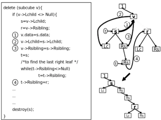
(3) Int. Computer Symposium, Dec. 15-17, 2004, Taipei, Taiwan. 0. 0 2. 5. 4.2. 6. 1 3. 8. add (subcube p, subcube v){. 1. v->Rsibling=p->Lchild; /* p->Lchild maybe a null value */. 3. 7. 4.1. /* p computed v */. 4.1. p->Lchild=v;. 2. }. 4.2. 8. 5. Figure 6: Adding a SDT node algorithm.. 6. 3.5.1. Node Insertion After issuing a new query, if the corresponding subcube is worth materializing, the new subcube fragments are formed and the insertion operation will be performed to insert the new nodes into the SDT for consistency. Figure 5 shows a case that a node is inserted into the SDT. The Node 8 is computed from Node 6, so Node 8 is a child of Node 6 in the SDT. The Node insertion algorithm for the mapped binary tree of SDT is shown in Figure 6. We let the inserted node be the Lchild of its parent node for quicker access in the near future. The operation requires changing only two pointers and thus, the time complexity of the algorithm is O(1).. 7 SDT. Mapped Binary Tree. Figure 3: Transformation of a SDT into a binary tree.. the mapped binary tree. The most popular data structure to represent a binary tree is the linked lists.. 3.4 Node structure The node structure of the SDT transformed binary tree is shown in Figure 4. A node has four parts. Lchild links to the child node, Rsibling links to a sibling node which has the same parent as the node, the block pointer points to the starting address of a disk block that stores the subcube data, and the information field in the node stores the subcube identifier (a combination of subcube cell and subcube class), the dimension value ranges and usage statistics (accessed frequency, last accessed time, etc.). Lchild. Subcube cell. fragment ranges. Subcube class. Usage statistics. Rsibling. 3.5.2. Node deletion Due to the constraints imposed by disk space and update window, the less frequently used subcubes are evicted from the pool of subcubes on disk. The 0. 0 1. 1. 2. 5. 4. 2. 8. 4. 9. 9. 5. 8. Block Pointer. 0. 0 1. Figure 4: Node structure of SDT.. 4. 6 8. 1. 3. s. t. v.data=s.data; v->Rsibling=s->Rsibling;. v 1. r=v->Rsibling;. Lc. Rs. /*to find the last right leaf */. Lc. t=t->Rsibling;. 4. 8 7. …. s Lc. Rs. Rs. …. r. destroy(s); }. Mapped Binary Tree. Rs. 4. 1. t->Rsibling=r;. …. Rs. t. while(t->Rsibling<>Null). 6. r. 3. t=s;. 9 SDT. 2. s=v->Lchild;. 5. 9. 1. if (v->Lchild <> Null){. 2 v->Lchild=s->Lchild;. 4. 7. M a p p e d B in a ry T re e. delete (subcube v){. 2. 4. 8. Figure 7: Deleting a node from SDT.. 1. 5. 4. 9. SDT. 0. 2. 5. 5. The SDT tree is designed for subcube-based query processing. It helps the query processor to search the storage pool for appropriate subcubes. We then explain those algorithms regarding the maintenance of SDT including insertion, deletion and necessary adjustment.. 1. 8. 9. 3.5 Operation algorithms. 0. 1. Lc. Rs. Figure 8: Node deletion algorithm (Case 1).. Figure 5: Inserting a node into the SDT.. 162.

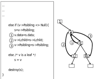
(4) Int. Computer Symposium, Dec. 15-17, 2004, Taipei, Taiwan. /* p computed v */ Add (p,v); Refresh (v); Refresh (subcube v) { s=v; t=v->Rsibling; while (t <> Null) { if (v can compute t) { 1 s->Rsibling=t->Rsibling; 2 t->Rsibling=v->Lchild; 3 v->Lchild=t; 4 t=s->Rsibling; } else { s=s->Rsibling; t=s->Rsibling; } } }. … … … else if (v->Rsibling <> Null){. 1. s=v->Rsibling;. v. 1 v.data=s.data; 2 v->Lchild=s->Lchild; 3 v->Rsibling=s->Rsibling;. 2. else /* v is a leaf */. 3. s. 1. Lc. s=v. Rs. destroy(s); }. p. v. r. p s. v. 1. 3. r. t. 4. 2. p. v. r. Figure 9: Node deletion algorithm (Case 2 & 3).. Figure 11: Adjustment algorithm.. node of an evicted subcube should be deleted from the SDT for consistency. Figure 7 shows a case of deleting a node from SDT. The Node 2 in the SDT is deleted, and its child nodes (Node 4 and Node 8) become child nodes of the parent of Node 2, Node 0. Actually, there are three cases to be considered for the deletion operation of the mapped binary tree: Case 1: v has Lchild. Case 2: v has no Lchild but Rsibling. Case 3: v is a leaf. (The deleted node is assumed to be Node v.) The deletion algorithm for case 1 is shown in Figure 8; for case 2 and case 3 it is shown in Figure 9. The time complexity of the algorithm is O(n), because of the traversal to find the last sibling node in Case 1.. queries, and Node 5 is the parent of both Node 6 and Node 7. However, Node 6 computes Node 7 more efficiently than Node 5 does, so Node 6 is better to be the parent of Node 7 than Node 5. To keep the SDT in the good condition, after inserting a node, the adjustment is necessary be made to discover any potential ancestor-descendant relationship and adjust the SDT accordingly. The adjustment algorithm is proposed in Figure 11. Each node from the Rsibling of the inserted node is checked to the last, so the time complexity of the algorithm is O(n). 3.5.4. Searching The tree, SDT is designed for subcube based query processing. It helps the query processor to search the storage pool for appropriate subcubes. The looking up procedure for nodes is made in breadth-first fashion. At first, the child nodes of the root are checked. If an appropriate node is found, the checking is turned to its child nodes to find the better node. The better of the node is coarser and nearer to the leaf, and more efficiently to compute the query result. By the tree traversal method, the SDT prunes down search space to a subset of potentially appropriate subcubes, as Figure 12 shows.. 3.5.3. Adjustment In the insertion stage of the SDT, an inserted node probably becomes a parent of its sibling. Figure 10 is used as an example to explain it. Nodes 5, 6 and 7 show the ancestor-descendant relationship. When Node 6 is deleted, Node 7 replaces Node 6 and becomes a child of Node 5. After some time, Node 6 may be recomputed from Node 5 for some coming 0. 0. 5. Searching Space. 5. Delete Node 6. N. 6. 7. N. N. Y. 7 Add Node 6. 5 6. Refreshing. Y. Y. 0. 0. N. N. Y N. Y. N. 5 6. N SDT. 7. 7. Y Mapped Binary Tree. Figure 10: An example of adjustment.. Figure 12: Looking up nodes.. 163.

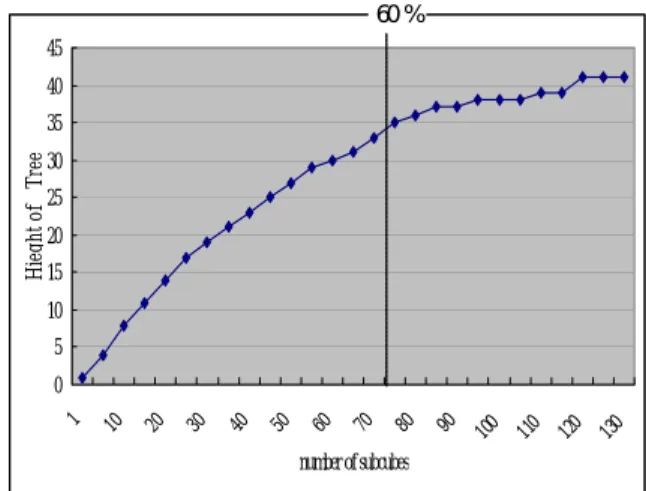
(5) Int. Computer Symposium, Dec. 15-17, 2004, Taipei, Taiwan.. We use the APB-1 OLAP Benchmark File Generator to produce the sample data. [6] The common parameters are: channel=10, number of users= 100. The density is 1.0. The complete relation schemas of the APB-1 Benchmark database are listed below (the subscripts denote corresponding dimension level numbers).. /* Searching a subcube in a SDT */ SDT_Search(SDT t, query cell q) { /* picked node records the recent useful subcube*/ Picked_Node=Null; /*The Lchild of SDT root is the first node being checked */ v=t.Root->Lchild While (v<>Null) if (v can compute q){ Picked_Node=v; v=v->Lchild; } else v=v->Rsibling; } Return Picked_Node; }. SalesFact(Code, Store, Store, Month, UnitsSold, DollarSales) ProdDim(Code7, Class6, Group5, Family4, Line3, Division2, Top1) CustDim(Store3, Retailer2, Top1) ChanDim(Base2, Top1) TimeDim(Month3, Quarter2, Year1). Figure 13: A SDT searching algorithm.. The queries are produced from four types(only these queries are considered directly related to our Sales cube). The query types are listed bellow. Query 1: (?product, ?customer, ?channel, ?time) Query 2: (?product, ?customer, ?channel, ?time) Query3: (?product, ?customer, ?channel, 1995Q11996Q2) divided into two query cells: (?product, ?customer, ?channel, 1995Q1) (?product, ?customer, ?channel, 1996Q1) Query 4:(?product, ?customer, allchannel, ?time). Figure 13 is the searching algorithm for the mapped binary tree. The time complexity of the algorithm is O(n) where n is the number of nodes in the unbalanced binary tree.. 4. Implementation The overall system framework proposed by [5] is shown in Figure 14. The subcubes are stored in the subcube pool. Through the API calls, the subcubes could be accessed, managed and updated by queryPool(), storePool(), and updatePool(), respectively. Our implementation is the queryPool(). updatePool (d). In our implementation, we materialized all the mapped subcubes that we used in the process of computing the query results, and the query values were generated randomly within a range of locality. The height of the mapped binary tree of SDT means the worst case to search a subcube. If the height of the tree is h (including the root), it is possible to search an appropriate subcube by checking h times (h-1 nodes and 1 Null). That is the reason why we concern with the growth of the tree height.. Directory. queryPool (q) storePool (f). 4.2 Results. Pool API. View Pool. 60% 45 40. Hieght of Tree. 35. Figure 14: The overall system framework. including the subcube based query processing algorithm. We implement the algorithm using STM and SDT, respectively.. 30 25 20 15 10 5. 4.1 Environments. 90. 80. 70. 60. 50. 40. 30. 20. 10 0 11 0 12 0 13 0. The system used is a Pentium 4 2.8G Hz with 1GB DDR 400 SDRAM, running Microsoft Windows 2000 Advanced Server and SQL Server 2000. The algorithms were implemented by Microsoft C#.NET.. 10. 1. 0. number of subcubes. Figure 15: The tree height vs. number of subcubes.. 164.

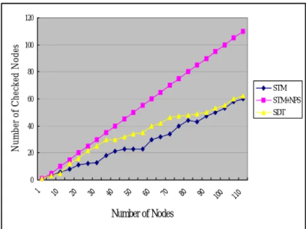
(6) Int. Computer Symposium, Dec. 15-17, 2004, Taipei, Taiwan.. Nearest Sibling) to transform the SDT into the mapped binary tree. The mapped binary tree is therefore like a decision tree for checking whether the subcube is appropriate or not. We design the node structure to store the necessary information and links (Lchild and Rsibling) for a subcube fragment. The necessary management algorithms for insertion, deletion, and adjustment of nodes are also proposed. In our implementation, the SDT shows the efficiency for OLAP queries compared with STM especially when the queries focus on domain ranges (locality property).The other two functions (storePool() and updatePool()) of the system framework in Figure 14 are possible future works. The design of admission of materializing subcubes is an important issue. The storePool() should judge whether the subcube mapped by the new queries is worth materializing or not. The less useful subcubes should be evicted from the pool for the better usage of resources. Once updates occur in base fact table, how to determine those affected subcubes and propagate necessary updates is another issue worth future investigation. updatePool() should adopt a suitable update policy in the update phase.. Number of Checked Nodes. 120 100 80. STM STM+NPS SDT. 60 40 20. 11 0. 90. 10 0. 80. 70. 60. 50. 40. 30. 20. 1. 10. 0. Number of Nodes. Figure 16: Performance comparison. Figure 15 shows that the height of the tree grows with the number of materialized subcubes and the speed of growth is getting slower. When the disk space of materialized subcubes is under 60%, most new nodes are the sibling of existing nodes. After the materialized subcubes occupy 60% of disk space, the growth rate (added height / new nodes) is getting slower (≤ 2 / 5) because the descendant subcubes can be already computed from the existed subcubes. Thus, the newly inserted Lchild nodes do not make the tree much higher. The tree is efficient for looking up when the number of subcubes is large in a specified disk space (the locality property). In the next implementations, the following three algorithms are employed in the query processing: STM: Looking up subcubes in a table stored subcubes' information. When an appropriate is found, it stops searching. STM+NPS: Scanning all records in the STM table for the nearest parent subcube (NPS). SDT: The subcube Dependency Tree. The results show that when the number of subcubes is large (over 60% in our experiments), the spent time in SDT is nearly the same as STM, and SDT found the best subcube spent almost half of the time compared with STM+NPS, as shown in Figure 16. SDT is more efficient than STM+NPS. We also observe that the SDT is nearly a balanced tree when the number of subcubes is large.. Acknowledgement This work has been partially sponsored by the National Science Council under grants NSC93-2213E-036-007.. References [1] H.H. Chen and K.W. Ho, "Implementing Data Cubes via Subcubes," In IDEAS, pp. 378-386, Coimbra, Portugal, 2004. [2] Y. Feng and S. Wang, "Compressed data cube for approximate OLAP query processing,” Journal of Computer Science and Technology, pp. 625-635, May 2002. [3] J. Gray, A. Bosworth, A. Layman, and H. Pirahesh, “Data Cube: A Relational Aggregation Operator Generalizing Group By, Cross-Tab, and Sub-Totals”, In ICDE, pp. 152-159, New Orleans, USA, 1996. [4] V. Harinarayam, A. Rajaraman, and J.D. Ullman, “Implementing Data Cubes Efficiently”, In SIGMOD, pp. 205-216, Montreal, Canada, 1996. [5] Y. Kotidis and N. Roussopoulos, "A Case for Dynamic View Management," ACM Transactions on Database System, Vol. 26, No. 4, pp. 388-423, Dec. 2001. [6] OLAP Council, “OLAP Council APB-1 Benchmark Specification”, White Paper, 1998, available at http://www.olapcouncil.org/research/bmarkly.htm. [7] J.R. Smith, C.S. Li and A. Jhingran, “A Wavelet Framework for Adapting Data Cube Views for OLAP”, IEEE Transactions on Knowledge and Data Engineering, Vol. 16, No. 5, pp.552-565, May 2004. [8] H. Uchiyama, K. Runapongsa and T.J. Teorey, "A Progressive View Materialization Algorithm," In DOLAP, Kansas City, USA, 1999.. 5. Conclusions and Future works By introducing the computational dependency of the data cube lattice framework, we propose the Subcube Dependency Tree (SDT), an improved dictionary to keep the parent-child relationship of subcube fragments. The SDT can prune the search space to save the checking time for the most appropriate subcubes. For storing the SDT with unlimited node degrees (the number of children), we adopt the common method (Left Most Child Right. 165.

(7)