A Fault-tolerant Dynamic Task Scheduling Algorithm for Real-time Systems on Heterogeneous Multiprocessor

全文

(1)Int. Computer Symposium, Dec. 15-17, 2004, Taipei, Taiwan.. A Fault-tolerant Dynamic Task Scheduling Algorithm for Real-time Systems on Heterogeneous Multiprocessor Ming-Dien Chang, Yi-Hsuan Lee, Wen-Pin Liu, and Cheng Chen Department of Computer Science and Information Engineering 1001 Ta Hsueh Road, Hsinchu, Taiwan, 30050, Republic of China Tel: (8863) 5712121 EXT: 54734, Fax: (8863) 5724176 E-mail: {mdchang, yslee, wpliu, cchen}@csie.nctu.edu.tw scheduling, we choose the primary/backup (PB). Abstract Real-time Systems are being increasingly used in. scheme which is the most popular one.. several applications which are time critical. Tasks. Some effective scheduling algorithms used for. corresponding to these applications have deadlines to. real-time multiprocessor system have been proposed. be met. Fault-tolerance is an important requirement. [1-2]. Most of them are designed for homogeneous. of such systems, due to the catastrophic consequences. system, and we have enhanced them to heterogeneous. of not tolerating faults. In this paper, we propose. multiprocessor [8]. In these algorithms, tasks with. density first with minimum non-overlap scheduling. earlier deadlines will be given higher scheduling. algorithm (DNA), which schedule real-time tasks. priorities. However, a task with smaller schedulable. dynamically with primary/backup (PB) scheme on. interval should be schedule early to decrease the. heterogeneous multiprocessor. In DNA we define a. reject ratio. Thus, in our density first with minimum. heuristic function density to prioritize tasks. Besides,. non-overlap scheduling algorithm (DNA), tasks are. we also propose minimum non-overlap (MNO). prioritized with a new heuristic function density.. mechanism for backup scheduling. According to our. Furthermore, we also propose minimum non-overlap. simulations, DNA can achieve higher guarantee ratio. (MNO) mechanism for backup scheduling, which can. in any environment compared with related methods.. minimize the reserved time intervals for backups. Based on simulation results, DNA can achieve higher. 1. Introduction. guarantee ratio in any environment compare with. Real-time systems are defined as those systems in. other related methods.. which its correctness depends not only on the logical. The remainder of this paper is organized as. result of computation, but also on the time at which. follows. Section 2 describes the system model and. the results are produced [1-3]. It can be broadly. related work. Design issues and principles of DNA. classified into three categories [4]. Among them the. are introduced in Section 3. In Section 4, some. hard real-time system is strictest, and in this paper we. experimental results are given. Finally, we give some. will focus on it.. conclusions in Section 5.. Due to the critical nature of tasks in a hard real-time. system,. fault-tolerance. becomes. an. 2. important issue [1-2]. In multiprocessor systems,. 2.1. Fundamental Background System, Task, and Fault Models [1-2]. fault-tolerance can be provided by scheduling. The heterogeneous multiprocessor consists of m. multiple versions of tasks on different processors. processors P1…Pm connected by a network. Every. [5-6]. Among different schemes for fault-tolerant. processor may fail due to hardware or software failure.. 1374.

(2) Int. Computer Symposium, Dec. 15-17, 2004, Taipei, Taiwan. The faults are independent, and only occur in one. of tasks being scheduled, which can lead to select the. processor at a time.. most appropriate task. Moreover, DMA has the. Real-rime task scheduling algorithms usually. capability of backtracking. If the current schedule. assume that tasks are independent, because [8] have. cannot be extended any more, it will deallocate the. proven that precedence constraints can be actually. last scheduled task and try to schedule another one.. removed. Thus, we simply assume tasks are aperiodic,. In [7], we extend DMA to heterogeneous. independent, non-preemptive, and not parallelizable.. multiprocessor and propose heterogeneous distance. Every task Ti has following attributes: ready time (ri),. myopic algorithm (HDMA). Besides, we also design. computation time on processor Pj (cij), and deadline. fault-tolerant myopic algorithm (FTMA), which is. (di). Each task Ti has primary (Pri) and backup (Bki). modified from HDMA [7]. In FTMA, primaries and. copies with identical attributes. Since tasks are not. backups are ordered in separate task queues. In each. parallelizable, di – ri should be long enough to. scheduling step, the first primary or backup with. schedule both primary and backup copies of Ti.. smaller heuristic value will be moved into the. In dynamic multiprocessor scheduling, all tasks. feasibility check window. Compared with HDMA,. arrive at a central scheduler and execute on other. FTMA can select more appropriate tasks to schedule. processors. The scheduler runs in parallel with other. every step. Thus, from simulation results, FTMA. processors, and periodically schedules newly arriving. exactly outperforms HDMA in any environment.. tasks with a small time quantum or as a task arrive. Simply, we assume the scheduler is fault free. 2.2. 3. Related Work. Density First with Minimum Non-overlap Scheduling Algorithm (DNA). Because PB scheme schedules two copies of a. In the first two subsections, we will introduce a. task on different processors, the entire schedulability. new heuristic function density and the minimum. is obviously decreased. Therefore, BB-overloading. non-overlap (MNO) mechanism respectively. The. technique, proposed in [1], describes that Bki and Bkj. overall scheduling steps of our density first with. scheduled on the same processor can be overlapped if. minimum non-overlap scheduling algorithm (DNA). Pri and Prj are scheduled on different processors.. will be listed in Section 3.3.. Backup deallocation reclaims resources reserved for. 3.1. Density Heuristic Function. backups when their corresponding primaries complete. As mentioned above, almost all previous methods. successfully, which is another technique to increase. use deadline to prioritize tasks. However, in order to. the entire schedulability [1].. decrease the reject ratio, a task with smaller. Distance myopic algorithm (DMA) is a heuristic. schedulable interval seems much urgent to be. search algorithm that schedules real-time tasks on. schedule first. We define a density heuristic function,. homogeneous multiprocessor with fault-tolerant [2].. which gives higher priorities for urgent tasks.. It treats Pri and Bki of task Ti as separate tasks and. Definition 3.1 For a task Ti, the latest finish time of. constructs a task queue according to deadlines and. primary (LFP) is defined as LFP (Ti) = di – min {cij}. variable distance. DMA contains two features doing. (1). scheduling. The first one is using a feasibility check. Definition 3.2 For a task Ti, ESTj (Pri) indicates the. window (with size K) to achieve look-ahead nature.. earliest start time of its primary on processor Pj.. The second one is to use an integrated heuristic. ESTj (Pri) = max {ri, avail (j)}, where avail (j) is. function to select task. It will rearrange the sequence. the time that Pj is available to execute Pri. 1375. (2).

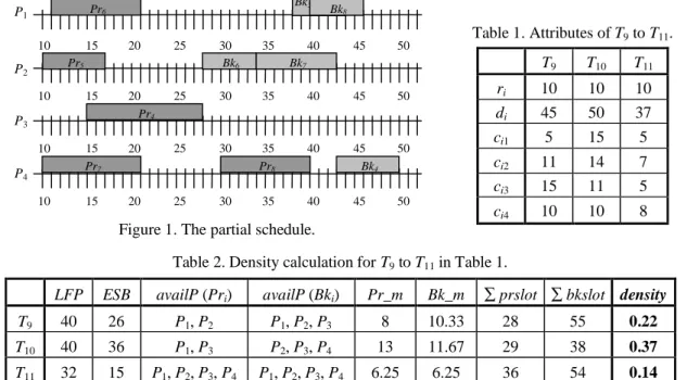
(3) Int. Computer Symposium, Dec. 15-17, 2004, Taipei, Taiwan. Bk5. Pr6. P1. 15. 10. 20. 25. Pr5. P2. 30 Bk6. 35. Bk8. 40. 45. 15. 20 Pr4. 25. 30. 35. 40. 45. 50. 10. 15 Pr7. 20. 25. 30. 35 Pr8. 40. 45 Bk4. 50. 15. 20. 35. 40. 45. 50. P4 10. 25. T9. T10. T11. ri di. 10 45. 10 50. 10 37. ci1. 5. 15. 5. ci2 ci3. 11 15. 14 11. 7 5. ci4. 10. 10. 8. Bk7. 10. P3. Table 1. Attributes of T9 to T11.. 50. 30. Figure 1. The partial schedule. Table 2. Density calculation for T9 to T11 in Table 1. ∑ prslot ∑ bkslot density. LFP. ESB. availP (Pri). availP (Bki). Pr_m. Bk_m. T9. 40. 26. P1, P2. P1, P2, P3. 8. 10.33. 28. 55. 0.22. T10. 40. 36. P1, P3. P2, P3, P4. 13. 11.67. 29. 38. 0.37. T11. 32. 15. P1, P2, P3, P4. P1, P2, P3, P4. 6.25. 6.25. 36. 54. 0.14. Definition 3.3 For a task Ti, the earliest finish time of. density (T i ) =. primary (EFP) is defined as EFT (Ti) = min {ESTj (Pri) + cij}. Pr _ m (Ti ) + Bk _ m (T i ) (7) ∑ prslot ij + ∑ Bkslot ij. j∈availP ( Pr i ). (3). We assume that Bki should be started after Pri. j∈availP ( B ki ). For example, Figure 1 and Table l contains a. finishes, hence, the earliest start time of backup (ESB). partial schedule and attributes of task T9 to T11. Table. is defined as. 2 lists all variables defined above of T9 to T11.. ESB (Ti) = EFP (Ti). (4). Definition 3.4 For a task Ti, availP (Pri) contains all. 3.2. Minimum Non-overlap (MNO) Mechanism. processors that can execute Pri between ri and LFP. In PB scheme, both primary and backup must be. (Ti) without overlapping with scheduled primaries. scheduled before deadline to tolerant processor failure.. and backups.. However, the time intervals reserved for backups are. Definition 3.5 For a task Ti, availP (Bki) contains all. redundant if their primaries finish successfully. Thus,. processors that can execute Bki between ESB (Ti) and. minimizing processor time occupied by backups is an. di without overlapping with scheduled backups.. issue for increasing schedulability.. Definition 3.6 For a processor Pj, prslotij and bkslotij. In other algorithms, backup usually be scheduled. are lengths of time interval on it which can. ALAP or overlapped with other scheduled backups. successfully execute Pri and Bki respectively.. (primaries) as much as possible. Because computation. Definition 3.7 For a task Ti, Pr_m (Ti) and Bk_m (Ti). times of a task on heterogeneous processors are. indicate the average computation time of Pri and Bki. different, maximizing the overlapped time intervals. on availP (Pri) and availP (Bki) respectively.. may still occupy longer non-overlapped intervals.. Pr_m (T i ) =. ∑c. ij. availP ( Pr i ). (5). j∈ availP ( Pr i ). Bk_m (T i ) =. ∑c. ij. Therefore, we propose minimum non-overlap (MNO) mechanism for backup scheduling, which minimizes. availP ( B k i ). (6). j∈ availP ( B k i ). non-overlap time intervals to reserve much time for unscheduled tasks. For example, from Table 2, we. Definition 3.8 For a task Ti, we define its density. select T10 to schedule because it has the maximum. heuristic function as follows:. density. After scheduling Pr10 to P1 in time interval. 1376.

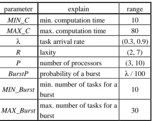
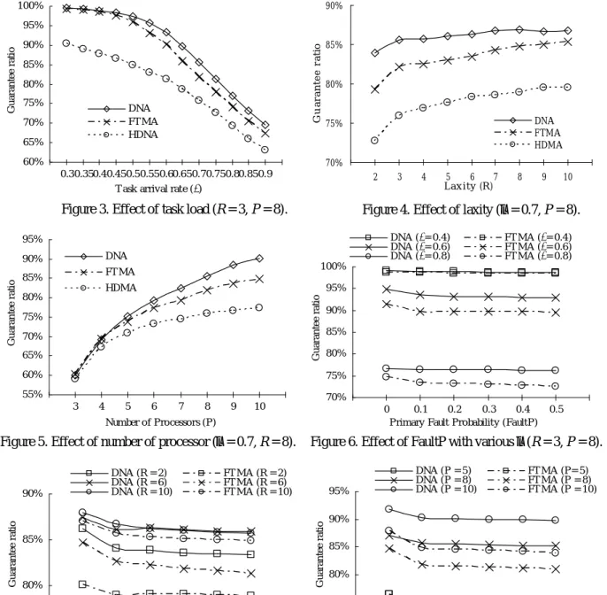
(4) Int. Computer Symposium, Dec. 15-17, 2004, Taipei, Taiwan. 1. Calculate the density heuristic values for all tasks initially 2. (a) Select Ti with the maximum density heuristic value (b) Schedule Pri by EFT (c) if (Pri is scheduled successfully) Schedule Bki by MNO mechanism if (Bki is scheduled successfully) Modify heuristic values of tasks else Deallocate Pri and reject Ti else Reject Ti 3. Repeat Step 2 until all tasks are scheduled. Table 3 lists parameters used in the task generator, which can generate task set with any characteristic. The computation times of a task are chosen uniformly between (MIN_C, MIN_C + (MAX_C – MIN_C) × h), where h is the heterogeneity of computation times of a task. The inter-arrival times between tasks is exponentially distributed with mean (MIN_C + MAX_C) / 2λP [2]. We also simulate bursts of tasks, which the mean of inter-arrival times becomes MIN_C / 10λP. In order to make sure that both copies. Figure 2. The scheduling steps of DNA.. can be successfully scheduled, the deadline of task Ti. (21, 36), Bk10 can be scheduled to P2 in (36, 50), or to. is chosen uniformly between (ri + max cij + second. P3 in (36, 47), or to P4 in (40, 50). Lengths of. max cij, ri + R × max cij).. non-overlap time intervals on P2 to P4 are 7, 11, and 3. We construct a discrete-event dynamic scheduler,. respectively. Hence, Bk10 will be scheduled to P4.. which simulates events including task arrivals, task. 3.3. starts and completions, start of scheduling, backup. DNA Algorithm After introducing heuristic function density and. deallocations, and occurrences of fault. The failure. MNO mechanism, Figure 2 contains the scheduling. may be due to hardware or software. A software fault. steps of our DNA algorithm. Different from three. terminates the task that causes the fault immediately,. methods mentioned in Section 2.2, DNA schedules. and the hardware fault caused by processor failure. both copies of a task simultaneously. This feature. may be permanent or transient. The failed processor. makes DNA more efficient, because it avoids the. with permanent fault will never be available, and will. reconstructing of task queues, the checking of strong. be available after MAX_Recovery if the fault is. feasibility, and backtracking. Notices that either. transient. Related parameters and probabilities for. primary or backup of a task cannot be successfully. failure events are listed in Table 4.. scheduled, the task should be rejected.. 4.2. 2. Experimental Results. The complexity of DNA is O (n ), where n is the. In this subsection, we evaluate performances of. number of tasks in the task queue. Since our central. DNA, HDMA, and FTMA. The total number of tasks. scheduler schedules newly arriving tasks periodically. is 20,000, and 20 task sets are generated for each set. with a small time quantum or as a task arrive, we. of parameters. Because HDMA and FTMA require. believe that n shall not be very large.. additional variables K and distance, we evaluate them with various K and distance combinations and select. 4 4.1. the best result. As for the objective, we use the. Performance Studies. guarantee ratio (GR) defined below that means the. Simulation Environment We construct a dynamic simulation environment. to evaluate DNA. It contains two parts named task. percentage of tasks whose deadlines are met [9]. GR =. generator and scheduler, and we describe them in. number of tasks whose deadlines are met ×100% (8) total number of tasks arrived in the system. With fixed probability of primary fails (FaultP. detail in the following. The task generator generates a set of real-time. =0.2), Figures 3~5 show results of various task arrival. tasks in the non-decreasing order of ready times.. rate, laxity, and number of processors, respectively.. 1377.

(5) Int. Computer Symposium, Dec. 15-17, 2004, Taipei, Taiwan. Table 3. Parameters for task generator. parameter. explain. Table 4. Parameters for fault probability.. range. parameter. MIN_C MAX_C λ R P BurstP. min. computation time 10 max. computation time 80 task arrival rate (0.3, 0.9) laxity (2, 7) number of processors (3, 10) probability of a burst λ / 100 min. number of tasks for a 10 MIN_Burst burst max. number of tasks for a MAX_Burst 30 burst. explain. range. probability that a primary (0, 0.5) fails probability that a primary Soft_FP 0.2 fails due to software fault probability that a primary Hard_FP 0.8 fails due to hardware fault probability that a hard10-6 PermHard_FP ware fault is permanent FaultP. MAX_Recovery. max. recovery time after a transient hardware fault. 50. These results clearly indicate that DNA outperforms. quite efficient, which is appropriate to be used in. HDMA and FTMA, which means using the density. real-time systems.. heuristic function can select more appropriate tasks to schedule at each scheduling step. Meanwhile, the GR. Reference. is higher with lower λ, larger R, and larger P. The. [1] S. Ghosh, R. Melhem, and D. Mosse, “Fault-. reason of lower λ and larger R seems trivially. As for. tolerance Through Scheduling of Aperiodic Tasks. larger P, using MNO mechanism will schedule. in Hard Real-time Multiprocessor Systems”,. backups as tight as possible, so more time intervals. IEEE Trans. on Parallel and Distributed Systems,. can be reserved for primaries when P is larger.. Vol. 8, No. 3, pp. 272-284, March 1997.. In Figures 6~8, the probability of primary fails is. [2] G. Manimaran and C. S. M. Murthy, “A Fault-. varied with parameters λ, R, and P. While the fault. tolerant Dynamic Scheduling Algorithm for Mul-. probability increases, more backups are active to be. tiprocessor Real-time Systems and Its Analysis”,. executed. So, less time intervals reserved for backups. IEEE Trans. on Parallel and Distributed Systems,. can be reutilized, which decreases the entire GR. In. Vol. 9, No. 11, pp. 1137-1152, Nov. 1998.. these results, DNA still has higher GR than that of. [3] K.. Ramamritham. and. J.. A.. Stankovic,. FTMA in any simulation environment. That is to say,. “Scheduling Algorithms and Operating Systems. our DNA is not only an efficient algorithm, but also. Support for Real-time Systems”, Proc. of IEEE,. quite effective compared with related methods.. Vol. 82, No. 1, pp. 55-67, Jan. 1994. [4] K. G. Shin and P. Ramanathan, “Real-time. 5. Concluding Remarks. Computing: A New Discipline of Computer. In this paper, we propose a fault-tolerant dynamic. Science and Engineering”, Proc. of IEEE, Vol. 82,. task scheduling algorithm DNA for real-time systems. No. 1, pp. 6-24, Jan. 1994.. on heterogeneous multiprocessor. In DNA we design. [5] A. L. Liestman and R. H. Campbell, “A. density heuristic function and MNO mechanism,. Fault-tolerant Scheduling Problem”, IEEE Trans.. which are used for task prioritizing and backup. on Software Engineering, Vol. 12, No. 11, pp.. scheduling. According to our simulation results, DNA. 1089-1095, Nov. 1988.. achieves higher guarantee ratio than other related. [6] Y. Oh and S. Son, “Multiprocessor Support for. methods in any simulation environment. Besides, it is. Real-time Fault-tolerant Scheduling”, Proc. of. 1378.

(6) Int. Computer Symposium, Dec. 15-17, 2004, Taipei, Taiwan. 90%. 100%. 90%. Guarantee ratio. Guarantee ratio. 95%. 85% 80% 75%. DNA FTMA HDNA. 70% 65%. 85%. 80%. DNA FTMA HDMA. 75%. 70%. 60% 0.30.350.40.450.50.550.60.650.70.750.80.850.9 T ask arrival rate (λ). 2. Figure 3. Effect of task load (R = 3, P = 8).. 3. DNA (λ= 0.4) DNA (λ= 0.6) DNA (λ= 0.8). DNA. 9. 10. FT MA (λ= 0.4) FT MA (λ= 0.6) FT MA (λ= 0.8). 95% Guarantee ratio. Guarantee ratio. HDMA 80% 75% 70% 65% 60%. 90% 85% 80% 75%. 55%. 70% 3. 4. 5. 6. 7. 8. 9. 10. 0. Number of Processors (P). Figure 5. Effect of number of processor (λ = 0.7, R = 8). DNA (R = 2) DNA (R = 6) DNA (R = 10). 0.1 0.2 0.3 0.4 P rimary Fault Probability (FaultP). 0.5. Figure 6. Effect of FaultP with various λ (R = 3, P = 8).. FT MA (R = 2) FT MA (R = 6) FT MA (R = 10). DNA (P = 5) DNA (P = 8) DNA (P = 10). 95%. Guarantee ratio. 90% Guarantee ratio. 8. 100%. FT MA. 85%. 5 6 7 Laxity (R). Figure 4. Effect of laxity (λ = 0.7, P = 8).. 95% 90%. 4. 85%. 80%. FT MA (P= 5) FT MA (P = 8) FT MA (P = 10). 90% 85% 80% 75% 70%. 75% 0. 0. 0.1 0.2 0.3 0.4 0.5 Primary Fault Probability (FaultP). 0.1 0.2 0.3 0.4 0.5 Primary Fault P robability (FaultP). Figure 7. Effect of FaultP with various R (λ = 0.7, P = 8). Figure 8. Effect of FaultP with various P (λ = 0.7, R = 3).. IEEE. Workshop. Architectural. Aspects. J. Y. Chung, “Imprecise Computations”, Proc. of. of. Real-time Systems, pp. 76-80, Dec. 1991.. IEEE, Vol. 82, No. 1, pp. 83-94, Jan. 1994.. [7] Y. H. Lee and C. Chen, “Effective Fault-tolerant. [9] K. Ramamritham, J. A. Stankovic, and P. -F.. Scheduling Algorithm for Real-time Tasks on. Shiah, “Efficient Scheduling Algorithms for. Heterogeneous Systems”, Proc. of National. Real-time Multiprocessor Systems”, IEEE Trans.. Computer Symposium, Dec. 2003.. on Parallel and Distributed Systems, Vol. 1, No.. [8] J. W. S. Liu, W. K. Shih, K. J. Lin, R. Bettati, and. 1379. 2, pp. 184-194, Apr. 1990..

(7)