用於畫面之間的小波轉換編碼以人類視覺系統為基礎的位元控制法

全文

(1)國立交通大學電子工程學系電子研究所碩士班碩士論文. 用於畫面之間的小波轉換編碼以人類視覺系統為基礎的位元控制法 HVS-based Rate Control Algorithm for Interframe Wavelet Video Coding. 研究生：洪朝雄指導教授：杭學鳴博士中華民國九十四年六月.

(2) 用於畫面之間的小波轉換編碼以人類視覺系統為基礎的位元控制法 HVS-based Rate Control Algorithm for Interframe Wavelet Video Coding. 研究生：洪朝雄指導教授：杭學鳴博士. Student: Chao-Hsiung Hong Advisor: Dr. Hsueh-Ming Hang. 國立交通大學電子工程學系電子研究所碩士班碩士論文. A Thesis Submitted to the Institute of Electronics College of Electrical Engineering and Computer Science National Chiao Tung University in Partial Fulfillment of Requirements for the Degree of Master of Science in Electronics Engineering June 2005 Hsinchu, Taiwan, Republic of China. 中華民國九十四年六月.

(3) 用於畫面之間的小波轉換編碼以人類視覺系統為基礎的位元控制法. 研究生：洪朝雄. 指導教授：杭學鳴. 國立交通大學電子工程學系電子研究所碩士班. 摘要因為在大多數的應用中，不同的接收者會有不同的承受量，故可調整性 (scalability)在今天的多媒體傳輸中是一個重要的特性。用於畫面之間的小波轉換編碼(Interframe Wavelet Video Coding)是一個新的視訊編碼方式且能提供良好的可調整性。因此這個編碼方式在近年來受到不少矚目，而且已經有很多的研究和改良來增進它的效能。在很多環境下，人眼都是視訊品質的最後判斷所在。然而，在設計視訊編碼時要包含人類視覺卻很困難。我們必須要能把客觀的“數學上的不同＂轉換成主觀的“視覺上的不同＂，也就是說，我們必須要把普通的“量化錯誤＂轉換成 “人類視覺上的加重錯誤＂。在位元控制法(rate control algorithm)中，每個在用於畫面之間的小波轉換編碼的截斷點(truncation point)都有自己相關聯的失真(distortion)和位元長度(bits length)。而每個截斷點的斜率(slope)就是把失真的差異(distortion difference)除以位元差異(bit difference)所得到的商。在最佳化理論中(optimization theory)，擁有較高斜率的截斷點有較高的優先權被傳送。在本論文中，我們提出一個方法，就是說我們把每個截斷點的斜率乘上一個由人類視覺系統算出來的比重。故這個經過視覺加重的斜率會成為位元控制法中判斷的標準。我們的模擬會指出最後的重建影像有較低的最高訊號雜訊比(PSNR)和較佳的視覺品質。 i.

(4) HVS-based Rate Control Algorithm for Interframe Wavelet Video Coding Student: Chao-Hsiung Hong. Advisor: Dr. Hsueh-Ming Hang. Department of Electronics Engineering & Institute of Electronics National Chiao Tung University. Abstract Scalability is an important feature in today’s multimedia transmission because in many applications receivers have very different capabilities. Interframe wavelet video coding is a new video coding algorithm that can achieve fine-scale scalability. Therefore, it has received a lot of attention recently and many research and development projects have been conducted to improve its performance. For most entertainment purposes, human eyes are the final judge of the video quality. However, it is rather sophisticated to include the human perception in the video codec design. We need to transform the objective “mathematical difference” into the subjective “visual difference”, i.e., we need to convert the ordinary “quantization error” to the “human-visual weighted error”. In the rate control algorithm, each truncation point in the interframe wavelet video coding has its associated distortion and bits length. The slope of each truncation point is the quotient of the distortion difference divided by the bit difference. Based on the optimization theory, the truncation point with a larger slope should have a higher priority to transmit. In this study, we propose a method that we weight the truncation point slope by a weighting factor, which is derived based on the human visual system. Thus, the visually-weighted slopes become the criterion in rate control. Our simulations indicate that the reconstructed frames may have lower PSNR but higher visual quality. ii.

(5) 誌謝感謝杭學鳴老師，這兩年不厭其煩地指導我，讓我漸漸學習到如何作研究以及作研究該注意的事。再來要感謝我的家人。謝謝我父母和我哥哥總是在背後支持我和給我許多地鼓勵。還有謝謝實驗室裡的許多的學長姐和同學，大家給了我許多研究方面的建議，還有實驗室優良的環境，讓我可以好好地從事研究工作。經過了兩年的研究生活，雖然中間碰過不少困難，不過感謝大家的幫忙，讓我能完成我的學業。在此把這本論文獻給所有幫助過我的人和我所感謝的人。. iii.

(6) Contents 摘要.........................................................................................................................i Abstract ..................................................................................................................ii 誌謝...................................................................................................................... iii Contents ................................................................................................................iv List of Figures ......................................................................................................vii List of Tables.........................................................................................................xi Chapter 1 Introduction ...........................................................................................1 Chapter 2 Scalable Video Coding ..........................................................................3 2.1 Introduction..............................................................................................3 2.2 Subband Video Coding ............................................................................4 2.2.1 Temporal Subband Decomposition...............................................6 2.2.2 Spatial Subband Decomposition ...................................................9 2.2.3 Coding.........................................................................................10 2.3 Interframe Wavelet Video Coding .........................................................10 2.3.1 Introduction.................................................................................10 2.3.2 Motion Compensation Temporal Filtering..................................12 2.3.3 Spatial Analysis...........................................................................18 2.3.4 Embedded ZeroBlock Coding.....................................................19 2.3.5 Entropy Coding...........................................................................20 2.4 Scalable Video Coding...........................................................................21 2.4.1 Rate/SNR Scalability ..................................................................22 2.4.2 Spatial Scalability .......................................................................23 iv.

(7) 2.4.3 Temporal Scalability ...................................................................24 Chapter 3 3D Subband Video Coding Using Barbell Lifting ..............................26 3.1 Barbell Lifting........................................................................................26 3.1.1 The Prediction Stage ...................................................................28 3.1.2 The Update Stage ........................................................................29 3.2 Spatial Decomposition ...........................................................................31 3.3 Multi-Layer Motion Estimation and Coding .........................................32 3.4 3D ESCOT .............................................................................................32 3.4.1 Zero Coding ................................................................................33 3.4.2 Sign Coding ................................................................................35 3.4.3 Magnitude Refinement................................................................36 3.4.4 Fractional Bit-Plane Coding .......................................................36 3.5 Bitstream Truncation and Scalability.....................................................37 Chapter 4 Human Visual System .........................................................................41 4.1 Human Vision ........................................................................................41 4.2 Color Representation .............................................................................43 4.3 Contrast Sensitivity................................................................................45 4.4 Masking Effect.......................................................................................46 4.5 Just-Noticeable Distortion .....................................................................47 Chapter 5 Rate Control Algorithm Based on HVS ..............................................51 5.1 Transform R-D Slope Representation....................................................51 5.2 Weighting Factor....................................................................................52 5.2.1 Intra-Subband Weighting Factor .................................................52 5.2.2 Inter-Subband Weighting Factor .................................................62 5.3 Rate Control ...........................................................................................64 v.

(8) 5.4 Experimental Results .............................................................................64 5.4.1 Correctness of the Proposed Rate Control Algorithm.................64 5.4.2 Comparison of Rate Control Algorithms ....................................78 5.5 Discussion ..............................................................................................88 Chapter 6 Conclusion and Future Work...............................................................89 6.1 Conclusion .............................................................................................89 6.2 Future Work ...........................................................................................90 References............................................................................................................91 作者簡歷..............................................................................................................96. vi.

(9) List of Figures Figure 2-1 Classifications of video coders.....................................................3 Figure 2-2 Typical 3-D subband decomposition............................................5 Figure 2-3 The temporal filtered images using Haar filter (left：low pass, right：high pass)....................................................................................6 Figure 2-4 Temporal filtering with motion compensation (left：low pass, right：high pass)....................................................................................7 Figure 2-5 Vector mismatch caused by moving and zooming objects...........7 Figure 2-6 The spatial lattices of two consecutive frames after motion estimation. The black circle is the pixel being processed. The gray pixels and arrows indicate the direction of filtering. (a)class EO:2dx even and 2dy odd, (b)class OE: 2dx odd and 2dy even, (c)class OO: 2dx odd and 2dy odd, (d)class EE: 2dx even and 2dy even. ..................8 Figure 2- 7 Spatial decomposition (left：transformed image, right：frequency partion)...................................................................................................9 Figure 2-8 The interframe wavelet video coder...........................................11 Figure 2-9 Temporal filtering pyramid. .......................................................12 Figure 2-10 A 3 level HVSBM showing 3 subband levels [13]. .................14 Figure 2-11 State of connection of each pixel [13]......................................15 Figure 2-12 Lifting scheme in temporal filtering. .......................................17 Figure 2-13 Detection of connected and unconnected pixels. .....................17 Figure 2-14 Quad-tree generation of the image [10]. ..................................20 Figure 2-15 Map representation of the quad-tree. .......................................20 Figure 2-16 Motion vector coding scanning trail. .......................................21 vii.

(10) Figure 2-17 The interframe wavelet video coding encoded bitstream.........22 Figure 2-18 Rate/SNR scalability. ...............................................................23 Figure 2-19 Spatial scalability. ....................................................................24 Figure 2-20 Temporal scalability. ................................................................25. Figure 3-1 The block diagram of the 3D subband video coding using Barbell lifting [15]. ..............................................................................26 Figure 3-2 The Barbell lifting [15]. .............................................................27 Figure 3-3 The prediction stage of the Barbell lifting. ................................28 Figure 3-4 The update stage of the Barbell lifting.......................................28 Figure 3-5 The Barbell functions used in the prediction stage. ...................28 Figure 3-6 The mismatch problem of motion in the prediction and update stages....................................................................................................30 Figure 3-7 The frame after 3 level spatial decomposition. ..........................31 Figure 3-8 Multi-layer motion estimation and coding.................................32 Figure 3-9 Four types of coding neighbors for zero coding. .......................34. Figure 4-1 Cross-section of human eye [19]................................................41 Figure 4-2 The process of the visual input signal [21]. ...............................42 Figure 4-3 Relative sensitivity of each photoreceptor [21]. ........................43 Figure 4-4 Operations for calculating the weighted average of luminance changes in four directions. ...................................................................48 Figure 4-5 The operator for calculating the average background luminance. ..............................................................................................................49 Figure 4-6 Error visibility thresholds due to background luminance in the spatial domain [28]. .............................................................................49 viii.

(11) Figure 4-7 Error visibility threshold in the spatial-temporal domain, which is modeled. as a scale factor or interframe luminance difference and. the JND value in the spatial domain [28].............................................50. Figure 5-1 The level, orientation, spatial frequency, and minimum threshold of each..................................................................................................54 Figure 5-2 The contrast masking function. ..................................................55 Figure 5-3 t JND (λ ,θ ,0) of the frame shown in Figure 5-1...........................59 Figure 5-4 The flow chart of calculating the subband weighting factor w. .64 Figure 5-5 The four test frames for comparison of test frame I...................67 Figure 5-6 The truncated coding passes of test frame I. The required bit rate is 4.23M bytes per second if the frame rate is 30 frames/sec. .............68 Figure 5-7 The four test frames for comparison of test frame II. ................70 Figure 5-8 The truncated coding passes of test frame II. The required bit rate is 5.64M bytes per second if the frame rate is 30 frames/sec. ......71 Figure 5-9 The four test frames for comparison of test frame III. ...............73 Figure 5-10 The truncated coding passes of test frame III. The required bit rate is 3.54M bytes per second if the frame rate is 30 frames/sec. ......74 Figure 5-11 The four test frames for comparison of test frame IV. .............76 Figure 5-12 The truncated coding passes of test frame IV. The required bit rate is 4.92M bytes per second if the frame rate is 30 frames/sec. ......77 Figure 5-13 The four test frames of frame I at low bit rates. (a) and (b) are 500K bits per second. (c) and (d) are 1000K bits per second. .............80 Figure 5-14 The four test frames of frame II at low bit rates. (a) and (b) are 500K bits per second. (c) and (d) are 1000K bits per second. .............82 Figure 5-15 The four test frames of frame III at low bit rates. (a) and (b) are ix.

(12) 500K bits per second. (c) and (d) are 1000K bits per second. .............84 Figure 5-16 The four test frames of frame IV at low bit rates. (a) and (b) are 500K bits per second. (c) and (d) are 1000K bits per second. .............87. x.

(13) List of Tables Table 2-1 The coefficients of filters. ............................................................19. Table 3-1 The coefficients of the Daubechies 9/7 analysis filters. ..............32 Table 3-2 Context assignment map for ZC. .................................................35 Table 3-3 Context assignment and sign prediction map for SC...................36. Table 5-1 The coefficients of the Daubechies 9/7 synthesis filters..............58. xi.

(14) Chapter 1 Introduction Digital video compression technology has an explosive growth in the past 20 years. The invention of digital video products, such as VCD and DVD, is due to the advances of the digital compression technology. Owing to the rapid development of the internet transmission, it is also important to transmit the video data through the network. Due to the different network bandwidth and different receiver storage capacity, many methods have been investigated to solve the problem of transmitting the compressed video bitstream through the internet. The concept of “scalability” is one of the methods that solve this problem. The “scalability” means that the bitstream can be truncated and decoded anywhere on the bitstream; thus, we can generate the bitstream only once then truncate it to meet the requirements. However, in a traditional scalable video system, because of the lower compression efficiency and course-step in scalability (typically, 2 or 3 layers), its adaptation is not yet so popular. The new technique of fine-granularity scalability is introduced recently [1]. Ohm proposed a motion-compensated t+2D frequency coding structure [2]. This coding structure is suitable for scalable video coding with many fine steps. Woods proposed a coding technique called “interframe wavelet video coding” [3]. This coding technique can offer fine-granularity SNR, temporal and spatial scalability at the same time, while it still maintains acceptable compression efficiency. The main concept of interframe wavelet video coding is subband coding. It removes the temporal redundancy by using the motion-compensated (wavelet) filtering technique along the temporal axis. Then it uses the spatial wavelet 1.

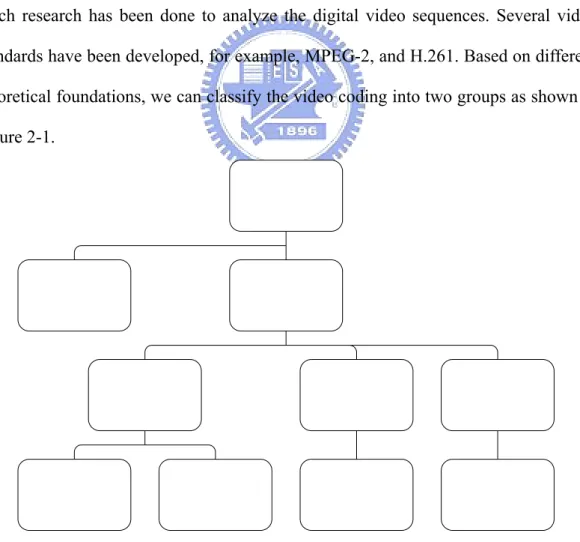
(15) decomposition to the temporal wavelet-filtered output frames. Then we can use the bit-plane coding scheme to code wavelet coefficients and calculate the slope of each fractional bit-plane truncation point to achieve optimal rate control. By this rate control scheme, we can achieve fine-granularity scalability [4]. The quality measure that often be used to determine the quality of images is PSNR. But human eyes have different sensitivity on different regions and frequency bands, the image that has high PSNR value may not have high visual quality. Human eyes usually have higher sensitivity on the low frequency bands and lower sensitivity on the high frequency bands. For the different region, human eyes usually have higher sensitivity in the flat region than in the texture region. We can incorporate human visual system (HVS) to encode each subband to achieve higher visual quality. In this research, we propose a rate control algorithm based on HVS to achieve high visual quality. We apply HVS on spatial frequency and luminance component. There two weighting factors, intra-subband weighting factor and inter-subband weighting factor, that we found will be introduced. The final reconstructed images will have higher visual quality, especially in large flat region. The PSNR of final reconstructed images will be lower. In the future, we will extend this algorithm to temporal frequency and chrominance component. The thesis is organized as follows. In Chapter 2, we will introduce the basic concept and the scalability of scalable video coding. Then we will introduce the program we used in Chapter 3. We will introduce some basic idea of HVS in Chapter 4. The algorithm we developed is introduced in Chapter 5 and Chapter 6 is the conclusion and future work.. 2.

(16) Chapter 2 Scalable Video Coding 2.1 Introduction Digital Video is now very popular in our daily life. For example, DVD and VCD are all digital video. If the digital video has high quality, it usually has a large amount of data. So it needs large bandwidth to transmit or large space to store. To solve this problem, we need to compress the digital video in order to make its data size smaller. Digital video compression technique has been developed in the past three decades and much research has been done to analyze the digital video sequences. Several video standards have been developed, for example, MPEG-2, and H.261. Based on different theoretical foundations, we can classify the video coding into two groups as shown in Figure 2-1.. Figure 2-1 Classifications of video coders. From Figure 2-1, we can see that video coders can be classified into “model based” 3.

(17) and “signal based” two groups. If the video coding algorithm is based on object modeling and analysis of object parameters, it belongs to model based video coding. Model based video coding algorithms usually need a profound analysis of the video contents and are quite complicated. Because of inefficiency and complexity of video object content analysis, model based video coding algorithms are often not so popular. On the other hand, the signal based video coding algorithms consider the objects as the combination of the set of basic signals. So they often use filters to decompose the video sequences into different basic signals. The signal decomposition of these algorithms has two spatial dimensions (horizontal and vertical) and one temporal dimension. Both spatial and temporal decomposition are used to remove in-between redundancies. We usually use discrete cosine transform (DCT) or discrete wavelet transform (DWT) to do spatial decomposition and motion compensated temporal filtering (MCTF) or motion compensated prediction (MCP) to do temporal decomposition. The motion compensated approaches decompose the source output into different frequency subband using block transforms. But decomposition of the source output into blocks will generate coding artifacts at the block edges called blocking effects. Another approach, which can avoid this blocking artifact, is the subband video coding. The subband video coding transforms the total frame into different subbands in spatial and temporal domain, so it can remove blocking effect.. 2.2 Subband Video Coding Subband video coding uses subband filters to remove the spatial and temporal redundancies of the video sequences. Generally speaking, the behavior of the spatial and temporal signals of a video sequence is quite different. For temporal signal, if something moves fast in the video sequence, then the video sequence has high 4.

(18) frequency temporal signal component. The spatial signal will be only considered in the still image. If a still image has many edges or different luminance component in a small area, then it has high frequency spatial signal component. Spatial signal has 2 dimensions (horizontal and vertical) and temporal signal has 1 dimension, so the decomposition of spatial signal is often done twice. Typical 3-D subband signal decomposition is shown in Figure 2-2.. Figure 2-2 Typical 3-D subband decomposition. After spatial and temporal decomposition, the data are sent to quantize and coding. After coding, the coded data is packaged and transmitted to the receiver to decode. 5.

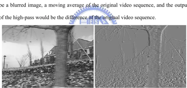
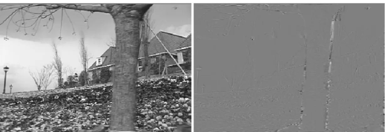
(19) Because human eyes have different sensitivity on different frequency subbands, we can quantize the frequency subbands with higher sensitivity by smaller step size and other frequency subbands by larger step size. Thus we can get the reconstructed video sequence with higher visual quality but lower PSNR value. We will introduce the temporal decomposition and spatial decomposition in next two subsections.. 2.2.1 Temporal Subband Decomposition Temporal subband decomposition can be simply done by use a low pass filter and a high pass filter along the temporal axis. The filter used more often is Haar filter. But the result is not usually good because the energy is not compacted very well. The result is shown in Figure 2-3. We can see that the output of the low-pass filter would be a blurred image, a moving average of the original video sequence, and the output of the high-pass would be the difference of the original video sequence.. Figure 2-3 The temporal filtered images using Haar filter (left: low pass, right: high pass). Kronander used motion compensated technique to solve this problem [5]. For two consecutive frames, we use forward block motion estimation first and backward block motion estimation second. The forward motion compensated reconstructed frame is then used to do temporal filtering with the second frame to generate subband image. Then the backward motion compensated reconstructed frame is used to do temporal filtering with the first frame. The result frames has better energy compaction as shown 6.

(20) in Figure 2-4. There may be a mismatch between these two vectors and it will cause the spatial inhomogeneity. The mismatch often occurs in the covered and uncovered area on the frame, as shown in Figure 2-5. Figure 2-4 Temporal filtering with motion compensation (left: low pass, right: high pass).. covered. covered. uncovered. uncovered covered. uncovered. Figure 2-5 Vector mismatch caused by moving and zooming objects. Ohm proposed a method to solve the spatial inhomogeneity [2]. He showed that it is possible to overcome the mismatch of motion trajectories by using the concept of connected and unconnected pixels. In the proposed algorithm, each pixel is classified as covered, uncovered or connected by using the information derived from the motion vector map. Then Haar filter is used to do temporal filtering to find the high-pass coefficients and the low-pass coefficients. If the integer pixel accuracy motion estimation is used, this method can achieve perfect reconstruction. 7.

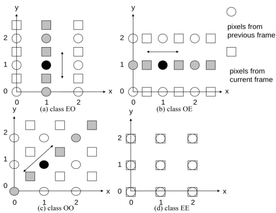
(21) Hsiang and Woods proposed an invertible half-pixel motion estimation three-dimensional analysis/synthesis system for video coding [6]. If we assume that dx and dy are the horizontal and vertical displacement vector between previous and current frames, and they can be pixel or half pixel. Then we can classify the motion compensated blocks into four different kinds, as shown in Figure 2-6. The motion compensated blocks would map to different location of the image, but would lie in horizontal, vertical, diagonal, or overlapped position. Therefore, temporal Haar filtering can be done along those directions to achieve half-pixel-accurate motion estimation. y. y. 2. 2. 1. 1. pixels from previous frame. pixels from current frame 0. x 0 y. 0. x 0 y. 1 2 (a) class EO. 2. 1 2 (b) class OE. 2. 1. 1. 0. x 0. 1 2 (c) class OO. 0. x 0. 1 2 (d) class EE. Figure 2-6 The spatial lattices of two consecutive frames after motion estimation. The black circle is the pixel being processed. The gray pixels and arrows indicate the direction of filtering. (a)class EO:2dx even and 2dy odd, (b)class OE: 2dx odd and 2dy even, (c)class OO: 2dx odd and 2dy odd, (d)class EE: 2dx even and 2dy even. 8.

(22) Pesquet-Popescu and Bottreau proposed a lifting scheme to do temporal filtering [7]. By separating the process of deducting the low-pass and high-pass frequencies, interpolation filters can be used without interfering with the filtering process. Temporal filtering techniques are still being researched and developed. The goal of the temporal filter is make the energy compacted well.. 2.2.2 Spatial Subband Decomposition Spatial decomposition is done along horizontal and vertical directions. The still image is separated into the spatial subband then each subband is encoded independently. The image is reconstructed from the low subband data to high subband data. The major differences are how to choose the analysis and synthesis filters. In other words, that is how to choose the decomposition signal. The performance of the filter will affect the quality of the reconstructed images. The most popular spatial subband decomposition is the wavelet transform. Wavelet transform is a type of localized time-frequency analysis; therefore, the transform coefficients reflect the energy distribution of the source signal in both space and frequency domains. Figure 2- 7 shows an example of the spatial decomposition.. Figure 2- 7 Spatial decomposition (left: transformed image, right: frequency partion). 9.

(23) 2.2.3 Coding Shapiro proposed a coding algorithm called “Embedded image coding using zerotrees of wavelet coefficients (EZW)” [8]. It is a simple but effective coding structure. It arranges the coded data in the order of importance so it is suitable for progressive transmission. Taubman proposed a coding algorithm called “Embedded Block Coding with Optimized Truncation of the embedded bit-stream (EBCOT)” [9]. This is a coding algorithm that JPEG2000 used. It is a fractional bit plane coding and can match the requirement of the rate control. Woods proposed a coding algorithm called “Embedded Zero Block Coding (EZBC)” [10]. It combines the advantages of the zero-tree/-block coding and context modeling of the subband/wavelet coefficients.. 2.3 Interframe Wavelet Video Coding 2.3.1 Introduction The efficient family of interframe wavelet video codecs was proposed by Woods and his coworkers [6] [10] [12] and can achieve rate/SNR, spatial, and temporal scalability. It was first presented by Woods et al for the MPEG digital cinema encoding tool [11]. Many research and development have been made to improve the performance of the interframe wavelet video coder today. In the rest of this thesis, if not specifically stated, the interframe wavelet coding algorithm referred is the latest version proposed by Woods and Chen [12]. The interframe wavelet coder is one kind of motion compensated 3-D subband coder. 3-D is 2 spatial dimensions (horizontal and vertical) and 1 temporal dimension. This coding algorithm is also known as the “Motion Compensated Temporal 10.

(24) Filtering – Embedded Zero Block Coding (MCTF-EZBC or MC-EZBC)”. This coding algorithm uses motion compensated temporal filtering techniques when doing temporal subband decomposition. After temporal subband decomposition, each produced frame is spatially subband decomposed by wavelet transform. After temporal and spatial decomposition, the wavelet coefficient is coded by embedded zeroblock coding techniques [10]. Then we can package and truncate the coded bitstream and transmit it to the receiver and decode. The architecture of the interframe wavelet video coder is shown in Figure 2-8. Input Video. MCTF (analysis). Spatial Analysis. Motion Estimation. Output Video. MCTF (synthesis). EZBC. Packetizer. Encoder. Motion Field Encoding. Spatial Synthesis. EZBC. Depacketi zer. Motion Field Decoding. Decoder. Figure 2-8 The interframe wavelet video coder. The processing unit is GOP (group of pictures) and the frame number of each GOP is 2n, where n is the number of levels of temporal subband decompositions that are done on the GOP. When doing temporal subband decomposition, the motion vector map between two consecutive frames is first constructed. Then motion compensated temporal filtering is applied to the two consecutive frames to generate the temporal high-pass frame and the temporal low-pass frame. After first temporal decomposition, the GOP would contain 2n-1 temporal high-pass frames and 2n-1 temporal low-pass frames. Then 2n-1 temporal low-pass frames would be collected to do temporal decomposition again. These 2n-1 temporal low-pass frames 11.

(25) would transform to 2n-2 temporal high-pass frames and 2n-2 temporal low-pass frames. The temporal decomposition is iteratively done until there is only one temporal low-pass frame. After finishing temporal decomposition, we can get a temporal filtering pyramid as shown in Figure 2-9.. Video Sequence MCTF. GOP (Group of Pictures) Corresponding to temporal level=4 decomposition. MCTF. MCTF. Temporal Low-pass frame Temporal High-pass frame. MCTF. Frames that remain after temporal decomposition. Figure 2-9 Temporal filtering pyramid. After temporal decomposition is done, the 2n frame GOP would contain 2n-1 temporal high-pass frames and one temporal low-pass frame. These frames are called residual frames. The spatial subband decomposition is then applied to each frame to create wavelet coefficients of each spatial subband. The wavelet coefficients is then coded by embedded zeroblock coding method, and then entropy-coded by arithmetic coding with context modeling [10].. 2.3.2 Motion Compensation Temporal Filtering The interframe wavelet video coding uses motion compensated temporal filtering (MCTF) to do temporal subband decomposition and the goal of motion compensated temporal filtering is to compact the video sequence temporal energy. 12.

(26) The first step of MCTF is motion estimation and there two things need to do in this step. First is using “hierarchical variable size block matching (HVSBM)” to do backward motion estimation. Second is detecting covered and uncovered pixels based on the backward motion field [13].. 2.3.2.1 Hierarchical Variable Block Size Matching HVSBM is a hierarchical motion estimation scheme that can reduce computational complexity and generate smooth motion vector fields. HVSBM can create better motion estimation because of its variable block size. The motion compensated temporal filtering performance depends on how well the motion trajectory, which is constructed by the motion search, matches the moving objects in the video sequence. The motion vectors are first searched in the 64-by-64 size block. Then the block is split into four 32-by-32 subblocks. Motion vectors for subblocks are generated by refining the motion vector of the original block. This spawning process continues until the size of the subblock is 4-by-4. Figure 2-10 shows a 3 level HVSBM. Consequently, longer-range interaction is enforced at lower resolution (higher scale) levels, while shorter-range interaction is recovered at higher resolution (lower scale) levels. Finally we can get a five level motion vector quad-tree with one 64-by-64 block size motion vector at the top and 256 4-by-4 block size motion vectors at the bottom [13].. 13.

(27) Level 1 refining splitting Level 2. refining. refining. initial motion vector tree. splitting Level 3. Figure 2-10 A 3 level HVSBM showing 3 subband levels [13].. 2.3.2.2 Detection of Covered and Uncovered Pixels There two reasons that this process is needed. One is that the motion estimation process may not be perfect because of the wrong motion trajectory; the other is that the temporal filtering is applied along the motion trajectory, so it depends on the linked condition of the pixel. By the motion vectors we get from HVSBM, we can link every pixel in the predicted frame to another pixel in the reference frame. We can classify the linked condition of pixels on the predicted frame and reference frame. From Figure 2-11, we can see there 3 types of pixels in the reference frame and 3 types of pixels in the predicted frames.. 14.

(28) uni-connected pixel unreferred pixel. multi-connected pixel A special case of uni-connected pixel A: reference frame y B: predicted frame t A. B. x. backward motion estimation Figure 2-11 State of connection of each pixel [13]. The 3 pixel types in the reference frame are: 1) uni-connected pixel, a pixel which is used as reference by only one pixel in the predicted frame, 2) unreferred pixel, a pixel which is not reference by any pixels in the predicted frame, 3) multi-connected pixel, a pixel which is used as reference by more than one pixel in the predicted frame. The 3 pixel types in the predicted frame are: 1) first type of uni-connected pixel, a pixel whose reference pixel in the reference frame is uni-connected pixel, 2) second type of uni-connected pixel, a pixel whose reference pixel in the reference frame is multi-connected pixels that has better response to sum of absolute difference (SAD), 3) multi-connected pixel, the rest of the pixels in the predicted frame. Forward motion estimation is done if there are more than half of the pixels are classified as multi-connected pixels in a block of the predicted frames. If motion estimation in this direction has smaller SAD error, we call this block is an uncovered 15.

(29) block and pixels in this block are said to be uncovered pixels. The unreferred pixels in the reference frame are marked as covered pixels, while the rest are connected. If the number of the unconnected pixels exceeding a threshold, the interframe wavelet video coder would assume that there is a scene-change in the video sequence and it would stop temporal filtering across the two frame pairs. Otherwise, when the test fails, and temporal filtering is done, all the pixels in the predicted frame are remarked as connected pixels.. 2.3.2.3 Motion Vector Pruning The motion vector pruning process is done to delete unnecessary nodes from the quad-tree created by HVSBM. For the quad-tree, each node contains the estimated motion vector for that corresponding block. The motion vector pruning process initially generated motion vector bit estimation of each node. Then the difference of the bits used for the parent and child and difference of the SAD of the parent and child are calculated. Using these two parameters as the rate and distortion measure, the rate-distortion cost of every node is generated. An iterative loop is then done to prune the leaf nodes with the highest cost until a desired rate-distortion cost is achieved.. 2.3.2.4 Temporal Filtering The interframe wavelet video coding uses the lifting scheme in temporal filtering [7], which can achieve perfect reconstruction even when sub-pixel motion estimation is used. Figure 2-12 shows the lifting scheme in temporal filtering and Figure 2-13 shows the detection of connected and unconnected pixels.. 16.

(30) A. B. L. H. Figure 2-12 Lifting scheme in temporal filtering.. Unconnected. Connected. Backward Estimation. Reference. Predicted. Figure 2-13 Detection of connected and unconnected pixels.. ~ Assume that A and B are reference frame and predicted frame, and A is the interpolated frame of A. The notation [m, n] represents the pixel coordinates and. (d m ,d n ). is the motion displacement from the predicted frame B points to a sub-pixel. position in the reference frame A. In other words, B[m, n] is connected to A[m- d m , 17.

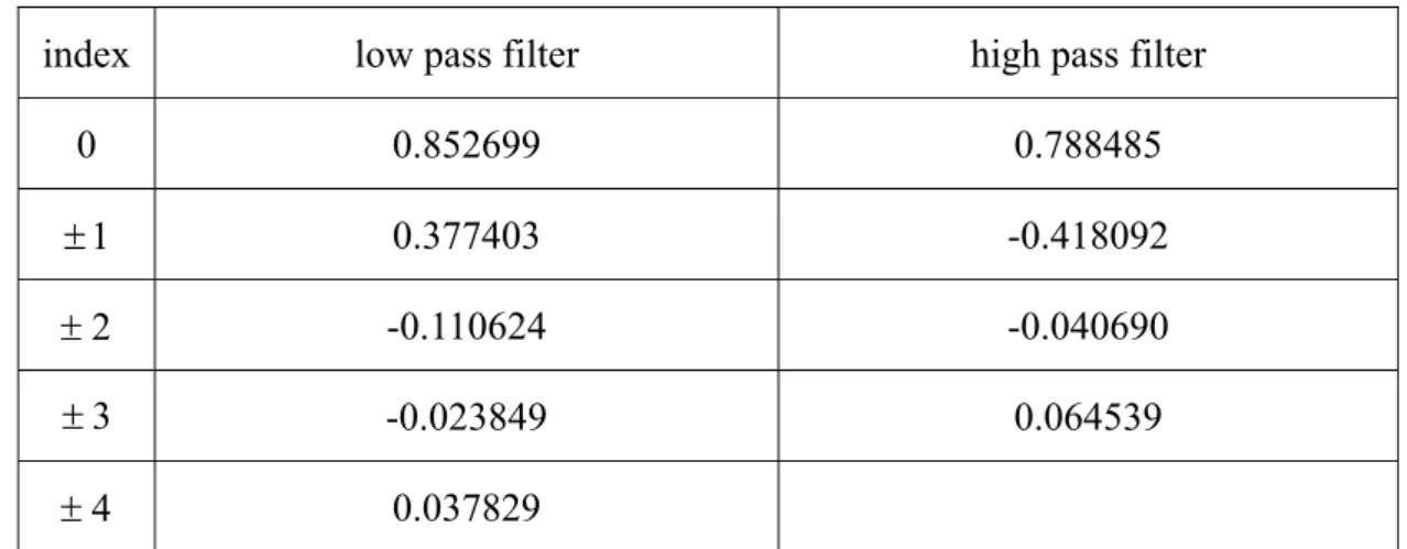
(31) n- d n ] where d m and d n are the closet integer to dm and dn. The temporal high-pass coefficients are calculated on the predicted frame by (1). The motion estimation would link every pixel in the predicted frame to another pixel in the reference frame; therefore, all pixels in the predicted frame are connected.. (. ). ~ H [m, n ] = B[m, n] − A[m − d m , n − d n ]. 2. (1). .. The temporal low-pass coefficients are generated on the reference frame and the pixels on the reference frame can be classified as connected and unconnected. The low-pass coefficients of the connected pixel are calculated by:. [. ]. [. ]. [. ~ L m − dm , n − dn = H m − dm + dm , n − dn + dn + 2A m − dm , n − dn. ].. (2). The low-pass coefficients of the unconnected pixels are calculated by:. L[m, n] = 2 A[m, n] .. (3). When decoding, A can be reconstructed by:. [. ] ([. ]. [. ~ A m − dm , n − dn = L m − dm , n − dn − H m − dm + dm , n − dn + dn. ]). 2. .. (4). After reconstruction of A, we can reconstruct B by: ~ B[m, n] = 2 H [m, n] + A[m − d m , n − d n ]. .. (5). In (4), we can see L and H are still necessary for the reconstruction of A , and. H only contains the information of interpolated pixels in A . But this interpolated information is also available in L . So it is canceled out in (4). Thus the interpolation algorithm has no influence on the perfect reconstruction [13].. 2.3.3 Spatial Analysis Spatial wavelet transform is performed on every residual frame after motion compensated temporal filtering. If the video sequence is composed of YUV component, then spatial wavelet transform is performed on all the three components. 18.

(32) The coefficients of the used filters are shown in Table 2-1. index. low pass filter. high pass filter. 0. 0.852699. 0.788485. ±1. 0.377403. -0.418092. ±2. -0.110624. -0.040690. ±3. -0.023849. 0.064539. ±4. 0.037829 Table 2-1 The coefficients of filters.. 2.3.4 Embedded ZeroBlock Coding After temporal and spatial decomposition, the coefficients are coded by “Embedded ZeroBlock Coding (EZBC)”. Because of the zeroblock coding and context modeling, this coding algorithm can achieve low computational complexity and high compression efficiency. The coding process begins with the creation of the quad-tree based set partitioning data representations on bit-planes for each individual subband. The bottom of the quad-tree level is the pixel level and consists of the magnitude of each subband coefficients. Each quad-tree node of the next higher level is then set to the maximum value of its four corresponding nodes at the current level, as illustrated in Figure 2-14(a). By recursively grouping the coefficients, the top quad-tree node would correspond to the maximum magnitude of all the coefficients from the same subband. Then the bitplanes of subband coefficients from the most significant bit toward the significant bit is progressively encoded. If a node is significant, it is split into four descendent nodes. This procedure is recursively down until the bottom level, as illustrated in Figure 2-14 (b). Once a pixel is significant, its sign bit is coded. Each bitplane coding pass is finished with a bitplane refinement subpass which further 19.

(33) refines the significant subband coefficients from the previous bitplane pass. So we can send data in the order of their importance in this way. 0: Significant node Significant node. Quad-tree Level 2. 1. 1: Insignificant node Codestream 1 1100 00010010. Quad-tree Level 1. 1. 1. 0. 0. Quad-tree Level 0 (Pixel level). 0. 0. 0. 0. 0. 1. 1. 0. 0. 0. 0. 0. 0. 0. 0. 0. (a) Quad-tree bulit up. (b) Quad-tree splitting. Figure 2-14 Quad-tree generation of the image [10].. 2.3.5 Entropy Coding This is the final process of encoding. At this time, the processed data contains motion information and the EZBC coded image data. Because HVSBM uses variable block size when doing motion estimation, the information of how the block sizes are arranged need to be coded. This information is contained in the quad-tree structure and coded in the map representation as shown in Figure 2-15. Then the map code is inserted in the encoded bit-stream.. 0: with child 1: no child MAP Code: 0, 0001, 0000. Figure 2-15 Map representation of the quad-tree. 20.

(34) The motion vectors of the leaf node blocks are sent into the adaptive arithmetic coder following the raster scan shown in Figure 2-16. The scanning order is the recursive raster scan of the leaf nodes in the motion vector quad-tree.. Figure 2-16 Motion vector coding scanning trail. The arithmetic coder initially sets the probability of all symbols to the same value. Then the symbol probability is updated after each symbol is encoded by accumulating the occurrence of the symbol during encoding. Combined with EZBC’s quad-tree representation of the image data, the strong statistical dependencies among bit-planes, resolution scale, and quad-tree levels are exploited [10].. 2.4 Scalable Video Coding Mass audiences have different viewing requirement and the bandwidth and capacity of each server on the network is different. So it is important to meet different requirement. The principle idea of the scalable video coding is that the encoded bitstream can be flexibly truncated to meet the requirements after the compressed bitstream has been generated. Digital video can have many specifications, such as picture size, picture quality, and picture playback rate. Because different user may have different requirement on these specifications, the ability to scale and choose different combinations of these 21.

(35) video specifications is crucial for simultaneous distribution to disparate clients .The main concept of the scalable video coding is “generate-once, scale-many”. Most people have more demand on the picture quality. There are three video scaling parameters that influence the viewing quality most: 1) the distortion of the picture, 2) the spatial resolution of the image, 3) the temporal resolution of the video. One major feature of the interframe wavelet coding is the ability to achieve all of the three mentioned video scalable features in one single coding algorithm. We will introduce these three scaling parameters in the following subsections.. 2.4.1 Rate/SNR Scalability The rate/SNR scalability is the ability that a single compressed bitstream can be decoded into different coding bit-rates/quality levels. The basic element of the interframe wavelet video coding encoded bitstream is GOP. It is composed by GOP header, the motion information, and the image data, as shown in Figure 2-17. The motion information is required to construct the motion fields that are used in the motion compensated temporal filtering so it is usually sent without any modifications. The image data is used to construct residual frames and it will be truncated to match the requested bit rate. GOP Header. Video Header. Motion Information Data. GOP. GOP. Residual Image Data. ……. GOP. Figure 2-17 The interframe wavelet video coding encoded bitstream. The rate/SNR scalability is achieved by truncation the image data to match the required bit rate. In the EZBC process, the bit-stream is arranged in an embedded structure such that information bits are saved in accordance to the importance of the data. During the process of the encoding of the EZBC, the information of how many 22.

(36) bits are used in the subband is marked as a parameter file, indicating the truncation points of the encoded residual image data in the video bit-stream. When doing truncating, the total bit rate of the GOP header, motion information, and the image data must equal to or less than the required bit rate. So the truncating process will find the corresponding truncation point and read the image data before the truncation point then package. Figure 2-18 shows the rate/SNR scalability.. 300kbps PSNR=32.2 dB. 500kbps PSNR=34.6 dB. GOP Header Motion Info.. 1000kbps PSNR=38.2 dB. Residual Image Data. Figure 2-18 Rate/SNR scalability.. 2.4.2 Spatial Scalability When performing spatial decomposition on the residual image, the image is down-sampled to lower resolutions. Therefore, the spatial scalability is inherent in the interframe wavelet video coder. However, the spatial scalability is not fine-tuned scalable. For an original frame size of m-by-n, the spatial scalability of the image is restricted to the size of m/2p-by-n/2p where p is an integer. The truncation process keeps the information of subbands that are lower than or equal to the required spatial resolution and truncates the other subbands. Upon decoding, the motion vectors of the motion information are scaled by the factor of p, regarding the rescaled size. The residual image data are then motion compensated temporal synthesized with the scaled set of motion vectors to reconstruct 23.

(37) the original sequence.. Figure 2-19 Spatial scalability.. 2.4.3 Temporal Scalability The interframe wavelet transform will create a temporal pyramid after MCTF. In order to reduce the amount of transform data, we can discard the temporal high-pass frame, as that shown in Figure 2-20(a). To achieve temporal scalability, the truncation process keeps the subset of images that are needed to generate the required level of temporal pyramid, as that shown in Figure 2-20(b).. 24.

(38) 30Hz Video Sequence 15Hz Video Sequence H. H. H. H. H. H. H. H1 7.5Hz Video Sequence. H2. H2. H2. H2 3.25Hz Video Sequence H3. H3. H4. L. (a) Temporal pyramid and temporal down-scaled sequence. GOP Header. L. H4. HH3. HHHH2. HHHHHHHH1. 7.5 Hz Video 15 Hz Video 30 Hz Video (b) The GOP of the temporal scaled sequence Figure 2-20 Temporal scalability. If motion estimated motion trajectory is not perfectly matched to the original video sequence, the temporal filtering process might generate some motion artifacts [14].. 25.

(39) Chapter 3 3D Subband Video Coding Using Barbell Lifting In 68th MPEG meeting (March, 2004, Munich), MSRA proposed its MCTF structure and 3D ESCOT entropy coder. The 3D ESCOT entropy coder performs almost as well as the 3D EBCOT that JPEG2000 used. Figure 3-1 shows the block diagram of this coding structure [15]. This proposed video coding algorithm has two different concepts. They are Barbell lifting and 3D ESCOT entropy coding. The motion estimation scheme of this video coding algorithm is not HVSBM but a motion estimation scheme used in H.264. We will describe them in the following subsections.. Figure 3-1 The block diagram of the 3D subband video coding using Barbell lifting [15].. 3.1 Barbell Lifting MSRA proposes this Barbell lifting algorithm for doing temporal decomposition [15]. Barbell lifting uses a set of pixels instead of a pixel as the input, as that shown in Figure 3-2. The Barbell lifting can provide perfect reconstruction, sub-sample decomposition but still with critically sampled transformed coefficients. 26.

(40) t. a. sˆ0. a. sˆ2. s1. sˆ2 = f2 (S2 ). sˆ0 = f0 (S0 ) S1. S0. S2. Figure 3-2 The Barbell lifting [15]. Assume that S0, S1, and S2 are three consecutive frames in a video sequence. Functions f 0 () and f 2 () are called as Barbell functions and they can be any linear or non-linear functions that take any pixels in the same frames as variables. The Barbell functions can also vary from pixel to pixel. Therefore the basic Barbell lifting step is formulated as: t = a × sˆ0 + s1 + a × sˆ2 ,. (6). where a is a filter parameter. The Barbell lifting includes two stages. They are prediction stage and update stage. The prediction stage is applied to the video sequence first. It takes the original input frames to generate the high-pass frames, as shown in Figure 3-3.. 27.

(41) x1 xˆ = f ( X ) 2 2 2. xˆ 0 = f 0 ( X 0 ). xˆ ' 2 = f ' 2 ( X 2 ). xˆ 4 = f 4 ( X 4 ). Figure 3-3 The prediction stage of the Barbell lifting. Then the update stage uses the available high-pass frames and the even frames to generate the low-pass frames, as shown in Figure 3-4.. hˆ0 = g 0 ( H 0 ). hˆ'1 = g '1 ( H 1 ). hˆ1 = g1 ( H 1 ). hˆ' 0 = g ' 0 ( H 0 ). Figure 3-4 The update stage of the Barbell lifting.. 3.1.1 The Prediction Stage ( x ± 1, y ± 1). ( x, y ). ( Δx , Δy ). ( Δx0 , Δy 0 ). ( Δxm , Δy n ). ( Δx , Δy ). ( x, y ). ( x, y ). ( Δx ±1 , Δy ±1 ). ( x, y ). ( Δx M , Δy N ). ( Δx 0 , Δy 0 ). Figure 3-5 The Barbell functions used in the prediction stage. 28.

(42) Figure 3-5 shows some examples of Barbell functions used in the prediction stage and Figure 3-5(a) is the integer motion alignment case and the Barbell function of this case is: f = Fi ( x + Δx, y + Δy ) ,. (7). where ( Δx, Δy ) is the motion vector of current pixel (x, y) and Fi is the previous frame. Figure 3-5(b) is the fractional-pixel motion alignment case and the Barbell function of this case is: f = ∑∑ α ( m, n ) Fi ( x + ⎣Δx ⎦ + m, y + ⎣Δy ⎦ + n ) , m. (8). n. where ⎣ ⎦ denotes the integer part of Δx and Δy . α ( m, n ) is the factor of the interpolation filter. Figure 3-5(c) is the multiple-to-one mapping case and the Barbell function of this case is: f = ∑∑ α ( m, n ) Fi ( x + Δx m , y + Δy n ) , m. (9). n. where α ( m, n ) is the weighting factor for each connected pixel. Figure 3-5(d) shows a special case that the current pixel (x, y) can use its motion vector ( Δx, Δy ) and the motion vectors of neighboring pixels to get multiple predictions from the previous frame and generate a new prediction. The Barbell function of this case is:. f =. ∑ ∑α (m, n) F ( x + Δx i. m. , y + Δy n ) ,. (10). m = 0, ±1 n = 0, ±1. where α ( m, n ) is the weighting factor.. 3.1.2 The Update Stage The prediction and update stages may has mismatch when pixels in different frames are aligned with motion vectors at fractional-pixel precision or without one-to-one 29.

(43) mapping. Generally speaking, the update and prediction stages use the same motion vector for saving overhead bits to code motion vectors, i.e., the motion vector of the update stage is the inverse one of the prediction stage. Figure 3-6 shows the mismatch problem.. (xm+1, yn+1) (xm+Δxm, yn+Δyn) (xm, yn). (xm+1, yn+1) (xm, yn) (xm-Δxm, yn-Δyn) (xm-1, yn-1). (xm-1, yn-1) (xm-2, yn-2). (xm-2, yn-2) Fi. Fj. Figure 3-6 The mismatch problem of motion in the prediction and update stages. As shown in Figure 3-6, the mismatch problem is that the prediction has the path from Fi ( xm , yn ) to Fj ( xm + Δxm , yn + Δyn ) but the update has the path from Fj ( xm , yn ) to Fi ( xm − Δxm , yn − Δyn ) . Barbell lifting can solve this mismatch problem. In the update stage, the obtained high-pass coefficients are likely distributed to those pixels that are used to calculate the high-pass coefficient in the prediction stage. Assuming that equation (9) is the. Barbell function used in the prediction stage now. We can calculate the high-pass coefficients by combining equations (6) and (9). Then we calculate the high-pass coefficients by: h j ( x, y ) = F j ( x, y ) + ∑∑∑ aiα i , j ( x, y, m, n ) Fi ( x + Δxm , y + Δy n ) , i. m. (11). n. where αi , j ( x, y , m, n ) is the Barbell parameter specified by the coordination x, y, m, n. Then we can calculate low-pass coefficients in the same way by: 30.

(44) li ( x, y ) = Fi ( x, y ) + ∑∑∑ b jα i , j ( x, y , m, n )h j ( x + Δxm , y + Δy n ) . j. m. (12). n. It means that the high-pass coefficient will be added back exactly to the pixels that are predicted. For the above example, the predicted weight from Fi ( x m −1 , y n −1 ) to F j ( x m , y n ) is non-zero. So in the proposed technique, the update weight from F j ( x m , y n ) to Fi ( x m −1 , y n −1 ) , which equals to the predict weight, is also not zero.. 3.2 Spatial Decomposition. Figure 3-7 The frame after 3 level spatial decomposition. After temporal decomposition, the spatial decomposition is applied to each created residual frame. The filter used here is the Daubechies 9/7 filter and the analysis filter coefficients are shown in Table 3-1 [35]. The coefficients of the Daubechies 9/7 synthesis filter are shown in Table 5-1 [35]. index. Analysis low pass filter. Analysis high pass filter. 0. 0.6029490182363579. 1.115087052456994. ±1. 0.2668641184428723. -0.5912717631142470. ±2. -0.07822326652898785. -0.05754352622849957. ±3. -0.01686411844287495. 0.09127176311424948. ±4. 0.02674875741080976 31.

(45) Table 3-1 The coefficients of the Daubechies 9/7 analysis filters. The spatial decomposition can also be done on the LH, HL, and HH subbands of the first level decomposition. Thus we can get the important information in those subbands and code them.. 3.3 Multi-Layer Motion Estimation and Coding The video coding algorithm proposed by MSRA dose not use HVSBM in motion estimation. It uses a motion estimation method adopted in H.264 but makes some changes to achieve motion information scalability.. Figure 3-8 Multi-layer motion estimation and coding. It uses multi-layer motion estimation and coding as shown in Figure 3-8. It generates an embedded bitstream for motion, which consists of one base layer and a few enhancement layers. A coarse motion field can be reconstructed from the base layer and can be successively refined by subsequent enhancement layers. The motion vectors of the base layer are large and coarse and may be used for low bit rates. The motion vectors of enhancement layer are small with details and often used for high bit rates.. 3.4 3D ESCOT After temporal and spatial decomposition, the generated coefficients will be coded with 3D Embedded Subband Coding with Optimal Truncation (3D ESCOT) [16]. The 32.

(46) 3D ESCOT is in principle very similar to EBCOT used in JPEG2000 [9], which deals with 2D image coding. We can call 3D ESCOT as 3D EBCOT because it is an extension of EBCOT used to do 3D dimensional signal coding. 3D ESCOT can offers high compression efficiency and other functionalities, such as error resilience and random access. 3D ESCOT takes advantages of the orientation-invariant property of wavelet subbands to reduce the number of context and codes each subband independently so each subband can be decoded independently. Because of this feature, 3D ESCOT can achieve flexible spatial/temporal scalability and R-D optimization can be done within subbands to improve compression efficiency. Each subband is divided into 3D coding blocks and these blocks are coded independently. For each coefficient x[i, j, k] at position [i, j, k], we assign it a binary-valued state variable σ[i, j, k], which indicates the significance of this coefficient. χ[i, j, k] is defined as the sign of the x[i, j, k]. It is 0 when the sample is positive and 1 when the sample is negative. σ[i, j, k] is initialized to 0 and toggled to 1 when the x[i, j, k]’s first non-zero bit-plane value is encoded. There are three coding operations and when they will be used depends on σ[i, j, k]. Zero coding (ZC) and sign coding (SC) will be used to code x[i, j, k] if σ[i, j, k] = 0 and magnitude refinement (MR) will be used if σ[i, j, k] = 1. We will introduce these three coding operations as follows.. 3.4.1 Zero Coding If a coefficient x[i, j, k] is not yet significant in the previous but-planes, i.e., σ[i, j, k] = 0, ZC is used to code the new information about whether it becomes significant or not in the current bit-planes. ZC uses significant information about x[i, j, k]’s immediate neighbors as the context to code the its own significant information. There 33.

(47) are four types of neighbors as shown in Figure 3-9. Current sample Horizontal Neighbor Vertical Neighbor Temporal Neighbor Diagonal Neighbor. Figure 3-9 Four types of coding neighbors for zero coding. 1. Immediate horizontal neighbors. The number of these neighbors is 2 and the number of significant ones is denoted by h, 0≦h≦2. 2. Immediate vertical neighbors. The number of these neighbors is 2 and the number of significant ones is denoted by v, 0≦v≦2. 3. Immediate temporal neighbors. The number of these neighbors is 2 and the number of significant ones is denoted by a, 0≦a≦2. 4. Immediate temporal neighbors. The number of these neighbors is 12 and the number of significant ones is denoted by d, 0≦d≦12. Table 3-2 shows the context assignment map of ZC. If the conditions of two or more rows are satisfied in the same time, the low-numbered context is selected. LLL and. h. 2 1. 1. 1 0 0 0. 0 0 0 0. LLH. v. x ≥1 0. 0 2 1 0. 0 0 0 0. sub-band. a. x x. ≥1 0 0 0 ≥1 0 0 0 0. d. x x. x. x x x x. 3 2 1 0. context 0 0. 1. 2 3 4 5. 6 7 8 9. LHH. h. 2 1. 1. 1. sub-band. v+a. x ≥3 ≥1 ≥1 0. d. x x. context 0 0. 1. 1 0. 0. 0. 0. 0. 0 ≥3 ≥1 ≥1 0. 0. ≥4 x. ≥4 x x. ≥4 x. ≥4 x. 1. 3. 6. 8. 2 34. 4 5. 7. 9.

(48) HHH. d. ≥6 ≥4 ≥4 ≥2 ≥2 ≥2 ≥0 ≥0 ≥0 ≥0. sub-band. h+v+a. x. context 0. ≥3 x. ≥4 ≥2 x. ≥4 ≥2 1. 0. 1. 3. 6. 9. 2. 4. 5. 7. 8. Table 3-2 Context assignment map for ZC.. 3.4.2 Sign Coding SC is called to code χ[i, j, k], which is the sign of coefficient x[i, j, k], if x[i, j, k] becomes significant in the current bit-plane. SC also utilizes high-order context-based arithmetic coding to compress the sign symbols. The context models of arithmetic coding are based on three quantities hs, vs and ts. They are defined as follows: hs=min{1, max{-1, σ[i-1,j,k] × (1-2χ[i-1,j,k])+ σ[i+1,j,k]×(1-2χ[i+1,j,k])}},. (13). vs=min{1, max{-1, σ[i,j-1,k] × (1-2χ[i,j-1,k])+ σ[i,j+1,k] × (1-2χ[i,j+1,k])}},. (14). ts=min{1, max{-1, σ[i,j,k-1] × (1-2χ[i,j,k-1])+ σ[i,j,k+1] × (1-2χ[i,j,k+1])}}.. (15). Table 3-3 shows the context assignment map and sign prediction map of SC. χˆ is the sign symbol prediction under the given context and the symbol sent to the arithmetic coder is χˆ ♁χ hs=-1. hs =0. vs. -1. -1. -1. 0. 0. 0. 1. 1. 1. ts. -1. 0. 1. -1. 0. 1. -1. 0. 1. χˆ. 0. 0. 0. 0. 0. 0. 0. 0. 0. context 0. 1. 2. 3. 4. 5. 6. 7. 8. vs. -1 -1. -1. 0. 0. 0. 1. 1. 1. ts. -1 0. 1. -1. 0. 1. -1. 0. 1. χˆ. 0. 0. 0. 0. 1. 1. 1. 1. context 9. 0. 10 11 12 13 12 11 10 9 35.

(49) hs =1. vs. -1. -1. -1. 0. 0. 0. 1. 1. 1. ts. -1. 0. 1. -1. 0. 1. -1. 0. 1. χˆ. 1. 1. 1. 1. 1. 1. 1. 1. 1. context 8. 7. 6. 5. 4. 3. 2. 1. 0. Table 3-3 Context assignment and sign prediction map for SC.. 3.4.3 Magnitude Refinement MR is called to code new information about x[i, j, k] if σ[i, j, k] was switched to 1 in the previous bit-plane, i.e., it becomes significant. It uses three contexts for arithmetic coding. 1. The context of x[i, j, k] is 0 if MR not yet used for x[i, j, k]. 2. The context of x[i, j, k] is 1 if MR has been used for x[i, j, k] and x[i, j, k] has at least one significant neighbor by now. 3. Otherwise, the context is 2.. 3.4.4 Fractional Bit-Plane Coding The practical coding gain of 3D ESCOT is higher than 3D SPIHT because SC and MR have high-order context modeling and the use of fractional bit-plane coding [16]. The fractional bit-plane coding can provides a practical means of scanning the wavelet coefficients within each bit-plane for rate-distortion (R-D) optimization at different rates. There are three different fractional bit-plane passes and the scanning order in each of them is along the i-direction firstly, then the j-direction and the k-direction lastly.. 3.4.4.1 Significance Propagation Pass If the coefficients which are not yet significant but have “preferred neighborhood” are processed by this pass. A coefficient has a “preferred neighborhood” if and only if 36.

(50) the coefficient has at least one significant immediate diagonal neighbor for HHH subband or horizontal, vertical, temporal neighbor for the other types of subband. For these coefficients, we apply the ZC to code their significance information in the current bit-plane of this coefficient. If the coefficient becomes significant in the current bit-plane, then SC is used to code the sign.. 3.4.4.2 Magnitude Refinement Pass If the coefficient became significant in the previous bit-plane, it will be coded in this pass. The binary bits corresponding to these coefficients in the current bit-plane are coded by MR.. 3.4.4.3 Normalization Pass It is used to code the coefficients if it was not coded in the previous two passes. Because these coefficients are not yet significant, they are only processed by ZC and SC.. 3.5 Bitstream Truncation and Scalability After 3D ESCOT on each subband, an embedded bitstream is generated for each subband. In order to satisfy the requested bit rate, bitstreams corresponding to different subbands will be truncated and multiplexed together to construct final bitstream then transmitted to the receiver. The rate control problem is how to truncate and multiplex bitstreams to create the final bitstream that achieves the best R-D optimization. The basic problem of rate control is that given a target bit rate R0, how to construct a bitstream that satisfies the bit rate constraint and minimizes the overall distortion. Shoman and Gersho proposed a Lagrange’s theorem that can solve this problem [17]. 37.

(51) Taubman extends this algorithm to the rate control of EBCOT [9]. EBCOT partitions the subbands representing the image into a collection of relatively small code-blocks, Bi, whose embedded bitstreams may be truncated to the B. rate Rin . The contribution from Bi to the distortion in the reconstructed image is B. denoted Din , for each truncation point n. Assuming that the distortion of each code-block is independent and additive. Thus the overall reconstructed image distortion D can be represented by: D = ∑ Dini ,. (16). i. where ni denotes the truncation point selected for code-block Bi. Din is calculated by: B. Din = wb2i. ∑ ( s [k ] − s. k∈Bi. i. n i. [k ]) 2 ,. (17). where si [k ] is the 2D sequence of subband coefficients in code-block Bi. sin [k ] is B. the quantized representation of these coefficients associated with truncation point n, and wbi is the L2-norm of the wavelet basis functions for the subband, bi, to which code-block Bi belongs. B. R-D optimization algorithm should select truncation points ni for each code-block Bi such that the sum of Rini or Dini meets the constraint imposed by Rmax or Dmax B. and also the sum of Dini or Rini is the minimum value. They are described as follows:. ∑D. = D = Dmin , given. ∑R. = R = Rmin , given. ni i. i. ∑R. = R ≤ Rmax ,. (18). ∑D. = D ≤ Dmax .. (19). ni i. i. or ni i. i. ni i. i. Recently, several R-D optimization algorithms have been proposed to solve this 38.

(52) problem [18]. It is noticeable that all these algorithms are applicable to convex curves. Convex curves are the curves that the slopes are strictly decreasing. Some R-D optimization algorithms are based on Lagrange’s theorem, such as the Lagrange multiplier used in EBCOT [9]. Lagrange’s theorem states that the sum of continuous functions with boundary condition is optimized at the points with equal slopes as shown below: ( D(λ ) + λR (λ )) = ∑ ( Dini + λRini ) . λ. λ. (20). i. Any set of truncation points, { niλ }, which minimizes ( D(λ ) + λR(λ )) for some λ is optimal in the sense that the distortion cannot be reduced without increasing the overall rate or vice-versa. If we can find a value of λ such that the truncation points minimize ( D(λ ) + λR(λ )) yields R (λ ) = Rmax , then this set of truncation points must be an optimal solution to the R-D algorithm based on Lagrange’s theorem. Because the number of truncation points in a code-block is finite, we can not find the value of λ such that R(λ ) exactly equals to Rmax . However, since the code-block in EBCOT is very small such that the total number of truncation points is very large, we can find the smallest value of λ such that R (λ ) ≤ Rmax . In order to find the optimal truncation point sets niλ for any given λ , we need to know the rate-distortion (R-D) pair of each truncation points. λ can be viewed as the R-D slope of the optimal truncation point sets. We can find the R-D slope of each truncation point by calculating the bitstrean length and distortion at that point. Thus we can construct an operational R-D curve for each code-block. 1) Assume n is the number of the truncation points, and 0≦j≦n. 2) For j = 0, 1, 2, …, n, 0 is the beginning of the code-block, not a truncation point. ΔDi j Di j −1 − Di j = j , where Ri j is the The R-D slope of each truncation point j is j j −1 ΔRi Ri − Ri 39.

(53) accumulative bit length of truncation point j in code block i and Di j is the accumulative distortion of truncation point j in code block i. Generally. speaking,. Ri j ≥ Ri j −1 ≥ Ri j − 2 ≥ ... ≥ Ri0 = 0. and. Di j ≤ Di j −1 ≤ Di j − 2 ≤ ... ≤ Di0 = the distortion when the coefficients of the code-block. are all 0. We just need to package the truncation points with the R-D slope bigger than or equal to λ , then we can achieve the optimal R-D. In 3D ESCOT, the end of each fractional bit-plane is a candidate truncation point. The R-D slope of each truncation points can be obtained by calculating the bitstrean length and distortion [16]. Then we can construct an operational R-D curve for each subband and find its convex hull. All valid truncation points must lie on this convex hull such that the R-D optimality at each truncation point can be guaranteed. If the truncation point does not have a strictly decreasing R-D slope (i.e., it has larger distortion than the previous truncation point), it will be discarded. In order to find the best threshold value λ , we first set an arbitrary value of λ . If the R-D slope of this truncation point is bigger than or equal to λ , this truncation point will be packaged. After we process all of the truncation points, we obtain the final bitstream. If the bit rate of this bit-stream is larger than that of requested, the value of λ will be set larger to find the final bitstream again. Otherwise, the value of λ will be set smaller. We use this method recursively to find the final bitstream that has bit rate smaller than or equal to the requested bit rate.. 40.

(54) Chapter 4 Human Visual System 4.1 Human Vision. Figure 4-1 Cross-section of human eye [19]. Figure 4-1 shows the cross-section of a human eye [19]. Through the optics of the eye, the visual input is projected onto the retina, the neural tissue at the back of eye composed of the photoreceptor mosaic [20]. The photoreceptors sample the image and convert the input image to the signals that can be interpreted by the visual cortex of the brain. Photoreceptors have Rhodopsin which is very sensitivity to light. When Rhodopsin receives the energy of light, it will decompose into Vitamins A, Protein, and impulse signal. The impulse signal will be processed by the Bipolar cell and Ganglion cell then passed through optical nerves into the brain as shown in Figure 4-2 [21]. The Vitamins A, Protein, and Nutrition will be combined together and converted 41.

(55) to Rhodopsin by the effect of Enzyme. Then the Rhodopsin can be used again.. Figure 4-2 The process of the visual input signal [21]. There two types of photoreceptors, rods and cones. Rods are relatively long and thin. They are used to view at lower several orders of magnitude of illumination, i.e., under scotopic conditions. Cones are relatively shorter and thicker and they are less sensitive than rods. They are used to view at the higher 5 to 6 orders of magnitude of illumination, i.e., under photopic conditions. The cones are concentrated in the fovea, the region of highest visual acuity, which covers approximately two degrees of visual angle on the retina. The cones are also responsible for color vision. There three types of cones. They are L-cones, M-cones, and S-cones. L-cones are also called Red cones and they are sensitive to long wavelengths. M-cones are also called Green cones and they are sensitive to medium wavelengths. S-cones are also called Blue cones and they are sensitive to short wavelengths. Figure 4-3 shows the relative sensitivity of each photoreceptor [21].. 42.

(56) Figure 4-3 Relative sensitivity of each photoreceptor [21].. 4.2 Color Representation Colors do not exist in natural world. To human perception, colors are related to the wavelength of light. As describes above, the retina of human eye contains 3 different color receptors: red, green, and blue. The different cones have different sensitivity curve to light of different frequency. Thus, the combination of different sensitivity curve to light can produce different color recognition. Due to this structure of human eye, any color appeared to human eye can be specified by a weighted combination of three so-called primary colors RGB. For the purpose of standardization, the CIE (Commission. Internationale. de. L'eclairage─. International. Commission. on. Illumination) chooses the following specific wavelength values to the three primary colors: blue (B) = 435.8nm, green (G) = 546.1nm, and red (R) = 700.0nm. Trichromatic theory says that any color S can be represented as a combination of 43.

(57) these 3 primaries R, G, and B. S = Rs·R + Gs·G + Bs·B. B. (21). Any 3 independent colors can be selected as primaries as long as one is not a mix of the other two. Different sets of primaries are related by linear transformations. There several color models, such as CIE RGB, CIE XYZ, CIE YUV, and CIE L*a*b*. We introduce CIE RGB and CIE XYZ here. 1. CIE RGB: 1) R, G, B = three spectral primary source. 2) Reference white: R = G = B = 1. 3) There exist negative tristimulus values. 4) The color is fully dependent on the wavelength. The three fixed RGB components acting alone cannot generate all spectrum colors (pure colors). This is an unresolved defect for color representation. 2. CIE XYZ 1) All color matching functions are positive. 2) Y = luminance 3) Reference white: X = Y = Z = 1. 4) This model is modified from RGB model such that all spectral tristimulus values are positive. Generally Speaking, Each color space can transform to another space. Equation (22) is the transformation from CIE RGB to CIE XYZ and equation (23) is CIE XYZ to CIE RGB. ⎡ X ⎤ ⎡ 2.365 − 0.515 0.005 ⎤ ⎡ R ⎤ ⎢ Y ⎥ = ⎢− 0.897 1.426 − 0.014⎥ ⎢G ⎥ . ⎢ ⎥ ⎢ ⎥⎢ ⎥ ⎢⎣ Z ⎥⎦ ⎢⎣ − 0.468 0.089 1.009 ⎥⎦ ⎢⎣ B ⎥⎦. 44. (22).