以人工類神經網路連結揚聲器客觀量測指標與主觀聽覺屬性之間的相關性

國

國

國

國

立

立

立

立

交

交

交

交

通

通

通

通

大

大

大

大

學

學

學

學

機械工程學系

碩 士 論 文

以人工類神經網路連結揚聲器客觀量測指標與

主觀聽覺屬性之間的相關性

Correlation of Objective Nonlinear Measures and

Subjective Timbral Attributes of Loudspeakers using

Artificial Neural

指導教授：白明憲

研 究 生：廖國志

以人工類神經網路連結揚聲器客觀量測指標與

主觀聽覺屬性之間的相關性

Correlation of Objective Nonlinear Measures and Subjective Timbral Attributes of Loudspeakers using Artificial Neural

研 研 研

研 究 究究究 生生生生：： ：： 廖國志廖國志廖國志 Student：廖國志 ：：：Chun-Jen Wang 指導教授

指導教授 指導教授

指導教授：：： ： 白明憲白明憲白明憲 白明憲 Advisor：：：Mingsian R.Bai ： 國立交通大學

機械工程學系 碩 士 論 文

A Thesis

Submitted to Department of Mechanical Engineering College of Engineering

National Chiao Tung University In Partial Fulfillment of Requirements

For the Degree of Master of Science

In

Mechanical Engineering June 2010

HsinChu, Taiwan, Republic of China.

中華民國九十

中華民國九十

中華民國九十

以人工類神經網路連結揚聲器客觀量測指標與

主觀聽覺屬性之間的相關性

研究生：廖國志

指導教授：白明憲 教授

國立交通大學 機械工程學系 碩士班

摘要

摘要

摘要

摘要

揚聲器在大訊號的情形下工作時，許多揚聲器的非線性效應便會

顯現，造成聲音的失真進而破壞音質。本研究的目的主要是連結動圈

式揚聲器客觀量測指標與主觀聽覺屬性之間的相關性。利用大訊號揚

聲器模型製造出數個非線性模型，並分別對非線性模型做客觀指標量

測以及主觀聽覺測試。再使用迴歸分析、多變異數分析來分析數據，

並使用 Fisher's LSD 檢測主觀聽覺測試結果是否在統計上有顯著的差

異。再來我們使用類神經網路來連結客觀量測指標與主觀聽覺屬性之

間的相關性。類神經網路對於非線性失真所造成的音質檢測，提供了

一個不需要做主觀聽覺測試，而且更有效率的方法。

Correlation of Objective Nonlinear Measures and Subjective Timbral Attributes of Loudspeakers using Artificial Neural

Student: Guo-Zhi Liao Advisor：Dr. Mingsian R.Bai

Department of Mechanical Engineering National Chiao-Tung University

Abstract

As a loudspeaker operates in the large-signal domain, nonlinear distortion may arise and impair the sound quality. This work aims to correlate various subjective audio attributes and the objective nonlinear measurements for moving-coil loudspeakers. Several nonlinear models of loudspeaker are created, based on a large-signal loudspeaker model. The data of subjective listening test were processed by the regression analysis, the multivariate analysis of variance (MANOVA), and the least significant difference method (Fisher’s LSD) as a post hoc test to justify the statistical significance of the results. The objective and subjective indices are correlated with the aid of an artificial neural network (ANN). The network proved effective in assessing subjectively the sound quality impairment due to nonlinear distortions of loudspeakers based on only objective measurements, without having to conduct listening tests.

誌謝

誌謝

誌謝

誌謝

短短兩年的研究生生涯轉眼即逝。在此感謝白明憲教授的諄諄教誨與照顧， 在白明憲教授的指導期間，深刻的感受到教授對於追求學問的熱忱，更是佩服教 授淵博的學問與解決問題的方法。在教授豐富的專業知識以及嚴謹的治學態度 下，使我能夠順利完成學業與論文，在此致上最誠摯的謝意。 在論文寫作方面，感謝本系呂宗熙教授和陳宗麟教授在百忙中撥冗閱讀，並 提出寶貴的意見與指導，使得本文的內容更趨完善與充實，在此學生致上無限的 感激。 在這兩年的研究生生涯中，承蒙博士班林家鴻學長、李雨容學姊、陳勁誠學 長、劉志傑學長，以及已畢業的王俊仁學長、郭育志學長、何克男學長、艾學安 學長、劉冠良學長在研究與學業上的適時指點，並有幸與廖士涵同學、陳俊宏同 學、張濬閣同學、桂振益同學、曾智文同學、劉孆婷同學互相切磋討論，讓我獲 益甚多。此外學弟王俊凱、吳俊慶、許書豪、衛帝安、馬瑞彬在生活上的朝夕相 處與砥礪磨練，亦值得細細回憶。因為有了你們，讓實驗室裡總是充滿歡笑。能 順利取得碩士學位，要感謝的人很多，上述名單恐有疏漏，在此一併致上我最深 的謝意。 最後僅以此篇論文，獻給我摯愛的家人，父親廖世涼先生、母親程月招女士、 大妹廖怡婷以及小妹廖怡茹，這一路上，因為有你們的付出與支持，給了我最大 的精神支柱，也讓我有勇氣面對更艱難的挑戰。

TABLE OF CONTENTS

摘要 摘要 摘要 摘要... i Abstract ... ii 誌謝 誌謝 誌謝 誌謝... iii TABLE OF CONTENTS ... iv LIST OF TABLES ... v LIST OF FIGURES ... vi 1. INTRODUCTION... 1

2. THE LARGE-SIGNAL MODEL OF MOVING-COIL LOUDSPEAKERS .. 3

2.1 Nonlinearities of Moving-Coil Loudspeakers ... 3

2.2 Large-Signal Model ... 4

3. OBJECTIVE EVALUATION BY NUMERICAL SIMULATION ... 5

3.1 Measures of Nonlinear of Symptoms ... 5

3.2 Relations between Nonlinear Causes and Symptoms of Loudspeakers .... 6

4. SUBJECTIVE LISTENING TESTS ... 7

4.1 Experimental Arrangement ... 7

4.2 Results of the Listening Test ... 9

5. ARTIFICIAL NEURAL NETWORKS ... 10

6. CONCLUSIONS ... 13

7. APPENDIX ... 14

Design of a MEMS microphone using SA method ... 14

7.1. Quasi-Static model ... 14

7.2 Linear Dynamic Model ... 16

7.3 SA method ... 18

LIST OF TABLES

Table 1. The relations between nonlinear causes and symptoms of moving-coil

loudspeakers. ... 25 Table 2. The MANOVA output of the listening test for the fifteen nonlinear

loudspeaker models. Cases with significance value p below 0.05 indicate that statistically significant difference exists among all cases. ... 26 Table 3. Multiple regression of Total Preference in relation to Fidelity, Fullness and

Artifacts... 27 Table 4. Multiple regression analysis of Total Preference in relation to HD₂, HD₃,

2

IMD and IMD₃. ... 28 Table 5. Fifteen nonlinear models with variations on speaker parameters of

loudspeaker A. The first ten cases of objective index were selected as the input for training the ANN. ... 29 Table 6. The target output (listening test result) of the ANN. The first ten cases of

objective index were selected as the target output data for training the ANN. The grading scale ranges from 1 to 5. ... 30 Table 7. Four nonlinear distortions, HD₂, HD₃, IMD₂ and IMD₃, of the

LIST OF FIGURES

Fig. 1 Electroacoustic analogous circuit of a moving-coil loudspeaker. (a) The equivalent circuit. (b) The circuit of the thermal model. ... 32 Fig. 2 The flowchart of the modeling and verification procedure for the

ANN-based loudspeaker assessment system ... 33 Fig. 3 The result of the listening test for the fifteen nonlinear loudspeaker models.

The means and spreads (with 95% confidence intervals) of the grades are indicated in the figure. The x-axis and y-axis correspond to the nonlinear models and the grades, respectively. ... 34 Fig. 4 The schematic of the neuron. The symbol a_n is the input, w_n is the

weight, b is the bias, and o is output. ... 35

Fig. 5 The structure of the back-propagation ANN. The symbol a is the hidden layer, a hidden layer of fifteen neurons, xi _{is the input layer of the}

nonlinear distortion measures HD HD IMD2, 3, 2 _and IMD3_, wij _and wk

are the weights, b1 _and b2 _{are the bias units, and} y _{is the output of the}

subjective attributes: Fidelity, Fullness, Artifacts and Total Preference. ... 36 Fig. 6 Comparison of Total preference, Fidelity, Fullness and Artifacts predicted by the ANN and the subjective data obtained from the listening test for the last five cases (in-group verification).

5

Output Target

Error= − ... 37 Fig. 7 The out-group test result of the listening test for the four nonlinear

loudspeaker models. The means and spreads (with 95% confidence intervals) of the grades are indicated in the figure. The x-axis and y-axis correspond to the nonlinear models and the grades, respectively. ... 38 Fig. 8 The results of the out-group test of the ANN based on the Loudspeaker

model B. Total preference, Fidelity, Fullness and Artifacts predicted by the ANN and the subjective data obtained from the listening test are

compared.

5

Output Target

Error= − ... 39 Fig. 9 The flow chart of the iterative procedure from FDM method for the coupled

equation system ... 40 Fig. 10 Acoustical system includes the sound radiation, air gap, back chamber and

acoustical holes influence. ... 41 Fig. 11 Combination of mechanical and electrical system. ... 41

Fig. 12 The comprehensive system combines the acoustical, mechanical and electrical system. ... 42

1. INTRODUCTION

Loudspeaker evaluation has been a long-standing issue in that it involves not only physical aspects but also psychoacoustic features which are largely subjective. More often than not, audiophiles trust more on the experience of human experts than the frequency response on the data sheet. This is why sometimes it is regarded as art rather than science to assess loudspeaker quality and the price at the marketplace can vary drastically without bound. Many factors can contribute to the overall sound quality of a loudspeaker. Among these factors, nonlinear distortions have profound impact on the timbral quality of a mono-channel loudspeaker. To address the issue, this paper aims at exploring the correlation between the objective measures of nonlinear distortions and the subjective perception of timbral quality associated with these distortions. If this correlation can be found, akin to the PEAQ[1] for audio codec assessment, then it is possible to develop an automatic system for loudspeaker evaluation, without having to conduct human listening tests.

Loudspeakers can be evaluated with objective measurements and subjective listening tests. The latter are generally time consuming and tedious to carry out. Lavandier et al. investigated subjective dimensions based on underlying perceived differences between loudspeakers [2]. Multidimensional scaling technique was employed to analyze temporal and spectral data of listening tests. Two principal perceptual dimensions, the bass/treble balance and the medium emergence, were identified for loudspeaker evaluation. Liu et al. [3]-[4] attempted to evaluate loudspeakers using sound quality metrics [5] suggested by Zwicker and Fastl. Metrics including loudness, sharpness, fluctuation strength and roughness that are widely used in assessing “noise” quality of products are employed for quantifying the timbral quality of loudspeakers. Listening tests were conducted in that study.

subjective attributes with special regards to nonlinear distortion of moving-coil loudspeakers. Traditionally, many objective indices such as sensitivity, efficiency, directivity pattern, nonlinear distortions, etc., can be used for loudspeaker evaluation. Among these indices, nonlinear distortions have direct impact on the perception of timbral quality produced by loudspeakers. As loudspeakers operate in the large-signal regime, nonlinear distortions may arise and can strongly impair sound quality. Metrics such as DC-displacement, harmonic distortion, inter-modulation, etc., can be used to quantify loudspeaker nonlinearities [6]-[7]. In this paper, four types of nonlinear metrics, HD2,HD3,IMD2, and IMD3 are used in the objective

measurements. Nonlinear distortions of a loudspeaker may arise as a result of various causes such as nonlinear compliance, nonlinear force factor, nonlinear inductance, etc [8]-[9]. In order to produce a sufficient database of nonlinear distortion, a large-signal model [10]-[13] is employed in this study to simulate large-signal responses of loudspeakers.

With the database, an artificial neural network (ANN) [14]-[15] was trained to correlate the objective nonlinear indices and the subjective attributes obtained in listening tests. Two loudspeaker models A and B were used in this study for in-group and out-group verifications, respectively. An ANN was established on the basis of fifteen nonlinear models of loudspeaker A and the human perceptions of nonlinear distortions in listening tests. Fifteen nonlinear models of loudspeaker A were then used for in-group verification. Among the models, ten nonlinear models are used to train the neural network, and the remainder is used to verify the ANN. For out-group verification, four nonlinear models derived from loudspeaker B were used. The assessment predicted by the ANN was compared to a listening test conducted for the loudspeaker B. With robustness so justified, the network serves for an automatic loudspeaker evaluation system, without resorting to listening tests.

2. THE LARGE-SIGNAL MODEL OF MOVING-COIL LOUDSPEAKERS

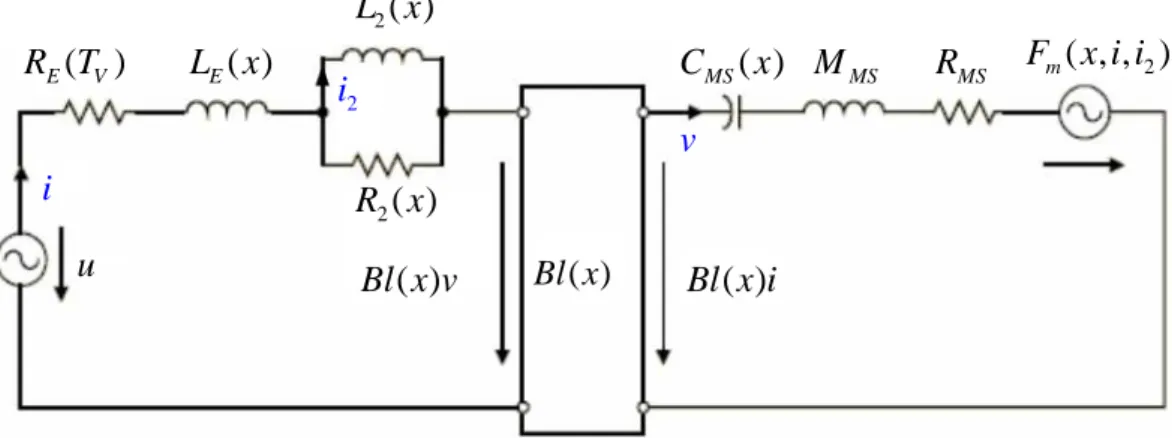
Sufficient amount of training data are required to establish a reliable ANN. Instead of gathering data from a large number of real loudspeakers, we opt for a more practical approach by using a large-signal moving-coil loudspeaker model, as described in this section. At low frequencies where the wavelength is large in comparison to the geometric dimensions, the state of a loudspeaker can be described by a lumped parameter model. In Fig. 1(a), the model is shown in terms of electroacoustic equivalent circuits coupled in the electrical, mechanical and acoustical domains [10]-[12]. The lumped parameters in the circuits such as the force factorBl x( ), the mechanical compliance C_MS( )x and the voice coil inductance

( )

E

L x can vary with the displacement of the voice coil.

2.1 Nonlinearities of Moving-Coil Loudspeakers

Four types of nonlinearity of moving-coil loudspeakers employed in the

large-signal model are summarized as follows:

1. Loudspeaker stiffness KMS( )x : the mechanical stiffness of driver suspension

which is also defined as the inverse of mechanical compliance C_MS( )x . The restoring

force F =KMS( )x x of the suspension system can cause nonlinear distortions.

2. Force factor Bl x :( ) instantaneous electrodynamic coupling factor between the

mechanical and electrical domains, where B is flux density and l is the effective

length of the voice coil. The force factor Bl x( ) is not a constant and is a function

of diaphragm displacement x. Two nonlinear effects force factor Bl x( ) can arise via: (a) back electromotive force (back-EMF) e=Bl x u( ) , where u is cone velocity, and (b) Lorentz force F =Bl x i( ) , where i is current.

3. Voice-coil inductance L x_E( ): the effective inductance of voice coil. L x_E( ) is

2.2 Large-Signal Model

A large-signal model is exploited to simulate nonlinear responses of loudspeaker in the large-signal regime. The loudspeaker model is represented using the equivalent circuit with nonlinear parameters, as shown in Fig. 1(a). The temperature increase in the voice coil is described by a separate thermal model shown in Fig. 1(b) [11]. The DC resistance R_E is dependent of the ambient temperature

A

T and the temperature increase of voice coil ∆TV.

( ) ( )(1 )

E A V E A V

R T + ∆T =R T + ∆δ T , (1)

where δ = 0.00393 degK-1 for copper and δ = 0.00393 degK-1 for aluminum. All parameters can be identified by a distortion analyzer [16]. The dynamics of the system depicted by Fig. 1(a) are governed by the following simultaneous ordinary differential equation system:

(

( )

)

(

2( )2

)

( ) E ( ) E V d L x i d L x i u iR T Bl x v dt dt = + + + , (2)

(

2 2

)

2 2 ( ) ( ) ( ) d L x i i i R x dt = − , (3) 2 2 2 ( ) m( , , ) MS MS MS d x dx Bl x i F x i i M R K x dt dt − = + + , (4) Choosing y1 =x, y2 =v, y3 =i and y4 =i2 as the state variables enables us to

rewrite Eqs. (2)-(4) into the following state-space equation:

2 3 4 1 1 2 3 2 2 3 4 2 2 2 2 2 2 0 1 0 0 1 ( ) 1 ( ) ( ) 1 _{2 2} ( ) ( ) ( ) ( ( ) ( )) ( ) 0 ( ) ( ) ( ) ( ) ( ) ( ) 0 0 ( ) ( ) E MS MS MS MS MS MS E E V E E E dL x dL x Bl x y y R _{dx dx} y _{M C x M M M} y y _{dL x} Bl x y R T R x R x y dx L x L x L x y dL x R x y R x _dx L x L x      ₊  − −            ₌ _{− −}  − +           _{ }  _{− −}        & & & & 2 3 4 0 0 1 ( ) 0 E y u y L x y            _{+ }           _ _ (5) The Runge-Kutta [17] numerical integration algorithm can readily be applied to solve

the state-apace equation for the nonlinear responses. Now that the velocity y2 =v

is obtained, the time-domain farfield sound pressure response can be calculated using a baffled point source model

0 ( , ) 2 D S dv p t r r dt ρ π = , (6)

where r is the distance between the diaphragm and the listening position, ρ₀ is the density of air and S is the area of the diaphragm. Note that pressure calculation D

of Eq. (6) requires numerical differentiation.

3. OBJECTIVE EVALUATION BY NUMERICAL SIMULATION

For the objective and subjective evaluations to be conducted next, nonlinearly

distorted signals were generated by the preceding large-signal model and reproduced

by a high-quality linear loudspeaker (iPod HiFi A1121).

3.1 Measures of Nonlinear of Symptoms

Various objective measures are adopted in the study to characterize loudspeaker

nonlinearity. The first basic measure is harmonic distortion (HD) that employs a

single-tone stimulus according to IEC standard 60268-5 [18]. The nth harmonic

distortion associated with f is defined as ₁

1 ( ) 100% n t P nf HD P = × , (7)

where P nf is the complex spectrum of sound pressure ( 1) P at the nth harmonic,

and P is the rms-value of the total signal within the averaging duration T _t

2 0 1 ( ) T t P p t dt T =

_∫

. (8)

Another important nonlinear measure is the Inter-modulation Distortion (IMD).

In this measure, two separate tones are used as stimuli, the first tone f is set to be ₁

higher than 8.5 f1. Furthermore, the amplitude U1 of the input voltage of the first

tone should be 4 times larger than the amplitude U₂ of the second tone. In the IMD test, the following two-tone excitation signal is used

1 1 2 2

( ) sin(2 ) sin(2 )

u t =U πf +U π f . (9) IMD accounts for extra frequency components due to intermodulations occurring at

2 1( 1, 2 )

f ±nf n= ⋅⋅⋅ . The nth-order IMD is defined as

2 1 2 1 2 ( ( 1) ) ( ( 1) ) 100% ( ) n P f n f P f n f IMD P f − − + + − = × . (10)

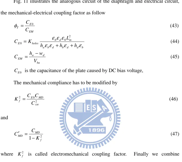
3.2 Relations between Nonlinear Causes and Symptoms of Loudspeakers

A rule-based logic is established according to the relations between the

nonlinear causes and symptoms of loudspeaker nonlinearities, as summarized in

Table1. Nonlinear distortions with various types and levels can be synthesized by

varying loudspeaker parameters,Bl x C( ), _MS( ), and x L x , which will be used in the _E( )

subsequent objective and subjective experiments.

The nonlinear causes in a loudspeaker’s response are subdivided into the

following two categories: critical nonlinearity variation and asymmetric nonlinearity

[6]-[7]:

1. Critical nonlinearity variation: “coil height” and “symmetrical limiting of

suspension” A symmetric curve usually produces the 3rd- and other odd-order

distortion components. To simulate the “coil height” and the “suspension limiting”

defect, the 2nd-degree term of the Bl - and the C_MS-series are usually multiplied by a

factor β >1 to increase their variations.

2 0 1 2 3 ( ) n i i i Bl x b b x βb x b x = ′ = + + +

∑

, (11) 2 0 1 2 3 ( ) n i MS i i C x c c x βc x c x = ′ = + + +

∑

(12)

2. Asymmetric nonlinearity: “coil offset,” and “asymmetry in CMS(x) and LE(x)”

Asymmetric Bl x( ) and C_MS( )x curves generally result in the 2nd- and other even-order distortion components. These defects can be modeled by shifting the

( )

Bl x and C_MS( )x curves on the x-axis by a small constantε.

0 ( ) ( ) ( ) n i i i Bl x Bl x ε b x ε = ′ = − =

∑

− (13) 0 ( ) ( ) ( ) n i MS MS i i C x C x ε c x ε = ′ = − =

∑

− . (14)

The inductance L x without shorting ring also exhibits asymmetric E( )

characteristics. To model this, we multiply the linear term of the L -series by a _E

factor β >1 to yield 0 1 2 ( ) n i E i i L x l βl x l x = ′ = + +

∑

(15)

4. SUBJECTIVE LISTENING TESTS

Figure 2illustrates the overall architecture of the experimental procedure. The

real time signal was used as the input for both in-group and out-group verifications.

Fifteen nonlinear models of loudspeaker A were created using the preceding large

signal model. These models will be used in the following objective and subjective

tests, separately. The objective nonlinear measures and subjective timbral attributes

obtained from these models serve as the input and the output to the ANN in the

training phase. After the ANN is trained, another four nonlinear models of

loudspeaker B were used for out-group verification in which the output of the ANN

and the listening test results will be compared.

4.1 Experimental Arrangement

Initially, subjective tests are conducted to obtain the relations between the

objective measures and the subjective attributes. There are fifteen experienced

test. Fifteen participants in the listening tests were instructed with definitions of the subjective attributes and procedures before the test began. The participants were asked to respond in a questionnaire after listening. The listening tests were carried out in a standard listening room (ITU-R BS. 1116-1 [19] ). The listeners sat 1m away from the monophonic loudspeaker (iPod HiFi A1121). The listening test complies with the MUSHRA procedure (ITU-R BS. 1534-1 [20] ), a modified double-blind Multi-Stimulus test with a hidden reference and a hidden anchor. The grading scale ranges from 1 to 5, indicating bad, poor, fair, good and excellent, respectively. Nonlinear loudspeaker models were created using the large-signal model with reference to the nonlinear cause-symptom logic summarized in Table 1. Fifteen nonlinear models of loudspeaker A, alongside the reference and anchor signals were created for the in-group listening tests. The test stimulus is a music clip of ”Hotel California.” The linear speaker model was used as the reference (the grading scale of the attributes is 5). The hidden anchor is a high-pass filtered input signal. The subjective attributes employed in this subjective test are the following four indices:

(1) Fidelity: clarity of the voice and the music. (2) Fullness: quality of low-frequency sound.

(3) Artifacts: any extraneous disturbances to the signal are considered as artifact.

(4) Total Preference: global attribute for listeners to judge the sound based on their own likes or dislikes.

Every subject is asked to grade the attributes above in sequence with the index Total Preference being the last item. It took approximately thirty minutes to finish a listening experiment.

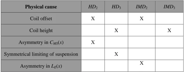
4.2 Results of the Listening Test

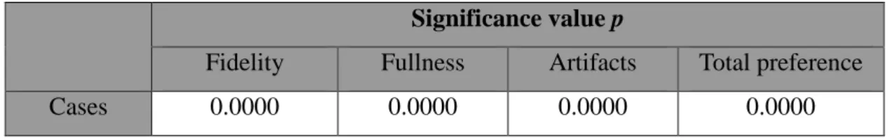
A listening test was conducted using the preceding subjective attributes. The cases with significance levels (p-values) of the test results processed using Multivariate ANalysis Of VAriance method (MANOVA) are shown in Table 2 and Fig. 3. The nonlinear models of loudspeaker A with p-values below 0.05 indicate that statistically significant difference exists among methods. The p-values of the attributes, Fidelity, Fullness, Artifacts and Total Preference are all zeros. Since significant difference is present in all attributes, we conduct a post hoc Fisher’s LSD test as multiple paired comparisons. There is neither statistically significant difference among Cases 3, 6, 10, 11 and 14, nor among Cases 9, 12 and 15. Apart from these cases, the results of the post hoc test indicate significant difference in pairs.

It can be observed in Fig 3 that Cases 4 and 7 received highest grades because of its lowHD₂, HD₃, IMD₂ andIMD₃ values.(<10%) Cases 6, 10, 11 and 14 received relatively higher grade due to its lower HD2 andHD3 values. Conversely,

Cases 9, 12 and 15 received the lowest grades due to its higher HD₂ andHD₃

values.

Figure 3 and Table 2 summarizes the influence of nonlinear distortions on the subjects. In this experiment, the nonlinear speaker models seem to result in marked difference (p < 0.05) in all subjective indices.

In order to examine how Total Preference is subjectively related to Fidelity, Fullness and Artifacts, multiple regression analysis was conducted for the listening test results, as shown in Table 3. The linear equation obtained from the regression analysis is given as

Total Preference = -0.0333 + 0.1141 × Fidelity + 0.2345 × Fullness + 0.6750 × Artifacts (16)

The correlation coefficient of the attribute Artifacts is significantly larger than those of the other indices. Fidelity is the lowest one. This is due to the fact that the loudspeakers parameters asBl x C( ), MS( ) and x L xE( ) are all functions of displacement. As a loudspeaker undergoes large excursions at the low frequency range, nonlinear distortions are perceived as low-frequency artifacts. The sound quality of the test signals were not compromised at the high frequency range because the nonlinear distortions influence only the low frequencies. Overall, the attribute Artifacts is the most influential index to the Total Preference, followed by Fullness and Fidelity.

5. ARTIFICIAL NEURAL NETWORKS

Artificial neural networks (ANN) consist of a large number of simple processing units called neurons (Fig. 4). The a_n is the input, w_n is the weight, b

is the bias and o is output. A neuron is a multiple-input-single-output unit in

which the output signal is usually a non-linear function of the input vector and a weight vector. Analogous to a human brain, an ANN is capable of learning, recalling and generalizing from the training data by assigning or adjusting the connection weights. An ANN is a multi-layer nonlinear filter, which lends itself very well to nonlinear modeling or correlation. In this paper, we use the back-propagation algorithms to update network parameters. In the first place, the ANN is trained by supervised learning rules, where a set of input-output pair are required for the network training. The input is propagated to the output layer to be compared with the target output. Then the error signals are then back-propagated from the output layer back to the intermediate hidden layers to update the weight coefficients. The preceding procedure is repeated until the error converges to a small value.

pattern, nonlinear distortions, etc., can be used for loudspeaker evaluation. Among these indices, nonlinear distortions have direct impact on the perception of timbral quality produced by loudspeakers. Four types of nonlinear distortions

2 3 2 3

(HD HD IMD, , , and IMD ) were used in this study. In the following, we shall use an ANN to correlate the objective nonlinear measures and the subjective attributes. Four nonlinear distortion measures (HD HD IMD₂, ₃, ₂, and IMD₃) serve as the inputs to the ANN, whereas four subjective attributes (Fidelity, Fullness, Artifacts and Total Preference) serve as the outputs to the ANN. Next, we applied multiple regression analysis to examine the influence of the HD2, HD3, IMD2 and IMD3on Total

Preference (Table 4). The correlation coefficient of HD₃ is -0.8864, implying that

3

HD is a more prominent index than the other indices. However, the significance values of HD₂, IMD₂ and IMD₃ are 0.7887, 0.1123 and 0.8429, respectively, which are greater than 0.05. This indicates that the difference among these three indices is not statistically significant. The ANN is used to correlate the objective nonlinear measures and the subjective attributes. The four nonlinear distortions (HD₂, HD₃, IMD₂ and IMD₃) were all considered in the ANN. A three-layered feedforward network used in the work is shown in Fig. 5. The network is comprised of an input layer of four neurons, a hidden layer of fifteen neurons, and an output layer of four neurons, respectively. The activity functions at the hidden layer and output layer are the logsig function and the poslin function, as defined by

logsig: ( ) 1 1 x f x e− = + (17) poslin: ( ) , 0 ( ) 0, 0 f x x x f x x = ≥ = < (18) where x is the input and f x is the output. In Fig. 5, the ANN operations are ( ) defined by

4 15 1 logsig( _{ij i} ) i j a=

∑∑

w × +x b (19) 15 2 poslin( _k ) k y=

∑

w × +a b (20) where a is the hidden layer , x is the input of the nonlinear distortions i

2, 3, 2

HD HD IMD and IMD , ₃ w_ij and w_k are the weights, b₁ and b₂ are the bias units, and y is the output of the subjective attributes, Fidelity, Fullness, Artifacts and

Total Preference. Fifteen nonlinear loudspeaker models (Table 5) were used to

generate stimuli for the listening tests. The results of the listening tests are

summarized in Table 6. Ten groups are selected to train the ANN, whereas the

remaining five groups serve to verify the network. The output of the ANN is

compared with the target listening test data(

5

Output Target

Error = − ) in Fig 6. The

network yields satisfactory accuracy since the error between the prediction and the

target output is quite small (< ±10%).

To justify the ANN, we conducted an out-group test using another loudspeaker B.

The experimental arrangement of the in-group and the out-group test are the same.

There were fifteen experienced subjects participating in this test. The participants

were instructed with definitions of the subjective attributes and procedures before

the test. Loudspeaker B is a 10cm woofer with the fundamental resonance

frequency 60 Hz. The objective test procedure follows the IEC 60268-5, U₁ =4U₂,

1 s

f = f , and f2 =8.5fs. The bass tone input voltage U1 was chosen according to

the rated power of the loudspeaker. Four nonlinear models were generated using

loudspeaker B and were subjected to another out-group listening test along with the

reference and anchor signals as defined previously. The objective measurement

(HD2, HD3, IMD2 and IMD3) of the four nonlinear models serve as the input,

summarized in Table 7 and Fig. 7. The result of comparison is summarized in Fig. 8 (

5

Output Target

Error= − ). We observed in Fig. 7 that Case3 received higher grades than the other cases because of its lowHD₂, IMD₂ andIMD₃ values. Conversely, the Case 4 received the lowest grades due to its highest HD2 andIMD2

values. The errors of prediction are mostly below 10% except Case 4. From the in-group and out-group test results, it is also observed that the high-grade cases usually yield low nonlinear distortion level (<10%), while the low-grade cases usually yield high HD2,HD3 levels.

6. CONCLUSIONS

This paper presents an ANN-based inference engine for correlating objective nonlinear measures and subjective timbral attributes. Fifteen nonlinear loudspeaker models of loudspeaker A created using the large-signal model served as the stimuli in the objective and subjective tests, respectively. The objective data and the subjective data obtained using these fifteen nonlinear models served as the inputs and outputs in the training and the in-group verification of the ANN. The errors of the in-group test between the predicted output and the target output are quite small (< ±10%).

Another out-group test was undertaken using loudspeaker B to further verify the ANN. The results inferred by the neural network were in good agreement with those

obtained using numerical prediction. The errors of the out-group test between the predicted output and target output are mostly below ±10% except Case 4. From the results, high-grade cases usually have low nonlinear distortion level (<10%), while low-grade cases usually have high HD₂,HD₃ levels. This ANN-based loudspeaker assessment system provides a cost-effective solution for loudspeaker diagnostics without have to conduct listening tests.

7. APPENDIX

Design of a MEMS microphone using SA method

This work aims to design of a MEMS microphone using SA method. The first part of appendix introduces the MEMS microphone models: the quasi-static model and the linear dynamic model. The second part of appendix is SA method of optimal design.

7.1. Quasi-Static model

Quasi-Static Analysis is used to calculate the deflection of the plate and the maximum DC bias voltage can be applied. Firstly, a simple structure of MEMS condenser microphone is considered [21]-[23].

Considering the bending moments on a small part of the plate dxdy, the equation of equilibrium reads [24]

p y M y x M x Mx xy y =− ∂ ∂ + ∂ ∂ ∂ − ∂ ∂ 2 2 2 2 2 (21)

where p ,

( )

x y is the externally applied loads, M , _x M_xy and M_y are bending moment given by       ∂ ∂ + ∂ ∂ − = 2 12 2 ₂ 2 11 3 12 y w C x w C h M d d d x (22)       ∂ ∂ + ∂ ∂ − = 3 ₂₁ 2 _{2 22} 2 ₂ 12 y w C x w C h M d d d y (23) y x w C h M d d xy ∂ ∂ ∂ = 44 2 3 6 (24)

( )

x y

w_d , is the plate thickness, C₁₁ =C₁₂, C₁₂ =C₂₁, and C are material ₄₄

constants of the plate given by

(

υ

)

υ υ υ = − = + − = 1 2 , 1 , 1 2 12 2 44 11 E C E C E C (25)

where E and υ are the Young’s modulus and the Poisson’s ratio, σd is the

built-in stress. The plate equilibrium equation is written as

(

)

4 4 4 11 4 12 44 2 2 11 4 2 2 3 2 2 2 2 12 d d d d d d d d w w w C C C C x x y y w w p h h σ x y ∂ _{+ +} ∂ ₊ ∂ ∂ ∂ ∂ ∂  _{∂ ∂}  =  +  _∂ + _∂      (26)

The electrostatic loads between the diaphragm and the back-plate has been

derived as force per unit area

(

( 0 )

)

2 2 ) , ( _ba d a d d d holes el V w h h K y x p − + =

ε

ε

ε

(27)

where εd and ε0 are the relative permittivity and vacuum permittivity of the

diaphragm material, h_a and h are the thickness of air gap and the thickness of the _d

diaphragm, Kholes is the scalar factor.

The whole system is considered as

(

)

4 4 4 11 4 12 44 2 2 11 4 2 2 3 2 2 2 2 12 d d d d d sp el d d d w w w C C C C x x y y w w p p h h σ x y ∂ _{+ +} ∂ ₊ ∂ ∂ ∂ ∂ ∂  _{∂ ∂}  =  + +  _∂ + _∂      (28)

where p_sp is the sound pressure. Only a quarter of the diaphragm should be

evaluated since the structure is assumed to be squared and symmetric. The boundary

conditions on the edges is given by

( )

,

( )

, =0 ∂ ∂ = x y x w y x wd d (29)

Finally, we arrange the linear equations of comprehensive discrete points and

boundary conditions into a matrix from is as follows

el sp ww p p

A d = + (30)

calculated. Once p_el is evaluated, Eq. (30) is calculated again to acquire w_d. If the center deflection of the diaphragm is greater then the thickness of the air gap, the diaphragm and back-plate are attracted each other. If the structure is not collapsed, to determine the solution is converged or not. Until the solution is converged, this procedure is terminated. Flow chart of the iterative procedure of FDM method is shown in Fig 9.

7.2 Linear Dynamic Model

The basic structure of the condenser microphone consists of a diaphragm, a perforated back plate, an air gap and a back chamber. The dynamic behavior is very complex in that it involves actions and interactions in and between three different. The different fields include the acoustical, mechanical and electrical domains.

1. The acoustical radiation impedance of a baffle piston

2 0 1 441 . 0 m A L c R = ρ (31) π π ρ 2 0 3 1 94 . 5 c L C m A = (32) 2 0 2 m A L c R = ρ (33) m A L M π π ρ 3 8 ₀ 1 = (34)

where ρ0 is the density of the air, c is the sound speed in air, Lm is the side

length of diaphragm.

2. Modeling of the air gap

The resistance and mass in the mechanical domain has been derived by Skvor

[25]. Skvor considered the air gap is a non-compressible laminar flow because the

B L h b R m a a 3 2 2 22 . 1 ηπ = (35) B L h b M m a a 2 2 0 102 . 0 ρ π = (36) 4 4 2 2 2 2 204 . 0 16 . 0 8 3 16 . 0 ln 4 1 b a b a a b B h h h − + −         = (37) where η =1.86×10−5 Ns/m2 is the dynamic viscosity of air, a is the half side _h

length of the square holes.

3. Modeling of the air in the acoustical holes

To consider the holes are like narrow slits [26]. The mechanical resistance and

mass of the air in the acoustical holes are

2 2 12 m b h L b h R = η (38) 2 2 2 0 5 24 m h b h L b a h M = ρ (39)

4. Modeling of the air in the back chamber

Because the air in the back chamber is compressible, it is considered as

acoustical compliance. 2 0c V C_bc ρ = (40) where V is the volume of the back chamber.

By the above equivalent circuits, we can illustrate the acoustical system in the

fig. 10.

5. Modeling the diaphragm

Assume that the diaphragm is clamped at the boundary. We only consider the

mechanical mass and compliance of the diaphragm.

2 6 32 m d d MD L h C σ π = (41)

2 m d d MD h L M = ρ (42) where σd is the built-in stress and ρd is the density of the diaphragm material.

Fig. 11 illustrates the analogous circuit of the diaphragm and electrical circuit, the mechanical-electrical coupling factor as follow

EM E T C C ₀ = φ (43) b d d b d b a m d b holes E h h h L K C ε ε ε ε ε ε ε + + = 0 2 0 (44) ba d a EM V w h C = − (45) 0 E

C is the capacitance of the plate caused by DC bias voltage, The mechanical compliance has to be modified by

2 0 2 EM C C C K E MD f = (46) and 2 1 f MD MD K C C − = ′ (47)

where K2_f is called electromechanical coupling factor. Finally we combine acoustical, mechanical and electrical system. The whole analogous circuit is

illustrated in Figure. 12 .

7.3 SA method

In order to improve the performance of a condenser microphone, SA method

[27]-[29] is utilized to optimize the main parameter of diaphragm length (L ), _d

diaphragm thickness (T ), the number of the acoustic holes ( N ) and holes side length d

(L_a). Then the performance indices of sensitivity and bandwidth can be improved.

inequalities: 750 (um) 1500 (um) 1(um) 2.5(um) 64 196 15 (um) 30 (um) d d a L T N L < <   _{< <}   < <   _{< <}  (48)

The SA algorithm is a generic probabilistic meta-algorithm for the global optimization problem, namely, locating a good approximation to the global optimum of a given function in a large search space. The major advantage of the SA is the ability of avoid becoming trapped in the local minima. In the SA method, each state in the search space is analogous to the thermal state of the material annealing process. The objective function G is analogous to the energy of the system in that state. The purpose of the search is to bring the system from the initial state to a randomly generated state with the minimum objective function. An improve state is accepted in two conditions. If the objective function is decreased, the new state is always accepted. If the objective function is increased and the following inequality holds, the new state will be accepted: [29]

exp( G)

P

T γ

∆

= − > , (48)

where P is the acceptance probability function, ∆G is the difference of objective function between the current and the previous states, T is the current system

temperature, and γ is a random number which is generated in the interval (0,1). In the high temperature T, there is high probability P to accept a new state that is

“worse” than the present one. This mechanism prevents the search from being

trapped in a local minimum. As the annealing process goes on and T decreases, the

probability P becomes increasingly small until the system converges to a stable

solution. The annealing process begins at the initial temperature T_i and proceeds

1

k k

T₊ =αT , (49)

where 0< <α 1 is a annealing coefficient. The SA algorithm is terminated at the preset final temperature T_f. In the MEMS microphone optimization, we choose

1000

i

T = , T_f = ×1 10−9, and α =0.95.

In our problem, we wish to maximize the sensitivity and bandwidth of a MEMS

condenser microphone. The goal is set up for the design optimization. It is hoped

that the SPL in the working range is maximized, and the cut-off frequency is on

19-20k Hz. The compound objective function G can be written as

1 2

20000

G= −BW × +w SEN ×w (50) where w and 1 w are the weighting constant (2 w =0.01 and 1 w =0.05), BW is 2

the bandwidth and SEN is the sensitivity. With the SA procedure, the optimal

solutions of diaphragm length, diaphragm thickness, acoustic holes number and the

side length of the holes are 770um, 2.2um, 196 and 25um. The sensitivity and

REFERENCES

[1] ITU-R Recommendation BS.1387, “Draft Revision to Recommendation ITU-R BS.1387 - Method for Objective Measurements of Perceived Audio Quality”, ITU Radio communication Study Group 6, (1998).

[2] M. Lavandier, S. Meunier and P. Herzog, “Identification of Some Perceptual Dimensions Underlying Loudspeaker Dissimilarities,” J. Acoust. Soc. Am., vol. 123, pp. 4186 (2008).

[3] X. H. Liu and B. S. Huang, “Sound Quality Analysis and Test to the Loudspeakers,” presented at The 16th National Conference on Sound and Vibration, Taipei, May 24, (2008).

[4] X. H. Liu and H. X. Huang, “The influence of the audio processing to the sound quality parameters,” presented at The 17th National Conference on Sound and Vibration, Taipei, June6, (2009).

[5] E. Zwicker and H. Fastl, Psychoacoustics: Facts and Models (Springer, NY, 1999).

[6] W. Klippel, “Loudspeaker Nonlinearities – Causes, Parameters, Symptoms,” presented at 119th Convention of the Audio Engineering Society, New York, 7-10 October, 2005.

[7] W. Klippel, “Assessment of Voice-Coil Peak Displacement Xmax,” J. Audio Eng.

Soc., vol. 51(5), pp. 307-324 (2003).

[8] J. Borwick, Loudspeaker and Headphone Handbook (Focal Press, Oxford, UK, 1994).

[9] R. H. Small, “Direct-Radiator Loudspeaker System Analysis,” J. Audio Eng. Soc., vol. 20(5), pp. 383-395 (1972).

at the 111th Convention of the Audio Engineering Society, New York, 21-24 September, 2001.

[11] W. Klippel, “Nonlinear Modeling of the Heat Transfer in Loudspeakers,” J.

Audio Eng. Soc., vol. 52(1/2), pp. 3-25 (2004).

[12] E. R. Olsen and K. B. Christensen, “Nonlinear Modeling of Low Frequency Loudspeakers – A more Complete Model,” The 100th Convention Audio Engineering Society, Copenhagen, 11-14 May, 1966.

[13] M. S. Bai, C. M. Huang, “Expert Diagnostic System for Moving-Coil Loudspeakers using Nonlinear Modeling,” J. Acoust. Soc. Am., vol. 125, pp. 819 (2009).

[14] T. Kohonen, “An Introduction to Neural Computing,” Neural Networks, 1, 3-16 (1988).

[15] C. T. Lin and C. S. G. Lee, Neural Fuzzy Systems (Prentice-Hall, Englewood Cliffs, NJ, 1966).

[16] W. Klippel, “Distortion Analyzer – a New Tool for Assessing and Improving Electrodynamic Transducer,” presented at the 108th Convention of the Audio Eng. Soc., Paris, February 19-22, (2000).

[17] C. F. Juang and C. T. Lin, “An On-Line Self-Constructing Neural Fuzzy Inference Network and its Applications,” IEEE Trans. Fuzzy Systems, vol. 6(1), pp. 12-13 (1998).

[18] J. H. Mathews and K. K. Fink, Numerical Methods Using Matlab (Prentice-Hall, Upper Saddle River, New Jersey, 1966).

[19] ITU-R Recommendation BS.1116-1, “Method for the Subjective Assessment of Small Impairments in Audio Systems Including Multichannel Sound Systems”

International Telecommunications Union, Geneva, Switzerland, (1994-1997). [20] ITU-R Recommendation BS.1534-1, “Method for the Subjective Assessment of

Intermediate Sound Quality (MUSHRA)” International Telecommunications Union, Geneva, Switzerland, (2001).

[21] D. Hohm and G. Hess, “A Subminiature Condenser Microphone with Silicon Nitride Membrane and Silicon Back Plate,” J. Acoust. Soc. Am., vol. 85, pp. 476-480 (1989).

[22] W. Kühnel and G. Hess, “A Silicon Condenser Microphone with Structured Back Plate and Silicon Nitride Membrane,” Sensors and Actuators A, vol. 30, pp. 251-258 (1992).

[23] M. Pederson, W. Olthuis and P. Bergveld, “On the Electromechanical Behaviour of Thin Perforated Backplates in Silicon Condenser Microphones,” The 8th International Conference on Solid-State Sensors and Actuators, and Eurosensors

Ⅸ., June 1995.

[24] S. P. Timoshenko and S. Woinowsky-Krieger, Theory of Plates and Shells, (McGraw-Hill, New York, USA, 1959).

[25] Z. Skvor, “On the Acoustical Resistance due to Viscous Losses in the Air Gap of Electrostatic Transducers,” ACOUSTICA. vol. 19,pp. 295-299 (1967/1968). [26] L. L. Beranek, Acoustics (McGraw-Hill, New York, USA, 1954).

[27] N. Metropolis, A. W. Rosenbluth, M. N. Rosenbluth, A. H. Teller, and E. Teller, “Equations of State Calculations by Fast Computing Machines,” J. Chem. Phys. vol. 21(6), pp. 1087-1092 (1953).

[28] A. Das and B. K. Chakrabarti, (Eds.), Quantum Annealing and Related

Optimization Methods (Springer, Heidelberg, 2005).

Table 1. The relations between nonlinear causes and symptoms of moving-coil loudspeakers.

Physical cause HD2 HD3 IMD2 IMD3

Coil offset X X

Coil height X X

Asymmetry in CMS(x) X

Symmetrical limiting of suspension X Asymmetry in LE(x)

Table 2. The MANOVA output of the listening test for the fifteen nonlinear loudspeaker models. Cases with significance value p below 0.05 indicate that statistically significant difference exists among all cases.

Significance value p

Fidelity Fullness Artifacts Total preference Cases 0.0000 0.0000 0.0000 0.0000

Table 3. Multiple regression of Total Preference in relation to Fidelity, Fullness and Artifacts.

Fidelity Fullness Artifacts Correlation coefficient 0.1147 0.2215 0.6717

Table 4. Multiple regression analysis of Total Preference in relation to HD2, HD3, 2

IMD and IMD₃.

HD2 HD3 IMD2 IMD3 Correlation coefficient

-0.0416 -0.8864 0.1619 -0.0272

Significance value p

Table 5. Fifteen nonlinear models with variations on speaker parameters of loudspeaker A. The first ten cases of objective index were selected as the input for training the ANN.

Cases

Four types of nonlinear distortion

2 HD (%) HD₃(%) IMD₂(%) IMD₃(%) Case1 ( ) _MS( ) Bl x +C x 26 35 11 8 Case2 ( ) MS C x 21 31 0 1 Case3 ( ), 2 Bl x β = 14 23 16 21 Case4 ( ) E L x 2 2 6 0 Case5 ( ), 0.5 MS C x ε = 45 25 0 1 Case6 ( ), 0.4 Bl x ε = 22 12 24 9 Case7 '( ) Bl x 4 2 0 0 Case8 ( ), 0.2 MS C x ε = 32 28 0 1 Case9 ( ) ( _MS( ), 2) Bl x + C x β = 21 54 9 5 Case10 ( ), 0.2 Bl x ε = 18 12 19 9 Case11 ( ) Bl x 15 11 14 9 Case12 ( ) ( ) MS E C x +L x 20 52 6 2 Case13 ( ) ( _MS( ), 1.5) Bl x + C x β = 24 46 10 7 Case14 ( ) _E( ) Bl x +L x 14 11 17 9 Case15 ( ) ( ( ), 1.5) E MS L x + C x β = 21 43 6 1

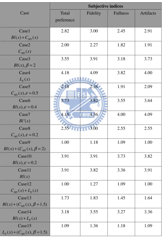
Table 6. The target output (listening test result) of the ANN. The first ten cases of objective index were selected as the target output data for training the ANN. The grading scale ranges from 1 to 5.

Case

Subjective indices

Total preference

Fidelity Fullness Artifacts

Case1 ( ) _MS( ) Bl x +C x 2.82 3.00 2.45 2.91 Case2 ( ) MS C x 2.00 2.27 1.82 1.91 Case3 ( ), 2 Bl x β = 3.55 3.91 3.18 3.73 Case4 ( ) E L x 4.18 4.09 3.82 4.00 Case5 ( ), 0.5 MS C x ε = 2.18 2.36 1.91 2.09 Case6 ( ), 0.4 Bl x ε = 3.73 3.82 3.55 3.64 Case7 '( ) Bl x 4.18 4.36 4.00 4.09 Case8 ( ), 0.2 MS C x ε = 2.55 3.00 2.55 2.55 Case9 ( ) ( _MS( ), 2) Bl x + C x β = 1.00 1.18 1.09 1.00 Case10 ( ), 0.2 Bl x ε = 3.91 3.91 3.73 3.82 Case11 ( ) Bl x 3.91 3.82 3.36 3.91 Case12 ( ) ( ) MS E C x +L x 1.00 1.27 1.09 1.00 Case13 ( ) ( _MS( ), 1.5) Bl x + C x β = 1.73 1.83 1.45 1.64 Case14 ( ) _E( ) Bl x +L x 3.18 3.55 3.27 3.36 Case15 ( ) ( ( ), 1.5) E MS L x + C x β = 1.09 1.36 1.18 1.09

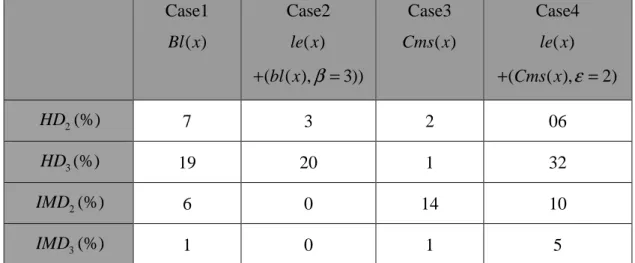
Table 7. Four nonlinear distortions, HD2 , HD3 , IMD2 and IMD3 , of the

out-group test as the ANN inputs based on the Loudspeaker model B. Case1 ( ) Bl x Case2 ( ) le x ( ( ),bl x β 3)) + = Case3 ( ) Cms x Case4 ( ) le x (Cms x( ),ε 2) + = 2 HD (%) 7 3 2 06 3 HD (%) 19 20 1 32 2 IMD (%) 6 0 14 10 3 IMD (%) 1 0 1 5

(a)

(b)

Fig. 1 Electroacoustic analogous circuit of a moving-coil loudspeaker. (a) The equivalent circuit. (b) The circuit of the thermal model.

P

V

T

TV

R

C

_TV M

T

M

T

∆

R

_TM

C

_TM V

T

∆

A

T

( ) E V R T L x_E( ) 2( ) L x 2( ) R x ( ) Bl x v Bl x i( ) ( ) MS C x M_MS R_MS F x i im( , , )2 u i 2 i v ( ) Bl x

Fig. 2 The flowchart of the modeling and verification procedure for the ANN-based loudspeaker assessment system

Loudspeaker A Large Signal

Model

Nonlinear Distortion Index

2, 3, 2, 3 HD HD IMD IMD Listening Tests Train ANN Loudspeaker B Large Signal Model

Nonlinear Distortion Index

2, 3, 2, 3 HD HD IMD IMD Listening Tests Trained ANN u(t) u(t) In-group Verification Out-group Verification e Subjective Attributes Subjective Attributes - Distortion type, Magnitude Subjective Attributes +

Fig. 3 The result of the listening test for the fifteen nonlinear loudspeaker models. The means and spreads (with 95% confidence intervals) of the grades are indicated in the figure. The x-axis and y-axis correspond to the nonlinear models and the grades, respectively.

Fig. 4 The schematic of the neuron. The symbol an is the input, wn is the

weight, b is the bias, and o is output.

a

1

w

1

w

2

w

n 1

o

n n n

net

=

∑

a w

+

b

a

2

a

n

…

b

Fig. 5 The structure of the back-propagation ANN. The symbol a is the hidden layer, a hidden layer of fifteen neurons, xi _{is the input layer of the nonlinear}

distortion measures HD HD IMD2, 3, 2 _and IMD3_, wij _and wk _{are the weights,} b1

and b2 _{are the bias units, and} y _{is the output of the subjective attributes: Fidelity,}

Fullness, Artifacts and Total Preference.

x

1

x

2

x

3

x

4

a

b

1

b

2

w

ij

w

k

y

1

y

2

y

3

y

4

Layer 1

(Input layer)

Layer 2

(Hidden layer)

Layer 3

(Output layer)

Bias unit

Bias unit

-10 -8 -6 -4 -2 0 2 4 6 8

case1 case2 case3 case4 case5

E rr or ( % )

Fidelity Fullness Artifacts Total Preference

Fig. 6 Comparison of Total preference, Fidelity, Fullness and Artifacts predicted by the ANN and the subjective data obtained from the listening test for the last five cases (in-group verification).

5

Output Target

Fig. 7 The out-group test result of the listening test for the four nonlinear

loudspeaker models. The means and spreads (with 95% confidence intervals) of the grades are indicated in the figure. The x-axis and y-axis correspond to the nonlinear models and the grades, respectively.

-15 -10 -5 0 5 10

case1 case2 case3 case4

E rr o r (% )

Fidelity Fullness Artifacts Total Preference

Fig. 8 The results of the out-group test of the ANN based on the Loudspeaker model B. Total preference, Fidelity, Fullness and Artifacts predicted by the ANN and the subjective data obtained from the listening test are compared.

5

Output Target

Fig. 9 The flow chart of the iterative procedure from FDM method for the coupled equation system

Fig. 10 Acoustical system includes the sound radiation, air gap, back chamber and acoustical holes influence.

Fig. 12 The comprehensive system combines the acoustical, mechanical and electrical system.