國立交通大學
多媒體工程研究所
碩 士 論 文
以光源對物體可見度為導向
之重要性取樣法
Visibility-Guided Importance Sampling
研 究 生:吳昱霆
指導教授:施仁忠 教授
以光源對物體可見度為導向之重要性取樣法
Visibility-Guided Importance Sampling
研 究 生:吳昱霆
Student:Yu-Ting Wu
指導教授:施仁忠
Advisor:Zen-Chung Shih
國 立 交 通 大 學
多 媒 體 工 程 研 究 所
碩 士 論 文
A ThesisSubmitted to Institute of Multimedia Engineering College of Computer Science
National Chiao Tung University in Partial Fulfillment of the Requirements
for the Degree of Master
in
Computer Science June 2009
Hsinchu, Taiwan, Republic of China
中華民國九十八年六月
I
以光源對物體可見度為導向之重要性取樣法
研究生:吳昱霆
指導教授:施仁忠 教授
國立交通大學多媒體工程研究所
摘
要
本論文在產生取樣點時考量光源與物體之間的可見度,提出一個新的重要性 取樣方法。本演算法將之前使用球面輻射基底函數(SRBF)考量 BRDF 與環境光 源的重要性取樣法做了延伸,藉由使用先前可見度測試的結果來調整每個球面輻 射基底的權重而將可見度的影響結合於重要性取樣函式(Importance Sampling Function)中。與先前許多在二維空間考量可見度關連性的重要性取樣法不同,本 演算法在三維空間中考量可見度的影響,避免重複地在先前可見度測試失敗的方 向上放置取樣點。因此較多的取樣點能通過可見度的測試而對最後繪製的結果產 生貢獻。在三維空間中考量可見度關連性將使我們的演算法更適用於一些大部分 光源為不可視的特殊場景。由結果可以看出來,本演算法大量的減少了整張畫面 的誤差與雜訊,而並不只是針對陰影邊緣而已。在花費相同時間下,本演算法所 產生的結果也遠優於先前未考慮可見度的方法。雖然我們的演算法是架構在以球 面輻射基底函數(SRBF)上,但是本論文的想法亦可被延伸至其它基底,像是小 波函數(Wavelet)或是球面調和函數(Spherical harmonics)。II
Visibility-Guided Importance Sampling
Student:Yu-Ting Wu
Advisor:Prof. Zen-Chung Shih
Institute of Multimedia Engineering
National Chiao Tung University
ABSTRACT
We propose a novel sampling algorithm by considering the importance of visibility in the sampling process. This algorithm extends the bidirectional importance sampling techniques based on SRBF representation by adjusting the weight of each SRBF basis according to the previous history in visibility tests, thus combing the visibility term into importance function. Unlike previous visibility-related researches in importance sampling exploit image-space visibility coherence, we consider visibility in object space by avoiding redrawing samples in invisible directions. Consequently more samples pass the visibility test and contribute to the final rendered result. Considering visibility in object space would make our algorithm more flexible, even for scenes which have heavy occlusion. Our approach successfully reduces the variance over the entire image, not only along the shadow boundaries. Under the same computing performance, we can obtain higher quality than previous bidirectional importance approaches. Although our proposed algorithm is based on the SRBF representation, it can also be applied to other basis such as wavelet or spherical harmonics.
III
Acknowledgement
First of all, I would like to thank to my advisor, Dr. Zen-Chung Shih, for his help and supervision in this work. Also, I thank for all the members of Computer Graphics & Virtual Reality Lab for their comments and instructions. Especially, I gratefully acknowledge the helpful discussions with Yu-Ting Tsai on several points in this thesis. Finally, special thanks go to my family and my dear friends, and the achievement of this work dedicated to them.
IV
Content
摘 要... I ABSTRACT ... II Acknowledgement ... III Content ... IV List of Figures ... V List of Tables ... VIIChapter 1 Introduction ... 1
1.1 Motivation ... 1
1.2 System Overview ... 3
1.3 Thesis Organization ... 4
Chapter 2 Related Work ... 6
2.1 Importance Sampling ... 7
2.2 Visibility Coherence ... 8
2.3 Visibility Sampling ... 9
Chapter 3 Background of SRBFs ... 11
Chapter 4 Algorithm ... 15
4.1 Product of the Illumination and BRDF ... 18
4.2 Exploiting Visibility Coherence ... 19
4.3 Taking Samples from SRBF ... 25
Chapter 5 Implementation Details ... 26
Chapter 6 Results and Discussion ... 29
Chapter 7 Conclusion and Future Work ... 49
V
List of Figures
Figure 1.1: A special scene ... 2
Figure 1.2: System Overview ... 4
Figure 3.1: 3D plot of a Gaussian SRBF ... 11
Figure 3.2 SRBF representation for a spherical function (k = 3) ... 12
Figure 4.1: Off-line fitting process ... 16
Figure 4.2: Run-time rendering process ... 17
Figure 4.3: Run-time example 1 ... 22
Figure 4.4: Run-time example 2 ... 22
Figure 4.5: Run-time example 3 ... 23
Figure 4.6: Run-time example 4 ... 23
Figure 4.7: Run-time example 5 ... 24
Figure 4.8: Run-time example 6 ... 24
Figure 4.9: The elevation angle and the azimuth angle defined against SRBF ... 25
Figure 6.1: The Uffizi Gallery environment map ... 29
Figure 6.2: “Buddh and Car” Scene ... 30
Figure 6.3: “Bathroom” Scene ... 30
Figure 6.4: “Meeting Room” Scene ... 31
Figure 6.5: “Restroom” Scene ... 31
Figure 6.6: Rendered results of “Buddha and Car” Scene using 200 samples/pixel ... 32
Figure 6.7: Rendered results of “Buddha and Car” Scene using 400 samples/pixel ... 33
Figure 6.8: Referenced image of the two zoom-in regions (“Buddha And Car” Scene) ... 34
Figure 6.9: Comparison of the first zoom-in region (“Buddha And Car” Scene) ... 34 Figure 6.10: Comparison of the second zoom-in region (“Buddha And Car” Scene) . 35
VI
Figure 6.11: RMS Error of the “Buddha And Car” Scene ... 36
Figure 6.12: Rendered results of “Bathroom” Scene ... 37
Figure 6.13: RMS Error of the “Bathroom” Scene ... 38
Figure 6.14: Rendered results of “Meeting Room” Scene ... 39
Figure 6.15: Referenced image of the two zoom-in regions (“Meeting Room” Scene) ... 40
Figure 6.16: Comparison of the first zoom-in region (“Meeting Room” Scene) ... 40
Figure 6.17: Comparison of the second zoom-in region (“Meeting Room” Scene) .... 41
Figure 6.18: Root Mean Square (RMS) Error Comparison of “Meeting Room” Scene ... 42
Figure 6.19: Equal-samples rendered results of “Restroom” Scene ... 43
Figure 6.20: Referenced image of the two zoom-in regions (“Restroom” Scene) ... 43
Figure 6.21: Equal-samples Comparison: The first zoom-in region (“Restroom” Scene) ... 44
Figure 6.22: Equal-samples Comparison: The second zoom-in region (“Restroom” Scene) ... 44
Figure 6.23: Equal-samples Comparison: Root Mean Square (RMS) Error of “Restroom Scene” ... 45
Figure 6.24: Equal-time rendered results of “Restroom” Scene ... 46
Figure 6.25: Equal-time Comparison: The first zoom-in region (“Restroom” Scene) 46 Figure 6.26: Equal-time Comparison: The second zoom-in region (“Restroom” Scene) ... 47
Figure 6.27: Equal-time Comparison: Root Mean Square (RMS) Error of “Restroom” Scene ... 47
VII
List of Tables
Table 6.1: Variance comparison of “Buddha And Car” Scene ... 36 Table 6.2: Variance comparison of “Bathroom” Scene ... 38 Table 6.3: Variance Comparison of “Meeting Room” Scene ... 41 Table 6.4: Equal-samples Comparison: Variance Comparison of “Restroom” Scene . 45
1
Chapter 1 Introduction
1.1 Motivation
Monte Carlo ray tracing [10] is widely used in global illumination. This kind of algorithms has several advantages over finite element method (radiosity), such as no additional tessellation is necessary and any type of materials can be handled. Besides, current hardwares also have better support to this method. However, brute force Monte Carlo ray tracing based on random sampling often takes too much time to get satisfying results and produces undesired noise along shadow boundaries.
To improve the efficiency of brute force Monte Carlo ray tracing and reduce the variance, the concept of importance sampling was first proposed by Ward [31] in 1992 and becomes a popular variance-reduction method. Instead of distributing samples randomly, importance sampling concentrates the samples in regions which have large integral values in the rendering equation, namely, the important regions. By using importance sampling, we can obtain better result with fewer samples.
Although the topic of importance sampling has been studied for twenty years, estimating the integral of the triple product, illumination, BRDF, and the visibility function in the rendering equation, is still an elusive goal. The major difficulty is that the visibility function can only be determined in run time. Most importance sampling algorithms ignore visibility and only draw samples based on the product of illumination and BRDF terms, such as Tsai et al. [27] and Clarberg et al. [4]. Their
2
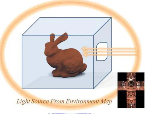
algorithms work well in general scenes; however, in some particular scenes in which the visibility term dominates the importance function, these approaches still produce large variance. Recently some researches [5][7] use image-space coherence or control variate to reduce the variance. Nevertheless, consider Figure 1.1, a room with the only light source coming from windows, the image-space coherence is hard to be exploited.
Figure 1.1: A special scene. The light source from environment map (orange ring) can only come from the window on the wall, and the visibility term will dominate the integral in rendering equation
The goal of our research is to propose a visibility-guided importance sampling algorithm which considers the visibility between surfaces and light source in the progress of sampling. In the run-time process, we avoid distributing samples along the directions which the previous visibility tests failed, thus increasing the possibility of sampling along visible directions. Our algorithm considers visibility in object space in the run-time sampling process. It still works very well in both general scenes and the
3
scenes like Figure 1.1. In the following paragraphs, we summarize our major contribution:
1. Instead of exploiting visibility coherence in the image-space, we combine the visibility function into importance function in the run-time sampling process. 2. Our algorithm does not need any additional passes; it considers visibility in
the original sampling process. Moreover, all the additional resource we need is a small-size buffer.
3. Our proposed idea can be easily combined with previous product sampling algorithms and improve the sampling efficiency.
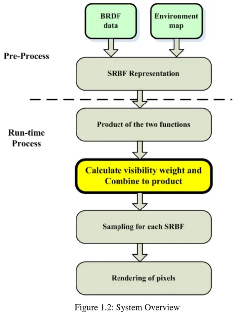
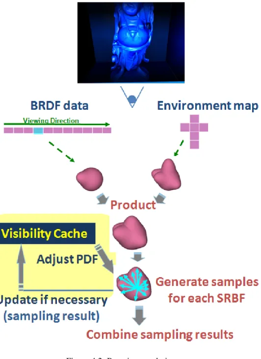
1.2 System Overview
Figure 1.2 gives an overview of our system. Our system is similar to the one proposed by Tsai et al. [27], which is a product importance sampling algorithm using SRBF representation. We develop our visibility-guided importance sampling algorithm based on Tsai’s system by adding a step to consider the visibility (The yellow step in Figure 1.2).
In Tsai’s system, they first fit BRDF data and environment map into SRBFs in preprocess. Then, in the run-time process, the products of SRBFs are evaluated to determine how many samples each SRBF should take. To take visibility into consideration, we use previous history of visibility test to evaluate a visibility weight. The weight is then used to adjust the probability of choosing which SRBF for sampling. To avoid invisible directions, the SRBFs with their centers close to previous
4
invisible directions will have less possibility to be chosen. After the visibility-guided adjustment, we use Tsai’s method to generate samples from each SRBF and render the final image.
Figure 1.2: System Overview
1.3 Thesis Organization
The rests of this thesis are organized in the following manner. Chapter 2 reviews some of the related works in importance sampling and visibility sampling. In Chapter 3, we briefly introduce the background knowledge of SRBFs. In Chapter 4, we
5
present the main concept of our visibility-guided importance algorithm. The implementation details will be demonstrated in Chapter 5. Chapter 6 shows the result of our algorithm. We also make comparisons toward previous works and give some discussion in this chapter. Finally, we conclude our work and propose some future works in the Chapter 7.
6
Chapter 2 Related Work
In this chapter, we review previous works on importance sampling and visibility sampling. As mentioned before, importance sampling is a popular approach to improve the performance of Monte-Carlo methods. The major concept of importance sampling is to concentrate the sampling efforts on important regions. If important samples are generated more frequently, the variance can be greatly reduced even with fewer samples. Ideally, the number of samples should be proportional to the rendering equation:
(
)
(
)
(
i o) (
i i) (
i)(
i)
i o e od
n
x
V
x
L
x
B
x
L
x
L
ω
ω
ω
ω
ω
ω
ω
ω
⋅
+
=
∫
Ω,
,
,
,
,
,
(1) where L (x,ω denotes the outgoing radiance from a surface point x in viewing o) direction ω , o L is the incident radiance, B is the BRDF, V is the visibility relation i
between the incident light and surface, and finally n is the surface normal at x .
Combing with Monte-Carlo estimator and considering the importance functionPr
(
ωi,n|x,ωo)
, the equation becomes:(
)
(
)
(
)
(
)
(
)
∑
=⋅
+
=
N n in o i n i n i i o n i o e ox
n
x
V
x
L
x
B
N
x
L
x
L
1 , , , ,,
|
Pr
,
)
,
(
)
,
,
(
1
,
,
ω
ω
ω
ω
ω
ω
ω
ω
ω
(2)
The major difficulty in importance sampling is to estimate the integral of the triple product ofL ,i B, and V as soon as possible in run time. For performance reason, previous importance sampling algorithms usually transform the BRDF data and environment maps into different basis such as spherical harmonics, wavelets, or
7
spherical radial basis functions. The bases are then used to evaluate the value of importance function Pr
(
ωi,n|x,ωo)
in run time. BRDF importance sampling methods distribute samples according to the BRDF distribution; Environment map importance sampling techniques concentrate samples at regions having large value in incident radiance function; Product importance sampling approaches evaluate the product of BRDF and illumination in run time and determine sampling density according to the value of product. However, considering visibility during sampling would encounter problems discussed in the next paragraph.The simplest idea is to combine the visibility estimation V~ into the importance function and calculate importance by evaluating the triple product L~iB~V~. However, this approach requires V~ ≠0 wherever V ≠0 because V~ ≠0 will stop the exploration directly and lead to bias. Moreover, visibility could only be determined in run time. This means that the estimation is hard to be generated. For these reasons, the visibility term is usually ignored in the importance sampling algorithms. To solve this problem, we present a novel approach to consider visibility during drawing samples.
2.1 Importance Sampling
Pioneered by Ward [31], the research of importance sampling starts from considering one of the term B or L . In the research of BRDF importance sampling, i
Lafortune [15] used multiple cosine-lobes for representing the BRDF. Lalonde [16] used wavelets to represent the measured BRDF. Matusik [18] also used wavelets to represent BRDF and presented a numerical sampling method based on reparameterizing the BRDF by using half-angle. Weng and Shih [32] fit the measured
8
SRBF data into scattered SRBFs and estimated the probability distribution for importance sampling. In the research of environment map importance sampling [22] [23], the environment maps were transformed into finite basis function such as wavelets or spherical harmonics.
Recently several researches have worked on drawing samples from the product distribution of the incident radiance function and the BRDF. For general scenes, these approaches produce high-quality images with small number of samples. Burke et al. [2] introduced a bidirectional sampling technique based on sampling-importance re-sampling (SIR). Clarberg et al. [3] used a hierarchical wavelet representation to estimate the product distribution of BRDF and illumination, later they [4] modified their algorithm by fast quad-tree product in run-time. Tsai et al. [27] proposed a product importance sampling algorithm using SRBF representation. Although these researches work well in general scenes, the lack of considering visibility makes them produces large variance in the scenes like Figure 1.1. Rosusselle et al. [24] proposed a visibility approximation method in their product importance sampling algorithm. However, their approximation needed the simplification of meshes and a hierarchical structure of each function. Huang et al. [9] considered visibility by using more samples for partial-occluded regions. They do not take visibility into importance function.
2.2 Visibility Coherence
9
sampling. Ghosh et al. [7] presented a two-stage importance sampling algorithm to reduce the noise along the shadowed regions. They first used product importance sampling to create a visibility mask for marking the partially occluded pixels, then they use metropolis sampling to exploit the visibility coherence in image space. Their work successfully reduced the variance along the shadowed regions for general scenes. However, if most directions are invisible, the image-space coherence is hard to exploit and unreliable.
Donikian et al. [6] used an adaptive importance sampling approach to iteratively refine the importance function, the image is divided into 8 x 8 blocks and refined iteratively. Hart et al. [8] used a lazy visibility evaluation to compute direct illumination, spatial visibility coherence was exploited by a flood-fill algorithm. Clarberg et al [5] analyzed the visibility coherence and used control variate to reformulate the rendering equation. They placed visibility records in the scene, and then used linear interpolation of records to estimate the visibility based on normal difference and distance. Compared to two-stage importance sampling, their work reduced the noise of the entire image. Although they used control variate to exploit the visibility coherence in three-dimensional space, they did not combine the visibility into importance function during sampling. Moreover, their approach needs lots of visibility records in complex scene, becoming memory-consuming and time-consuming for the computation of records.
2.3 Visibility Sampling
10
not an importance sampling algorithm, their algorithm has many ideas similar to our work. Their strategy was to cast rays which are likely to sample new triangles in the ray-space and thus improving the sampling efficiency. Our algorithm also uses this concept in importance sampling. We avoid redrawing samples which are likely to be invisible.
11
Chapter 3 Background of SRBFs
In this chapter, we introduce the backgrounds of Spherical Radial Basis Function (SRBF). It has been shown in data analysis by Weng and Shih [32] that SRBF is more appropriate for modeling spherical data, such as BRDF or incident radiance function than other basis. Spherical data can be represented by SRBFs without any artificial boundaries or distortions. It also has many useful properties, such as rotational invariance and positive definiteness. For these reasons, we develop our proposed visibility-guided importance sampling algorithm based on the SRBF representation.
The spherical radial basis functions (SRBFs) are special radial basis functions defined on the unit sphere. It is recognized as a circularly axis-symmetric reproducing kernel function defined on m
S (unit sphere in m+1
R ). The kernel functions only depend on the spherical distance between two unit vectors. Figure 3.1 shows the 3D plot of a Gaussian SRBF example.
Figure 3.1: 3D plot of a Gaussian SRBF
Bandwidth
Center
12
Let η and ξ be two points on m
S and θ(η, ξ) be the geodesic distance between η and ξ on Sm, i.e. the arc length of the great circle joining the η and ξ. The kernel functions of SRBFs will depend on θ and can be expressed in the expansions of Legendre polynomials:
(
)
(
)
∑
∞(
)
=⋅
=
⋅
=
0cos
l l lP
G
G
G
θ
η
ξ
η
ξ
(3)where Pl
(
η ⋅ξ)
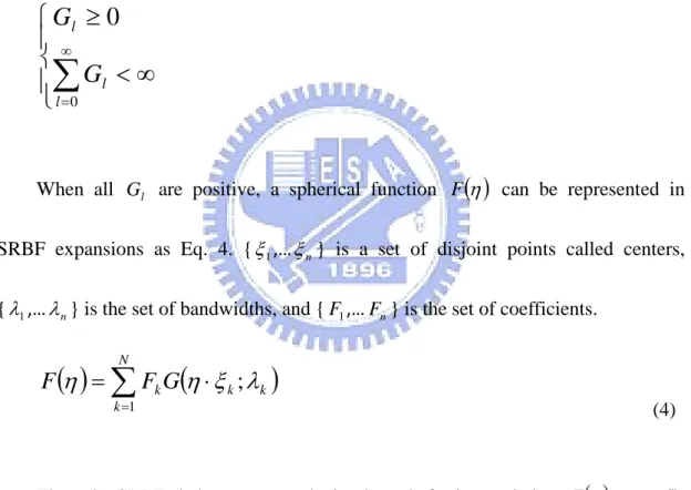
is the Legendre polynomials of degree l , and G is the Legendre lcoefficients satisfying the following two conditions:
∞
<
≥
∑
∞ =00
l l lG
G
When all G are positive, a spherical function l F
( )
η can be represented in SRBF expansions as Eq. 4. {ξ1,…ξn} is a set of disjoint points called centers, {λ1,…λn} is the set of bandwidths, and {F ,…1 F } is the set of coefficients. n( )
∑
(
)
=⋅
=
N k k k kG
F
F
1;
λ
ξ
η
η
(4)Thus, the SRBFs behave as reproducing kernels for interpolating F
( )
η on Sm. Figure 3.2 shows an example of SRBF representation for a spherical function F( )
η .13
Since SRBF can be expressed in terms of expansions in Legendre polynomials, it facilitates the evaluation of convoluting two SRBFs. We can easily calculate the spherical singular integral based on the orthogonal property of Legendre polynomials in [-1, 1]:
(
)(
)
(
) (
)
( )
(
)
,
0 2 1 , 2 1 2 1 2 1 2 1∑
∫
∞ =⋅
=
⋅
⋅
=
⋅
∗
l l l m m l l S mP
d
G
G
d
H
G
G
G
mξ
ξ
ω
η
ω
ξ
η
ξ
η
ξ
ξ
(5) where ωm is the total surface area of mS , dm,l is the dimension of the space of order-l spherical harmonics on m
S , and d denotes the differential surface element ω
on Sm. Please refer to [19] for more details about spherical radial basis functions.
The Gaussian SRBF kernel is an example of SRBFs. Its kernel is defined as follows:
(
η
⋅
ξ
;
λ
)
=
−λ λ( )η⋅ξ,
λ
>
0
,
e
e
G
Gau (6)We adopt Gaussian SRBF kernel as the kernel function based on the following reasons. First, Tsai and Shih [22] have proved that the convolution of two Gaussian SRBFs has a mathematically simple form for small m. It can be written as:
(
)
(
)
(
)
( )
2 1 2 1 2 1 2 1 2 12
2
1
,
;
2 1 − − + −
+
Γ
=
⋅
∗
m m m Gau m Gaur
r
I
m
e
G
G
ω
λ
λ
λ
λ
ξ
ξ
(7) where r=λ1ξ1 +λ2ξ2. Second, the product of two Gaussian SRBFs is easy to evaluate. For more details about the proof of the Eq. 7, please refer to [25].14
We use SRBFs to represent the BRDF data and the environment maps. As introduced above, the product of BRDF and illumination represented in SRBFs can be fast evaluated in run time. Our algorithm then computes a visibility weight to adjusting the weight of the product, thus combing the visibility function into importance function. We will demonstrate our major concept in next chapter.
15
Chapter 4 Algorithm
We develop our visibility-guided importance sampling algorithm based on the product importance sampling algorithm proposed by Tsai et al. [27]. In their original system, BRDF data and environment maps are fit into SRBF representation in the pre-process and the product of the SRBFs are evaluated to determine how many samples that each SRBF should take in run time. As usual product importance sampling approaches, they do not consider the visibility function during sampling. We enhance their system by introducing a visibility term into the importance function.
The major idea of our approach is to generate new samples based on old ones. In the sampling process, we keep the history of visibility test in a cache for each hit point on the surface by Monte Carlo ray tracing. The cache stores all the previous invisible directions for the point. When taking the next sample, we can use this information to avoid redrawing samples along the invisible directions. As a result, the number of samples which pass the visibility test increases and the sampling efficiency is improved.
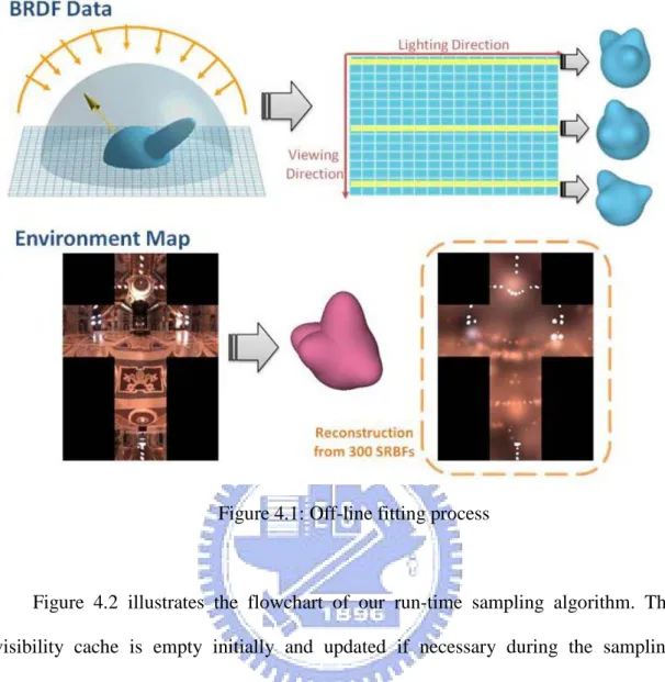
Figure 4.1 illustrates the off-line fitting process. We use Tsai’s off-line fitting algorithm to fit the BRDF data and environment map into SRBFs. For the BRDF data, each viewing direction is fit into SRBFs respectively. For the environment map, the total environment map is represented as a multiple kernel SRBF. These SRBFs are then used in run time to evaluate the importance function.
16
Figure 4.1: Off-line fitting process
Figure 4.2 illustrates the flowchart of our run-time sampling algorithm. The visibility cache is empty initially and updated if necessary during the sampling process. When a view ray hits an object in the scene, the product of the BRDF data and environment map represented in SRBFs are evaluated and a multiple kernel SRBF is generated. Instead of determining the number of samples on each SRBF directly according to the value of coefficient, we fetch the previous sampling history from cache for obtaining which directions failed in the previous visibility tests. If the cache is not empty, the history is used to adjust the probability of SRBFs. A SRBF with its center close to the invisible direction will have lower probability to be chosen. After this adjustment, we determine the number of samples taking from each SRBF and generate samples according to each SRBF. Finally the sampling results are combined for determining the outgoing radiance along the camera ray.
17
Figure 4.2: Run-time rendering process
The following sections are organized as follows. In section 4.1, we explain how the product of BRDF and illumination is evaluated. In section 4.2, we describe how we maintain the visibility information and adjust the weight for choosing SRBF. We also use an example to illustrate how our algorithm works. Finally in section 4.3 we describe how we generate samples according to a SRBF.
18
4.1 Product of the Illumination and BRDF
We use Tsai’s method to estimate the product of the illumination and BRDF represented in SRBFs. As mentioned before, the product of two Gaussian SRBFs can be easily computed as follows:
( ) ( ) ( ) 3 2 2 2 1 3 2 2 1 1 3 2 1 3 3 2 1 3 3 2 2 1 1
λ
ξ
λ
ξ
λ
ξ
ξ
λ
ξ
λ
λ
ξ η λ ξ η λ ξ η λ+
=
+
=
⋅
=
=
⋅
⋅ ⋅ ⋅F
F
F
e
F
e
F
e
F
where F is the coefficient of product result, 3 λ3 is the bandwidth of product result, and ξ is the center of the product result. The product of N SRBFs from BRDF data 3 and M SRBFs from illumination is shown as follows:
( ) ( )
∑
(
)
∑
(
)
= =⋅
⋅
≈
N n n n i brdf n M m m m i on illuminati m i iB
F
G
F
G
L
o 1 1;
;
λ
ω
ξ
λ
ξ
ω
ω
ω
ω (8) where L( )
ω is the incident radiance and i( )
io
Bω ω is the BRDF with a fixed outgoing direction ω . o
After calculating the product, the total number of SRBFs becomes M x N. For performance issue, we only keep n SRBFs with larger coefficient and prune the rests. Because most energy is distributed in SRBFs with large coefficient, we can get a good approximation by keeping these n functions. For more details, please refer to Tsai’s paper [27].
19
4.2 Exploiting Visibility Coherence
After calculating the product of the SRBFs, we will have multiple SRBF kernel functions. Now we must decide how many samples should be taken from each SRBF kernel. We employ the mixture model for taking samples from the SRBFs. To generate a new sampling direction, we first select a SRBF l with probabilityP(l). Then we generate a sampling direction for shadow ray against the center of SRBF. In the original Tsai’s paper, P(l) is determined by
∑
==
n i i lI
I
l
P
1)
(
where I is the integral of SRBF i. The integral represents the total energy gathered i
from all directions. Therefore, the meaning of Eq. 9 is to allocate samples according to the energy of each SRBF with respect to the total energy of all SRBFs.
To consider the visibility, we introduce a visibility term V into Eq. 9. The i
probability of choosing the SRBF l from the multiple SRBF kernel functions
becomes:
∑
==
n i i i l lI
V
I
V
l
P
1)
(
the visibility term V stands for the visibility weight of the SRBF i . It is determined i
according to the previous sampling history. In the following, we will demonstrate how to keep the history and derive the visibility weight.
To build the history, we create a visibility cache to keep a list of invisible directions for shadow rays. In the original Monte Carlo ray tracing algorithm, several
20
shadow rays are generated sequentially to sample the lighting contribution from the environment map when a view ray hits the scene object. Then the average is calculated as the outgoing radiance along the camera ray. Our algorithm takes advantage of this sequential property. If the sampling direction fails in the visibility test, we record its direction in the cache. When taking next sample, the content in the cache is used to adjust the probability P(l) of each SRBF. By keeping the results of visibility tests in visibility cache, we can avoid redrawing samples in invisible directions with respect to this ray-tracing point. We define the visibility term as follows: k l
dir
Num
V
∝
)
(
1
where Num(dir) represents the number of directions which are close to the center of the SRBF l , and k is a constant to control the decreasing slope.
For each SRBF l , we determine whether the invisible directions in the visibility
cache and the center of SRBF are close or not. If the angle between these two directions is smaller than a threshold, we increase Num(dir). This will lower the visibility term V , meaning the SRBFs with their centers close to the invisible l
directions will have smaller probability to be chosen. Now the problem is how to determine the threshold? Instead of using a fixed threshold, we construct a bandwidth function to determine the threshold. We assume the angle between the center of a SRBF and an invisible direction in the visibility cache is a normal distribution, we can evaluate the standard deviation of angle with some appropriate simplification as follows: 2 / 1 2 0 2
=
∫
−dx
e
x
Lns
Bxσ
(9)21
where x is cosine value of the angle between two directions, B is the bandwidth of
the SRBF, and Lns is a normalization term which can be calculated as:
1 2 0 − −
=
∫
e
dx
Lns
Bx (10)The bandwidth represents the influence of the SRBF. We can use the standard deviation to cut a fixed percentage of directions from different SRBF by evaluating the bandwidth function.
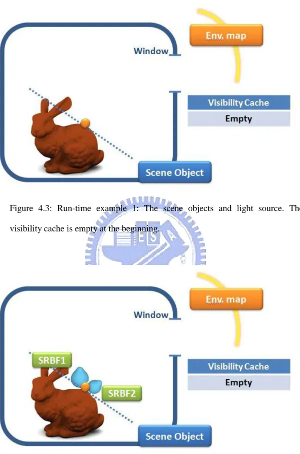
Now consider Figures 4.3 ~ 4.8, we show an example to explain how our algorithm works. Figure 4.3 shows a scene with a bunny in a room. Light sources coming from environment map can only illuminate the scene through the window on the wall. The visibility cache is empty initially and updated through the progress of sampling. As shown in Figure 4.4, when a view ray hits the surface, we first evaluate the product of BRDF and illumination to generate a multiple kernel SRBF. As shown in Figure 4.5, since at beginning the visibility cache is empty, the SRBF with larger coefficient among the multiple kernel functions has higher probability to be chosen (SRBF1 in Figure 4.5). A sampling direction is then generated from SRBF1. In Figure 4.6, the direction fails in visibility test. We record its direction (Direction1 in Figure 4.6) in the visibility cache. When we continue to generate the next sample, the visibility cache is used to adjust the coefficient of SRBFs. As shown in Figure 4.7, the coefficient of SRBF1 is reduced so that we have higher probability to select SRBF2 for sampling. Finally, as shown in Figure 4.8, since Direction2 passes the visibility test, we do not need to update the cache. From this example, we can conclude that more samples are concentrated in the visible directions like Direction2.
22
Figure 4.3: Run-time example 1: The scene objects and light source. The visibility cache is empty at the beginning.
Figure 4.4: Run-time example 2: Multiple SRBF kernel functions are generated for a ray-tracing hit.
23
Figure 4.5: Run-time example 3: The visibility cache is empty and the SRBF with larger coefficient has higher probability to be chosen. An illumination sampling ray is then generated according to the SRBF.
Figure 4.6: Run-time example 4: The ray generated from SRBF1 fails in the visibility test. Its direction is then recorded in the cache.
24
Figure 4.7: Run-time example 5: When taking next sample, the content in the visibility cache is used to lower the probability of SRBF1. As a result, SRBF2 has higher probability to be chosen.
Figure 4.8: Run-time example 6: The ray generated from SRBF2 (Direction2) passes the visibility test. Therefore, there is no need to update the cache.
25
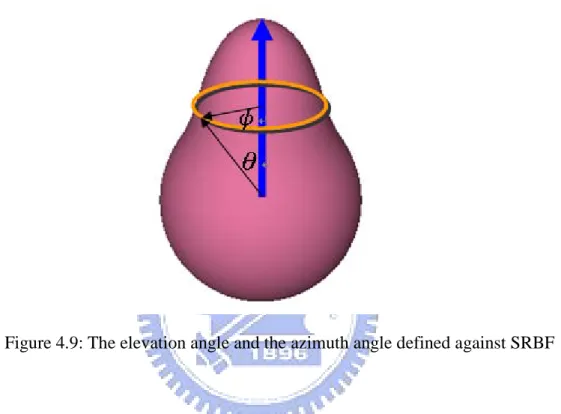
4.3 Taking Samples from SRBF
After having chosen which SRBF for sampling, we generate the sampling direction from the SRBF kernel by sequentially selecting the elevation angle θ and azimuth angle φ (Figure 4.9).
Figure 4.9: The elevation angle and the azimuth angle defined against SRBF
We use metropolis random walk algorithm to determine the elevation angle θ with a desired density. For the azimuth angle φ, we simply generate a random number in [0. 2π] since SRBF is symmetric with respect to its center. After deciding these two angles, we can generate a sampling direction according to the SRBF.
The entire sampling process matches the concept of mixture model. To sample an illumination direction, we first select a SRBF l with probability P(l), and then generate an illumination direction d from the SRBF by the above approach.
26
Chapter 5 Implementation Details
We use the PBRT [21] system and path-tracing algorithm [12] to implement the Monte Carlo ray-tracing. While sampling, multiple rays are generated for each pixel from the camera. The outgoing radiance along these camera rays are gathered and combined by the Monte Carlo estimator. Once a camera ray intersects with objects in the scene, several directions are generated to sample the lighting contribution from the environment map. Our algorithm exploits the three-dimension visibility coherence in this stage: For n sampling directions at a hit point, we create a visibility cache to store the invisible directions. Compared with previous approaches, the size of the cache is all the additional memory space we need, which is negligible. Since the cache can be cleared and reused for each intersection, our approach does not need lots number of caches as Clarberg et al. [5]. Algorithm 5.1 shows the pseudo code of our algorithm, the major part to exploit visibility coherence is marked in the green rectangle. In the following paragraphs, we will give the implementation details of each step.
In preprocess, we fit the BRDF and environment data into SRBFs using Tsai’s approach [27]. In the run-time rendering process, for each camera ray shot from pixel, we use haar evaluation to get the closest BRDF data fit in preprocess. Then we compute the product of the SRBFs from BRDF and illumination to generate a multiple kernel SRBF. Now we have to determine how many samples each SRBF should take. As mentioned in the previous paragraph, we consider visibility by using the visibility cache. We use the content in the visibility cache and the formula shown in Chapter 4 to adjust the coefficient of each SRBF.
27
After finishing the adjustment, we calculate a one-dimensional cumulative density function (CDF) over the probabilities of the SRBFs. Then a random number between [0, 1] is used to traverse the CDF to determine which SRBF being chosen for taking sample. We then evaluate the rendering equation with the sampling direction and update the visibility cache if necessary: if the direction failed in the visibility test. This procedure will repeat until the computation of n sampling directions for shadow rays completes. The lighting contributions of n sampling directions are then averaged to determine the outgoing radiance along the camera ray. Finally, the results of m camera rays are combined by Monte Carlo estimator.
It is noted that the CDF should only be reconstructed when the visibility cache is updated. If previous sampling direction passed the visibility test, the coefficient of each SRBF does not need to be updated. We use a flag to control whether the CDF needs reconstruction. If the size of visibility cache gets large compared with previous run, we set the flag to be true to reconstruct the CDF. This approach will reduce the number of CDF reconstructions and improve the performance.
28
Preprocess
Fit BRDF and Environment map into SRBFs
Run-time
For each pixel, generate m camera rays
For camera rays 1 to m, if it has intersection with the scene object: Use Haar Evaluation to get the closest BRDF data
represented in SRBFs according to the camera ray
Compute the product of SRBFs from BRDF data and environment map
Repeat n times (n sampling direction)
Use the content in visibility cache to adjust the weight of each SRBF
Construct a CDF over the SRBFs and traverse a random number to select a SRBF for sampling
Generate a sampling direction according to the selected SRBF
Update the visibility cache if necessary
Average the n sampling results to evaluate the outgoing radiance along the camera ray
Combine the results of m camera rays by the Monte-Carlo estimator Combine the results of each pixel and get the rendered result
29
Chapter 6 Results and Discussion
This chapter first demonstrates the results of our algorithm. We implement our algorithm on a desktop PC with Intel Core2 Extreme CPU X9650, 8G RAM, and NVIDIA GeForce 8800 GTS 512 video card. We use several measured BRDF data from MERL and Cornell libraries and complex HDR environment maps for rendering. Each viewing direction of the materials is fit into 20 SRBFs and the environment maps are represented by 100 SRBFs.
In the following, we will compare our results with SRBFs-based product importance sampling presented by Tsai et al. [27]. These results are compared in equal-sample or equal-time manners. We use the Uffizi Gallery environment map (Figure 6.1) as light source and four different testing scenes (Figures 6.2 ~ 6.5). All the scenes are rendered with 5 shadow rays.
30
Figure 6.2: “Buddh and Car” Scene: “Mystique” Buddha, “GarnetRed” Car, and Cayman Walls
Figure 6.3: “Bathroom” Scene: “OrangePaint” Basket, “Teflon” Bathtub, and “WhitePaint” Walls
31
Figure 6.4: “Meeting Room” Scene: All the objects in the scene use “Fruitwood241” from MERL library as material
Figure 6.5: “Restroom” Scene: “Cayman” Bed, “GarnetRed” Closet, and “Teflon” Walls
32
We first compare the rendered results of “Buddha and Car” Scene. Figures 6.6 ~ 6.7 show the comparison of equal-samples results. We can find that our results are much brighter than the ones rendered with previous method. The reason is that shadow rays are concentrated along the visible directions. More of them pass the visibility test and contribute to the outgoing radiance.
33
Figure 6.7: Rendered results of “Buddha and Car” Scene using 400 samples/pixel
Figures 6.8 ~ 6.10 show the closer-look of the results. We can obviously find the reduction of noise in the two regions by comparing the images with the referenced image.
34
Figure 6.8: Referenced image of the two zoom-in regions (“Buddha And Car” Scene)
35
Figure 6.10: Comparison of the second zoom-in region (“Buddha And Car” Scene)
Then we compute the root mean square (RMS) error and variance with the referenced image. The results are displayed in Figure 6.11 and Table 6.1. In Figure 6.11, we use different colors to represent the error. Red means high error and blue means low. We can obviously find the decrease of red and yellow regions. Another important point we can find is that although we increase the number of samples per pixel from 200 to 400, the overall error does not decrease as expected in the Tsai’s results. The reason is most of the samples failed in the visibility tests and do not contribute to the final image. Our algorithm does not suffer this bottleneck and successfully reduces the error as the number of samples increases.
36
Figure 6.11: RMS Error of the “Buddha And Car” Scene. Red represents high error and blue represents low error. The higher-error regions (red and yellow) are reduced by using our approach
Tsai et al.[2008] Our method 200 samples/pixel 0.149487 0.081025 400 samples/pixel 0.139078 0.058851
Table 6.1: Variance comparison of “Buddha And Car” Scene
Then we compare the rendered results of the “Bathroom” Scene. In this scene, we use the measured BRDF data from MERL library for rendering. The scene is composed of an “OrangePaint” basket, a “Teflon” basetub, and “WhitePaint” Walls. Figure 6.12 shows the rendered results using different number of samples per pixel and 5 shadow rays per camera ray.
37
Figure 6.12: Rendered results of “Bathroom” Scene
Figure 6.13 and Table 6.2 shows the RMS error and variance of the “Bathroom” Scene. We can find the error near the bathtub and the entire variance is reduced.
38
Figure 6.13: RMS Error of the “Bathroom” Scene
Tsai et al.[2008] Our method 200 samples/pixel 0.155543 0.139747 400 samples/pixel 0.124805 0.103070
Table 6.2: Variance comparison of “Bathroom” Scene
Figure 6.14 shows the rendered results of “Meeting Room Scene” using Tsai’s and ours approach with 200 ~ 800 samples per pixel. The number of shadow rays generated for each camera ray is fixed to 5.
39
Figure 6.14: Rendered results of “Meeting Room” Scene
As shown in Figure 6.14, the results rendered with our algorithm are much brighter across the entire image. Moreover, Figures 6.15 ~ 6.17 show that our approach keeps more high-frequency details than previous method. Figure 6.15 shows the referenced image of the two zoom-in regions, and Figures 6.16 ~ 6.17 compares the rendered
40
results.
Figure 6.15: Referenced image of the two zoom-in regions (“Meeting Room” Scene).
41
Figure 6.17: Comparison of the second zoom-in region (“Meeting Room” Scene)
The RMS and variance of these two approaches are displayed in Figure 6.18 and Table 6.3. We can find the great reduction of variance from Table 6.3. Even with one-fourth samples, our proposed algorithm still produces less variance than the previous method. In the next scene, we will compare the equal-time rendered results of our approach and the one proposed by Tsai et al. [24].
Tsai et al.[2008] Our method 200 samples/pixel 0.127465 0.091346 400 samples/pixel 0.118740 0.068415 800 samples/pixel 0.106096 0.045513
42
Figure 6.18: Root Mean Square (RMS) Error Comparison of “Meeting Room” Scene
Finally consider the “Restroom” Scene. We first compare the equal-samples results as above. The rendered images are illustrated in Figure 6.19 and the zoom-in details are shown in Figures 6.20 ~ 6.22. The RMS error and variance are shown in Figure 6.23 and Table 6.4.
43
Figure 6.19: Equal-samples rendered results of “Restroom” Scene
44
Figure 6.21: Equal-samples Comparison: The first zoom-in region (“Restroom” Scene)
Figure 6.22: Equal-samples Comparison: The second zoom-in region (“Restroom” Scene)
45
Figure 6.23: Equal-samples Comparison: Root Mean Square (RMS) Error of “Restroom Scene”
Tsai et al.[2008] Our method 200 samples/pixel 0.125262 0.062662 400 samples/pixel 0.118084 0.047234
Table 6.4: Equal-samples Comparison: Variance Comparison of “Restroom” Scene
Then we use Figures 6.24 ~ 6.27 to show the equal-time results. Although our algorithm spends more time on each sample, we can obtain higher-quality images by using much fewer samples. The enhancement of performance is obvious as follows.
46
Figure 6.24: Equal-time rendered results of “Restroom” Scene
Figure 6.25: Equal-time Comparison: The first zoom-in region (“Restroom” Scene)
47
Figure 6.26: Equal-time Comparison: The second zoom-in region (“Restroom” Scene)
Figure 6.27: Equal-time Comparison: Root Mean Square (RMS) Error of “Restroom” Scene
48
The major overhead of our algorithm is the increase of frequency to reconstruct the CDF. However, it is interesting that the enhancement of quality is also positively proportional to the number of reconstruction. Since we only reconstruct the CDF when there is a new invisible direction recorded in the visibility cache, it seems that we can avoid the invisible directions more accurately if we have more contents in the cache. For general scenes which have little occlusion, our algorithm is as fast as Tsai et al. [27]. Because most of the time the visibility cache is empty, our algorithm works similarly as Tsai’s algorithm. We will have a little enhancement along the shadowed regions by spending a little more time (2% overhead). For the scenes like Figures 6.2 ~ 6.5, our algorithm increase 40% ~ 50% computation time compared with Tsai’s approach. However, as seen from Figures 6.24 ~ 6.27, we can obtain much better results by using the same time. Therefore, our proposed algorithm greatly improves the sampling efficiency.
49
Chapter 7 Conclusion and Future Work
We propose a novel algorithm to consider visibility in importance sampling based on the SRBF representation. Our algorithm considers visibility in object space by avoiding redrawing samples along the invisible directions. Compared with previous importance sampling techniques, our approach reduces the variance across the entire image, not only along the shadow boundaries. Furthermore, our approach does not need any other additional rendering pass and pre-computation of mesh. The only additional resource needed is a cache whose cost is negligible. As shown in the results, our approach greatly reduces the variance in the equal-time comparison.Although we implement our visibility-guided importance algorithm based on SRBF representation, this concept can be easily applied and implemented on other basis such as wavelet or spherical harmonics. No matter what basis we use, we just need to use the visibility cache to adjust the weight of each basis function in the run-time sampling process. Because the major concept of our algorithm is to avoid invisible directions while sampling and all the additional resource we need is a cache, it does not matter how the BRDF and illumination are represented.
In the future, we would use better data structures for our visibility cache to improve the performance. We also can combine the two-stage approach proposed by Ghosh et al. [7] into our approach. We can only apply our algorithm for the regions which failed in the visibility test for number of times and use product importance sampling for the other regions. Moreover, we may exploit the temporal coherence to
50
improve the efficiency for rendering successive frames. The content in the cache generated in previous frames can be used as initial guesses in the current frame.
51
References
[1] Agarwal, S., Ramamoorthi, R., Belongie, S., and Jensen, H. W. 2003. Structured Importance Sampling of Environment Maps. ACM Transactions on Graphics 22, 3, 605-612.
[2] Burke, D., Ghosh, A., Heidrich, W. Bidirectional Importance Sampling for Direct Illumination. In Eurographics Symposium on Rendering, 147-156
[3] Clarberg, P., Jarosz, W., Akenine-Moller, T., Jenson, H.W. 2005. Wavelet Importance Sampling: Efficiently Evaluating Products of Complex Functions. ACM Transactions on Graphics 24, 3, 1166-1175.
[4] Clarberg, P., and Akenine-Moller, T., 2008. Practical Product Importance Sampling for Direct Illumination. Eurographics 27, 681-690.
[5] Clarberg, P., and Akenine-Moller, T., 2008. Exploiting Visibility Correlation in Direct Illumination. Eurographics Symposium on Rendering 27, 1125-1136. [6] Donikian, M., Walter B., Bala, K., Fernandez, S., Greenberg, D. P. 2006.
Accurate Direct Illumination Using Iterative Adaptive Sampling. IEEE Transactions on Visualization and Computer Graphics 12, 3, 353-364.
[7] Ghosh, A., and Heidrich, W. 2006. Correlated Visibility Sampling for Direct Illumination. The Visual Computer 22, 9, 693-701.
[8] Hart D., Dutre P., Greenberg, D. P. 1999. Direct Illumination with Lazy Visibility Evaluation. ACM SIGGRAPH, 147-154.
[9] Huang, H. D., Chen, Y. Y., Tong, X., and Wang, W. C.. 2007. In Virtual Reality Software and Technology 07.
[10] Jenson, H. W. 2003. Monte Carlo Ray Tracing. In SIGGRAPH Course 03.
[11] Jiang, Q. Z., and Shih, Z. C. 2007. Importance Sampling from Product of the BRDF and the Illumination using Spherical Radial Basis Functions. Master thesis, College of Computer Science, National Chiao Tung University.
[12] Kajiya, J. T. 1986. The Rendering Equation. In SIGGRAPH 86, 143-150.
[13] Kollig, T., and Keller, A. 2003. Efficient Illumination by High Dynamic Range Images. In Eurographics Symposium on Rendering, 45-50.
52
[14] Lafortune, E. P., and Willems, Y. D. 1994, Using the Modified Phong Reflectance Model for Physically Based Rendering. Technical Report RP-CW-197, Department of Computing Science, K.U. Leuven, 1994.
[15] Lafortune, E. P. F., Foo, S.-C., Torrance, K. E., and Greenberg, D. P. 1997. Non-Linear Approximation of Reflectance Functions. In SIGGRAPH 97, 117-126.
[16] Lalonde, P. 1997. Representations and Uses of Light Distribution Functions. PhD thesis, University of British Columbia.
[17] Lawrence, J., Rusinkiewicz, S., and Ramamoorthi, R. 2004. Efficient BRDF Importance Sampling using a Factored Representation. ACM Transactions on Graphics 23, 3, 496-505.
[18] Matusik, W., Pfister, H., Brand, M., and McMillan, L. 2003. A Data-Driven Reflectance Model. ACM Transactions on Graphics 22, 3, 759-769.
[19] Narcowich, F. J., and Ward, J. D. 1996. Nonstationary Wavelets on the m-Sphere for Scattered Data. Applied and Computational Harmonic Analysis 3, 4, 324-336.
[20] Ostromoukhov, V., Donohue, C., and Jodoin, P.-M. 2004. Fast Hierarchical Importance Sampling with Blue Noise Properties. ACM Transactions on Graphics 23, 3, 488-495.
[21] Pharr, M., and Humphreys, G., 2004. Physically Based Rendering from Theory to Implementation. Morgan Kaufmann.
[22] Ramamoorthi, R., Hanrahan, P. 2001. An Efficient Representation for Irradiance Environment Maps. In Proc. of ACM SIGGRAPH 01, 497-500.
[23] Ramamoorthi, R., Hanrahan, P. 2002. Frequency Space Environment Map Rendering. In Proc. of ACM SIGGRAPH 02, 517-526.
[24] Rousselle, F., Clarberg, P., Leblanc, L., Ostromoukhov, V., and Poulin, P.. 2008. Efficient Product Sampling Using Hierarchical Thresholding. In The Visual Computer 08.
[25] Rusinkiewicz, S.M. 1998. A New Change of Variables for Efficient BRDF Representation. In Eurographics Workshop on Rendering, 11-22.
[26] Shirley, P. S. 1991. Physically Based Lighting Calculations for Computer Graphics. PhD thesis, University of Illinois at Urbana-Champaign.
53
[27] Tsai, Y. T., Chang. C. C., Jiang, Q. Z., Weng, S. C. 2008. Importance Sampling of Products from Illumination and BRDF Using Spherical Radial Basis Functions. The Visual Computer 24, 817-826.
[28] Tsai, Y. T., and Shih, Z. C. 2006. All-Frequency Precomputed Radiance Transfer using Spherical Radial Basis Functions and Clustered Tensor Approximation. ACM Transactions on Graphics, 25, 3, 967-976.
[29] Veach, E., and Guibas, L. 1995. Optimally Combining Sampling Techniques for Monte Carlo Rendering. In SIGGRAPH 95, 419-428.
[30] Wonka, P., Wimmer, M., Zhou, K., Maierhofer, S., Hesina, G., Reshetov, A. 2006. Guided Visibility Sampling. In SIGGRAPH 06, 494-502.
[31] Ward, G. J. 1992. Measuring and Modeling Anisotropic Reflection. In SIGGRAPH 92, 265-272.’
[32] Weng, S. C., and Shih, Z. C. 2006. An Efficient BRDF Importance Sampling Method for Global Illumination. Master thesis, College of Computer Science, National Chiao Tung University.