利用共同因子建立多重群體死亡率模型 - 政大學術集成

全文

(1)國立政治大學商學院風險管理與保險學研究所碩士論文 Graduate Institute of Commerce College of Risk Management and Insurance National Cheng-Chi University Master Thesis. 立. 政治大. ‧ 國. 學. 利用共同因子建立多重群體死亡率模型. ‧. Using Principal Component Analysis to Construct. y. Nat. n. al. er. io. sit. Multi-Group Mortality Model. Ch. engchi. 研究生. 鄭惠恒. i Un. v. 撰. 指導教授：王儷玲. 博士. 蔡政憲. 博士. 中華民國一零三年七月.

(2) 中文摘要對於商業保險公司和政府單位而言，死亡率的改善和未來死亡率的預估一直是一大重要議題。特別是對於退休金相關的社會保險、勞退或是商業年金、壽險等等，如何找尋一個準確的預估模式對未來的死亡率改善情況進行預測，並釐訂合理的保費及提列適當的準備金，是對於一個保險制度能否永續經營的重要因素。過去所使用的配適方法，大多僅以單一群體的過去資料輔助未來的預測，例如 Li and Carter (1992)所提出的 Lee-Carter Model，或是 Bell (1997)使用主成分分析法 (Principal Component Analysis, PCA)等僅針對單一群體本身變數進行分析之. 治政方式。然而綜觀全球死亡率改善趨勢，可發現國與國間、組與祖間雖有不同，但大立仍具備共同的趨勢。因此在考慮未來的死亡率配適方面，應加入組與組間的共同 ‧ 國. 學. 因子 (common factors) 進行考量。 Li and Lee (2005)曾提出 Augmented. ‧. Lee-Carter Model，即對原本的 Lee-Carter Model 進行修正，加入共同因素項，並. sit. y. Nat. 且得到更好的預測效果。. io. er. 本文則採用考慮共同因子之主成分分析原理建構多重群體死亡率模型，即透過主成分分析法，同時考慮不同群體間的死亡率，並以台灣男性和女性 1970. al. n. iv n C 年至 2010 年的死亡率資料，做為兩個子群體進行分析。本文使用之主成分分析 hengchi U 法模式，和 Lee-Carter Model (Li and Carter, 1992) 和 Augmented Lee-Carter Model (Li and Lee, 2005)，以 MAPE 法對個別的預測能力進行分析，並得出採用 PCA 的模式，在預測男性短年期(5 年)內的預估能力屬精確(MAPE 介於 10%~20%之間)，然而在長期預估下容易失準，且所有使用的模型，在配適台灣資料時皆發生無法準確預估嬰幼兒期(0~3 歲)和老年期(80 歲以上)之情形。本文並以所有模型預估之死亡率計算保險公司之準備金與保費提列，並與第五回經驗生命表進行比較。關鍵字：死亡率改善、 Lee-Carter 死亡率模型、主成分分析法、共同因子與群體死亡率預測.

(3) Abstract For governments and life insurance companies, mortality rates are one of the key factors in determining premiums and reserves. Ignoring or miscalculating mortality rates might have negative influences in pricing. However, most of the mortality models do not consider the common trends between groups.. In this article, we try to construct the mortality structure which considering. 政治大 method. We choose 9 factors to set up our model and fit with the actual data in 立. common trends of multi-groups populations with principal component analysis (PCA). ‧ 國. 學. Taiwan’s gender mortality. We also compare the Lee-Carter Model (Lee and Carter, 1992) and the augmented Lee-Carter Model (Li and Hardy, 2012) with our common. ‧. factors PCA model, and we find that the PCA model has the least MAPE than other. n. al. er. io. sit. y. Nat. model in five years forecasting in both genders.. i Un. v. After finishing basic analysis, we use the mortality data of Taiwan (1970 to. Ch. engchi. 2010) from human mortality database to construct the life expectancy model. We adopt the same criteria to choose the components we need. We also compare the level premium and reserves by different forecasting mortality rates. All of the models indicate life insurance companies to provide higher reserves and level premium than using the 5th TSO experience mortality rare. We will do following research by using company-specific data to construct unique life expectancy model.. Key word: Mortality Improvement, Lee-Carter Model, Principal Component Analysis Common Factor Mortality Forecasting, Multi-Group Life Expediency i.

(4) Table of Contents. Abstract ...................................................................................... i Table of Contents .......................................................................ii List of Figures.............................................................................iii. 政治大 List of Tables .............................................................................. iv 立. ‧ 國. 學. Introduction .............................................................................. 1. ‧. Literature Reviews and Methodology ....................................... 4. y. Nat. er. io. sit. Fitting and Forecasting Results .................................................. 8. n. Conclusions and Suggestions ................................................... 20 a v. i l C n U hengchi References ............................................................................... 22. ii.

(5) List of Figures. Figure 1: mortality Improvements of several major countries – population ................................................................................ 1 Figure 2: Life expectancies of the males and females in Taiwan ............... 2 Figure 3: Life expectancies of the people living in different regions of Taiwan ...................................................................................... 2 Figure 4: Log Male Mortality rate in 2001 ................................................ 9 Figure 5: Log Male Mortality rate in 2005 ................................................ 9 Figure 6: Log Male Mortality rate in 2010 .............................................. 10 Figure 7: Log Female Mortality rate in 2001 ........................................... 11 Figure 8: Log Female Mortality rate in 2005 ........................................... 11 Figure 9: Log Female Mortality rate in 2010 ........................................... 12 Figure 10: Male Mortality rate in 2001................................................... 13 Figure 11: Male Mortality rate in 2010................................................... 13 Figure 12: Actual Male Mortality Rate and forecasting 2015 &2020 rate by PCA .................................................................................... 14 Figure 13: Forecasting 2015 Male Mortality Rates by three models ....... 14 Figure 14: Forecasting 2020 Male Mortality Rates by three models ....... 15 Figure 15: Actual Female Mortality Rate and forecasting 2015 &2020 rate al iv by PCA .................................................................................... 15 n C U h e nMortality Figure 16: Forecasting 2015 Female g c h i Rates by three models ... 16 Figure 17: Forecasting 2020 Female Mortality Rates by three models ... 16 Figure 18: Comparing reserves by different mortality models with term male........................................................................................ 17 Figure 19: Comparing reserves by different mortality models with term – female..................................................................................... 17 Figure 20: Comparing reserves by different mortality models with whole life - male ................................................................................ 19 Figure 21: Comparing reserves by different mortality models with whole life - female ............................................................................. 19. 立. 政治大. ‧. ‧ 國. 學. n. er. io. sit. y. Nat. iii.

(6) List of Tables. Table 1: Principal components’ eigenvalue and cumulative explaining power ..................................................................................... 7 Table 2: The fitting ARMA Model for choosing PCs................................... 7 Table 3: The MAPE result and its meaning ............................................... 8 Table 4: The MAPE of 3 models in forecasting male life expectancies .... 10 Table 5: The MAPE of 3 models in forecasting female life expectancies . 12 Table 6: The level Premium of 20 year term life insurance - Male .......... 18 Table 7: The level Premium of 20 year term life insurance - Female....... 18 Table 8: The level Premium of whole life insurance - Male..................... 20 Table 9: The level Premium of whole life insurance - female .................. 20. 立. 政治大. ‧. ‧ 國. 學. n. er. io. sit. y. Nat. al. Ch. engchi. iv. i Un. v.

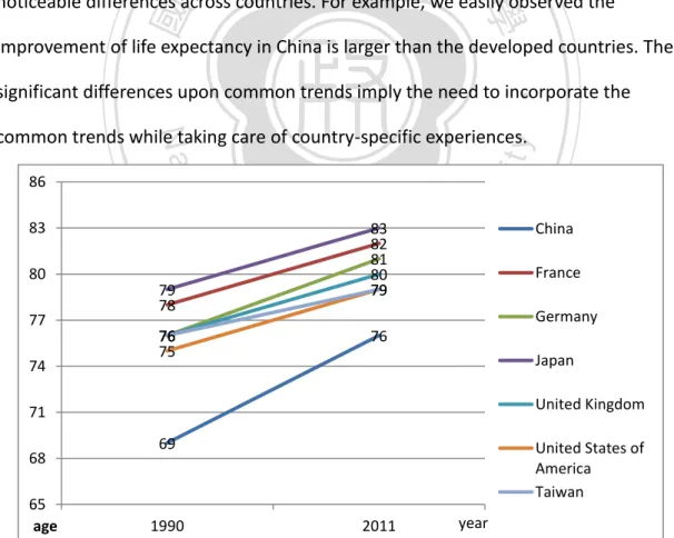
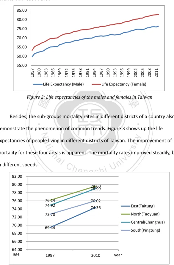
(7) Introduction. For governments and life insurance companies, mortality rates are one of the key factors in determining premiums and reserves. Ignoring or miscalculating mortality rates might have negative influences in pricing. It might also impair the profitability and solvency for governments and insurance companies. In recent years, the mortality improvement is obvious. Figure 1, which based on the statistics report of WHO and authorities concerned, demonstrated the. 政治大 increasing in the past two decades. On the other hand, the increases exhibit 立. improvement were significantly. The life expectancy in several major countries kept. ‧ 國. 學. noticeable differences across countries. For example, we easily observed the improvement of life expectancy in China is larger than the developed countries. The. ‧. significant differences upon common trends imply the need to incorporate the. 77 74. y. sit. n. 83 80. al. er. io. 86. Nat. common trends while taking care of country-specific experiences.. 79 78. Ch. 83 82 81 80 79. engchi. i Un. v. 65 age. France Germany. 76 75. 76 Japan United Kingdom. 71 68. China. 69. United States of America Taiwan. 1990. 2011. year. Figure 1: mortality Improvements of several major countries – population. The common trend of mortality improvement is also founded between groups of a country. Figure 2, which showed up the mortality structures for the male-female 1.

(8) groups of Taiwan, is a good instance. The life expectancies of the males and females in Taiwan increased steadily in the past half a century, but the expectancies are distinct from each other. 85.00 80.00 75.00 70.00 65.00 60.00 2011. 治政大 (Female) Life Expectancy (Male) Life Expectancy 立. 2008. 2005. 2002. 1999. 1996. 1993. 1990. 1987. 1984. 1981. 1978. 1975. 1972. 1969. 1966. 1963. 1960. 1957. 55.00. ‧ 國. 學. Figure 2: Life expectancies of the males and females in Taiwan. ‧. Besides, the sub-groups mortality rates in different districts of a country also demonstrate the phenomenon of common trends. Figure 3 shows up the life. y. Nat. io. sit. expectancies of people living in different districts of Taiwan. The improvement of. n. al. er. mortality for these four areas is apparent. The mortality rates improved steadily, but in different speeds. 82.00 80.00. 74.00 72.00 70.00. engchi. i Un. v. 79.60 78.99. 78.00 76.00. Ch. 76.14 74.92. 76.02 East(Taitung). 74.36. North(Taoyuan). 72.70. Central(Changhua) 69.44. South(Pingtung). 68.00 66.00 64.00 age. 1997. 2010. year. Figure 3: Life expectancies of the people living in different regions of Taiwan 2.

(9) As we mentioned before, for governments and life insurance companies, mortality rates are one of the key factors in determining premiums and reserves. However, most of the models in use did not consider the difference and the relationship between each subgroup. Li and Lee (2005) provided an extension of the Lee-Carter Model which considered the coherent effect for group of populations. This augmented common factor model considered the common trend effect between two subgroups. Based on the coherent Lee-Carter Model, Li and Hardy (2012) compared independent Lee-Carter Method and Augmented Lee-Carter method to estimate the basis risk in longevity hedges. Besides using Lee-Carter. 治政 Models or other extension of Lee Carter Methods, Yang, 大Yue, and Huang (2010) used 立 principal component analysis (PCA) method to capture and forecast the mortality ‧ 國. 學. rate improvement. In their model, they considered the age shifts in mortality. sit. y. Nat. up a 2-PC model to forecast 6 countries life expectancies.. ‧. reductions to capture the variant morality improvement at different ages by setting. io. er. In this article, we will use the mortality data of Taiwan from the human mortality database to build up a multi-group common factors mortality model. We. al. n. iv n C plan to compare the fitting effect ofhour model with independent Lee-Carter Model engchi U and The Augmented Common Factor Lee-Carter Model. We also calculate the premium and reserves of particular policies by different mortality assumption. Our model building may also provide another round of comparisons on the performance of different multi-population models. The remainder of this article is organized as follows: In the section “Literature Reviews and Methodology,” we first introduce some relative articles and recently researches. Our method used in this article will also be mentioned here. In the section “Fitting and Forecasting Results,” we show the results by using different mortality models assumptions. We will compute the premium and reserves by 3.

(10) different assumptions and comparing the differences between methods. In the final section, we give our conclusions and suggestions.. Literature Reviews and Methodology. Lots of scholars have constructed various dynamic mortality models to forecast mortality rates. Lee and Carter (1992) built up a forecasting model for the central death rate as below: ln(𝑚𝑥,𝑡 ) = 𝛼𝑥 + 𝛽𝑥 𝑘𝑡 + 𝜀𝑥,𝑡. (1). 政治大. Where 𝑚𝑥,𝑡 denotes the central death rate in different years, the parameter. 立. 𝛼𝑥 describes the average age-specific mortality, 𝑘𝑡 means the time-varying index. ‧ 國. 學. which captures the overall speed of mortality improvement, 𝛽𝑥 denotes the age-specific parameter, and 𝜀𝑥,𝑡 is assumed be white noise for this model (Lee,. ‧. 2000).. y. Nat. io. sit. There are some extensions of Lee-Carter Model, such as Renshaw and. n. al. er. Haberman (2006), who modified Lee-Carter Model by considering cohort effect, and. Ch. i Un. v. Hyndman and Ullah (2007) identified more common factors. From the basis of. engchi. Lee-Carter Model, Cairns, Blake and Dowd (2006) established another time-series models by using specific functional forms. To consider influence of common trend/factor, Li and Lee (2005) constructed The Augmented Common Factor Lee-Carter Model to capture the common factor between the U.S female and Canada female’s population mortality rate. The Augmented Lee-Carter method is modeled as: ln(𝑚(𝑥,𝑡,𝑖) ) = 𝛼(𝑥,𝑖) + 𝐵(𝑥)𝐾(𝑡) + 𝛽(𝑥,𝑖) 𝑘(𝑡,𝑖) + 𝜀(𝑥,𝑡,𝑖). (2). Where 𝛼(𝑥,𝑖) is describes the average age-specific mortality of each population. The Parameters 𝐵(𝑥) and 𝐾(𝑡) capture the central tendencies within the group of 4.

(11) populations. The parameter 𝛽(𝑥,𝑖) and 𝑘(𝑡,𝑖) , which means the population-specific factor, can be obtained from the residual matrix of the common factor model. Besides Lee-Carter Model and its extensions, some scholars constructed forecasting model by principal component analysis (PCA). The PCA method was invented by Pearson (1901), and Hotelling (1933) developed this model to prove the key factors influence on the school entrance exam is the language and math ability. By PCA method, we can describe the variation in a set of multivariate data in terms of a set of uncorrelated variables. We also often use PCA method to reduce the factors.. 治政 Bell (1997) adopted PCA method with 2-PCs to forecast 大 the U.S. male and 立 female mortality rates, and this 2-PCs model performed better than Lee-Carter ‧ 國. 學. Model. Yang, Yue, and Huang (2010) also adopted PCA method to forecast the. ‧. mortality rate improvement of six countries by setting up a 2-PC model. Njenga and. sit. y. Nat. Sherris (2009) considered the common trend between countries. They first adopted. io. er. PCA method to forecast 5 countries’ population life expectancies. After fitting mortality rates by PCA, they introduced Vector-Autoregressive (VAR) model to find. al. n. iv n C the common trend, and capture long relationships in a Vector h erunnequilibrium gchi U. Error-Correction Model (VECM) framework, which means they use the same loading metrics for every country. The major applications of mortality models are computing the policy premium and reserves, checking out the credit or basis risk for specific insurance companies, and helping government authorities planning social security policies. Li and Hardy (2012) used The Augmented Lee-Carter Model (Li and Lee, 2005) to measure basis risk in longevity hedges. In this article, we improve the PCA method to forecast the life expectancies. We use the sub-groups data to find common PCs. The model we set up as below: 5.

(12) 𝑚𝑥,𝑡 = 𝑙𝑥,1 𝑆1,𝑡 + 𝑙𝑥,2 𝑆2,𝑡 + ⋯ + 𝑙𝑥,𝐾 𝑆𝐾,𝑡. (3). Where 𝑚𝑥,𝑡 means the age-specific mortality rate, 𝑙𝑥,𝑘 denotes the loading of mortality date, and 𝑆𝐾,𝑡 represents the score, which changes with time. When we estimate the future score 𝑆𝐾,𝑡 changes, we use the autoregressive moving average (ARMA) model. The ARMA model combines AR Model and MA model to explain the relationship between variables. The AR model is modeled like: 𝑋𝑡 = 𝐶 + ∑𝑝𝑖=1 𝜑𝑖 𝑋𝑡−𝑖 + 𝜀𝑡. (4). Where p means the log-time, and 𝜀𝑡 denotes the error term. The MA model is modeled like:. 治政 𝑋 =𝜇 +𝜀 +∑ 𝜃 𝜀 (5) 大立 To combine the AR model and MA model, we can rewrite and obtain the ARMA 𝑡. 𝑡. 𝑞 𝑖=1 𝑖 𝑡−𝑖. ‧ 國. 學. model as below:. 𝑡. ‧. 𝑋𝑡 = 𝜇𝑡 + ∑𝑝𝑖=1 𝜑𝑖 𝑋𝑡−𝑖 + ∑𝑞𝑗=1 𝜃𝑖 𝜀𝑡−𝑗. (6). sit. y. Nat. In the Lee-Carter Model and its extensions, 𝑘(𝑡,𝑖) is often estimated by. io. er. autoregressive integrated moving average (ARIMA) model. This model is similar to ARMA model, but it considers the integrated effect. ARIMA is modeled like:. al. iv 𝑝 𝑞 n C 𝑋𝑡 = 𝜇𝑡 + ∑𝑖=1 𝑖 𝜀𝑡−𝑗 h 𝜑e𝑖 𝑋n𝑡−𝑖g+c∑h𝑗=1i 𝜃U n. ∆. 𝑑. (7). In the data selection, we adopt the life expectancies data of Taiwan from 1970 to 2000 from the human mortality database, and estimate future score 𝑆𝐾,𝑡 by using ARMA model. We also follow Lee and Carter (1992) Model and The Augmented Lee-Carter Model (Li and Hardy, 2012) and use the same sample years to fit the actual data of different gender’s life expectancies in Taiwan.. 6.

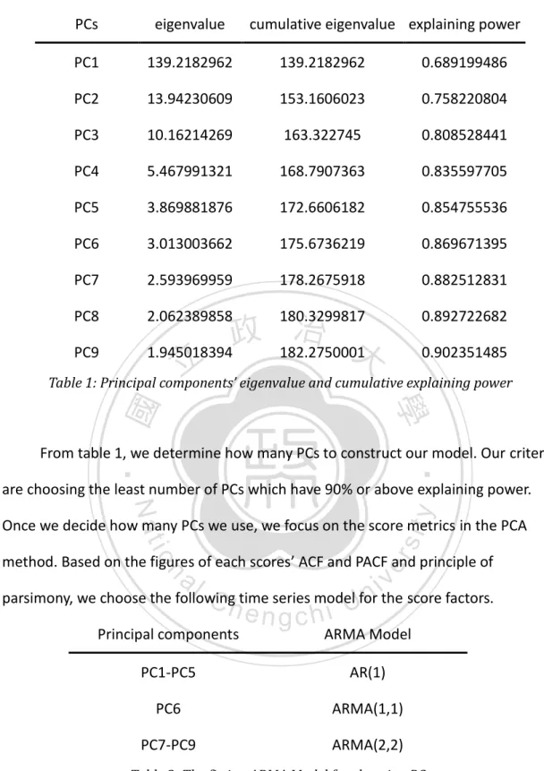
(13) PCs. eigenvalue. cumulative eigenvalue explaining power. PC1. 139.2182962. 139.2182962. 0.689199486. PC2. 13.94230609. 153.1606023. 0.758220804. PC3. 10.16214269. 163.322745. 0.808528441. PC4. 5.467991321. 168.7907363. 0.835597705. PC5. 3.869881876. 172.6606182. 0.854755536. PC6. 3.013003662. 175.6736219. 0.869671395. PC7. 2.593969959. 178.2675918. 0.882512831. PC8. 2.062389858. 180.3299817. 0.892722682 治政 182.2750001大 0.902351485 PC9 1.945018394 立 Table 1: Principal components’ eigenvalue and cumulative explaining power. ‧ 國. 學 ‧. From table 1, we determine how many PCs to construct our model. Our criteria are choosing the least number of PCs which have 90% or above explaining power.. y. Nat. er. io. sit. Once we decide how many PCs we use, we focus on the score metrics in the PCA method. Based on the figures of each scores’ ACF and PACF and principle of. n. al. Ch. i Un. v. parsimony, we choose the following time series model for the score factors. Principal components. engchi. ARMA Model. PC1-PC5. AR(1). PC6. ARMA(1,1). PC7-PC9. ARMA(2,2). Table 2: The fitting ARMA Model for choosing PCs. To compare with other mortality forecasting model, we choose the Lee-Carter Model (Lee and Carter, 1992) and the augmented Lee-Carter Model.( Li and Hardy, 2012). In the Lee-Carter Model and its extensions, we all assume the parameters 𝑘𝑡 , 7.

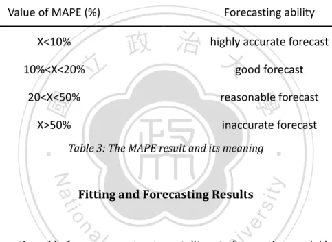
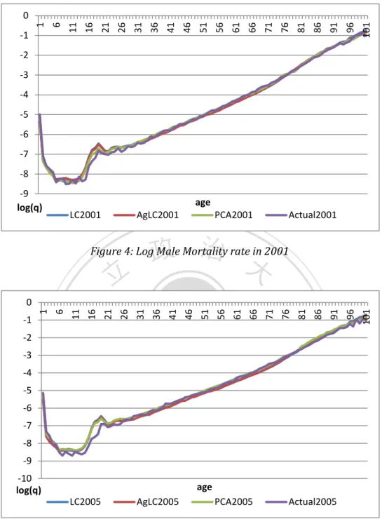
(14) 𝐾(𝑡), and 𝑘(𝑡,𝑖) follow the ARIMA model (0, 1, 0). And to measure the fitting effect, we adopt the Mean Absolute Percent Error (MAPE). As its name, MAPE can help us to compare the forecast ability by using forecasting value and actual value. The MAPE can be obtained by following formula: MAPE =. 1 n. At −Ft. ∑nt=1 |. At. | × 100%. (8). Where 𝐴𝑡 means the actual value, and 𝐹𝑡 means the forecasting value. Lewis (1982) provided the criteria for using MAPE as table 3. Value of MAPE (%) X<10% 10%<X<20%. 立. Forecasting ability accurate forecast 政治 highly 大good forecast reasonable forecast. X>50%. inaccurate forecast. Nat. n. al. er. io. sit. Fitting and Forecasting Results. y. Table 3: The MAPE result and its meaning. ‧. ‧ 國. 學. 20<X<50%. Ch. i Un. v. As mentioned before, we construct mortality rate forecasting model by using. engchi. PCA method. Also, we compare the fitting effect between our model, the Lee-Carter model, and the augmented common factor model. Figure 4 to figure6 are the log male mortality rates for these 3 models with actual mortality rate to compare the fitting ability.. 8.

(15) 96. 101. 96. 101. 91. 86. 81. 76. 71. 66. 61. 56. 51. 46. 41. 36. 31. 26. 21. 16. -1. 11. 6. 1. 0. -2 -3 -4 -5 -6 -7 -8 -9 log(q). age LC2001. AgLC2001. PCA2001. Actual2001. 政治大. -6. -9 -10 log(q). 91. 86. 81. 76. 71. 66. 61. 56. 51. 46. 41. 31. 26. 21. y. al. n. -8. io. -7. Nat. -5. sit. -4. ‧. -3. er. -2. 6. 1 -1. 學. 0. ‧ 國 11 16. 立. 36. Figure 4: Log Male Mortality rate in 2001. Ch. engchi. i Un. v. age. LC2005. AgLC2005. PCA2005. Actual2005. Figure 5: Log Male Mortality rate in 2005. 9.

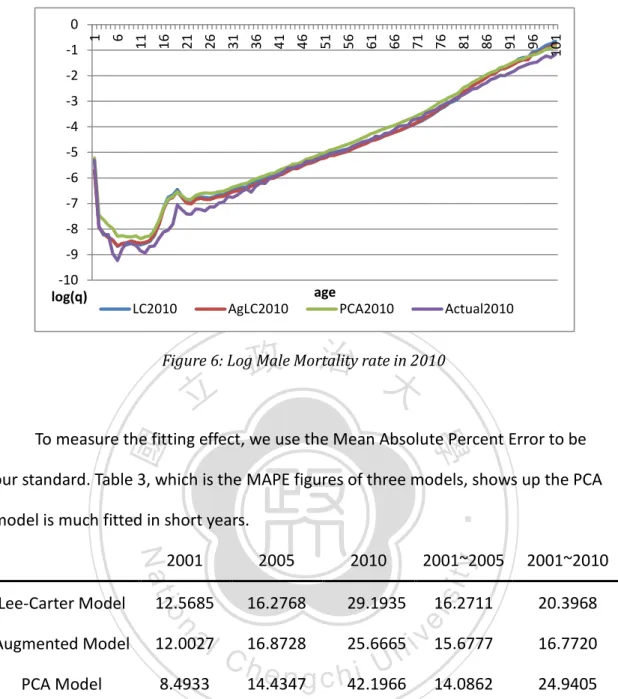
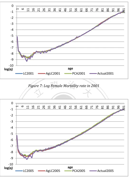
(16) 101. 96. 91. 86. 81. 76. 71. 66. 61. 56. 51. 46. 41. 36. 31. 26. 21. 16. -1. 11. 6. 1. 0 -2 -3 -4 -5 -6 -7 -8 -9 -10 log(q). age LC2010. AgLC2010. PCA2010. Actual2010. 政治大. Figure 6: Log Male Mortality rate in 2010. 立. ‧ 國. 學. To measure the fitting effect, we use the Mean Absolute Percent Error to be our standard. Table 3, which is the MAPE figures of three models, shows up the PCA. ‧. model is much fitted in short years.. 29.1935. 16.8728. n. al. 12.0027. PCA Model. 8.4933. Ch. 2001~2005. y. 16.2768. Augmented Model. 2010. 2001~2010. sit. 12.5685. io. 2005. 16.2711. 20.3968. 25.6665. v 15.6777. 16.7720. i e n g c h42.1966. 14.0862. 24.9405. 14.4347. er. Nat. Lee-Carter Model. 2001. i Un. Table 4: The MAPE of 3 models in forecasting male life expectancies. Again, in figure 7 to figure9, we show these models log mortality rate to compare the fitting and forecasting condition with actual mortality rate.. 10.

(17) 26 31 36 41 46 51 56 61 66 71 76 81 86 91 96 101. 21. 16. -1. 11. 1 6. 0 -2 -3 -4 -5 -6 -7 -8 -9 -10 log(q) LC2001. age PCA2001. AgLC2001. Actual2001. 政治大. -6. -9 -10 log(q). LC2005. y. Ch. engchi. i Un. age PCA2005. AgLC2005. v. Actual2005. Figure 8: Log Female Mortality rate in 2005. 11. 101. 96. 91. 86. 81. 76. 71. 66. 61. 56. 51. 46. 41. 36. 26. 21. al. n. -8. io. -7. Nat. -5. sit. -4. ‧. -3. er. -2. 16. 1 -1. 學. 0. 6 ‧ 國 11. 立. 31. Figure 7: Log Female Mortality rate in 2001.

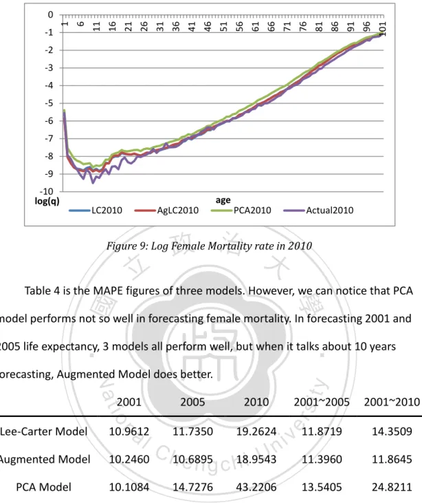
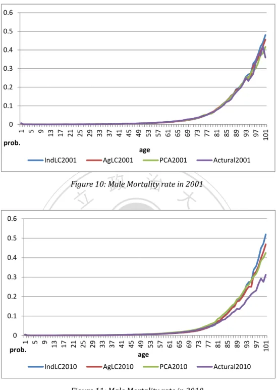
(18) 101. 96. 91. 86. 81. 76. 71. 66. 61. 56. 51. 46. 41. 36. 31. 26. 21. 16. -1. 11. 6. 1. 0 -2 -3 -4 -5 -6 -7 -8 -9 -10 log(q). age LC2010. AgLC2010. PCA2010. Actual2010. 政治大. Figure 9: Log Female Mortality rate in 2010. 立. ‧ 國. 學. Table 4 is the MAPE figures of three models. However, we can notice that PCA model performs not so well in forecasting female mortality. In forecasting 2001 and. ‧. 2005 life expectancy, 3 models all perform well, but when it talks about 10 years. io. al. 10.9612. Augmented Model. 10.2460. PCA Model. 10.1084. n. Lee-Carter Model. y. sit. 2001. 2005. 2010. 2001~2005. 11.7350. 19.2624. v 11.8719 i n. C h10.6895 18.9543 engchi U 14.7276. 2001~2010. er. Nat. forecasting, Augmented Model does better.. 43.2206. 14.3509. 11.3960. 11.8645. 13.5405. 24.8211. Table 5: The MAPE of 3 models in forecasting female life expectancies. As we can see, all three models underestimate the mortality improvement, especially for long-term forecasting. Figure 10 and figure 11, based on the forecasting mortality rate of male, is a good example helps us to capture this phenomenon. From these figures, we notice that all the models extremely overestimate the death rate in the old-age group.. 12.

(19) 0.6 0.5 0.4 0.3 0.2 0.1. 1 5 9 13 17 21 25 29 33 37 41 45 49 53 57 61 65 69 73 77 81 85 89 93 97 101. 0 prob.. age IndLC2001. AgLC2001. PCA2001. Actural2001. 政治大. Figure 10: Male Mortality rate in 2001. 立 0.5 0.4. sit. io. al. n. 0.1. er. 0.2. y. Nat. 0.3. ‧. ‧ 國. 學. 0.6. Ch. engchi. i Un. v. 1 5 9 13 17 21 25 29 33 37 41 45 49 53 57 61 65 69 73 77 81 85 89 93 97 101. 0 prob.. age. IndLC2010. AgLC2010. PCA2010. Actural2010. Figure 11: Male Mortality rate in 2010. However, all of the models have great forecasting power in 5 years, no matter which gender. It can help us construct a 5-year and 10-year projection by using all the year data (from 1970 to 2010). We adopt all method mentioned before, and we obtain the forecasting figure as below.. 13.

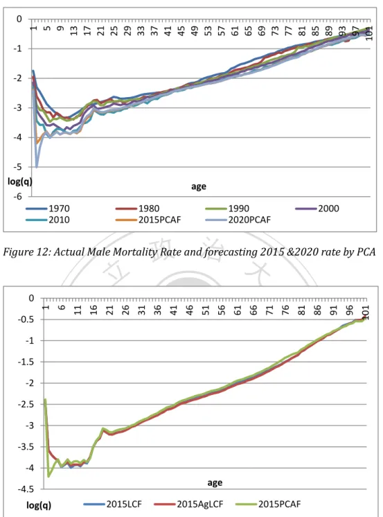
(20) 1 5 9 13 17 21 25 29 33 37 41 45 49 53 57 61 65 69 73 77 81 85 89 93 97 101. 0 -1 -2 -3 -4 -5 log(q) -6. age 1970 2010. 1980 2015PCAF. 1990 2020PCAF. 2000. 政治大. -4. 101. 96. 91. 81. 71. 66. 61. 56. y. sit. Ch. engchi. i Un. v. age. -4.5 log(q). 51. 46. 41. 36. 31. 26. 16. 6. 21. al. n. -3.5. io. -3. er. -2.5. Nat. -2. ‧. -1.5. ‧ 國11. 1 -1. 學. -0.5. 76. 立 0. 86. Figure 12: Actual Male Mortality Rate and forecasting 2015 &2020 rate by PCA. 2015LCF. 2015AgLCF. 2015PCAF. Figure 13: Forecasting 2015 Male Mortality Rates by three models. From these figures, we find out the PCA model performs not so well in the infant-age and mostly overestimate the death rate. All three models have good estimations in the middle-age. It is important for some insurance policies, such as mortgage life insurance, which has lots of middle-aged policyholders.. 14.

(21) 101. 96. 91. 86. 81. 76. 71. 66. 61. 56. 51. 46. 41. 36. 31. 26. 21. 16. 11. 6. 1. 0 -1 -2 -3 -4 -5 age. -6 2020LCF. log(q). 2020AgLCF. 2020PCAF. 政治大. Figure 14: Forecasting 2020 Male Mortality Rates by three models. 立. ‧ 國. 學. As we can see, the PCA method estimates the mortality rate should be higher. Following figures are the estimations for female.. 1 5 9 13 17 21 25 29 33 37 41 45 49 53 57 61 65 69 73 77 81 85 89 93 97 101. ‧. 0. sit. n. al. er. io. -2. y. Nat. -1. -3 -4. Ch. engchi. -5 log(q) -6. i Un. v. age 1970 2010. 1980 2015PCAF. 1990 2020PCAF. 2000. Figure 15: Actual Female Mortality Rate and forecasting 2015 &2020 rate by PCA. 15.

(22) 101. 96. 91. 86. 81. 76. 71. 66. 61. 56. 51. 46. 41. 36. 31. 26. 21. 16. -0.5. 11. 6. 1. 0. -1 -1.5 -2 -2.5 -3 -3.5 -4 -4.5 age. -5 2015LCF. log(q). 2015AgLCF. 2015PCAF. 政治大. -5. Ch. -6 log(q). 101. 96. 91. 86. 81. sit. n. al. er. io. -4. y. Nat. -3. 76. 71. 66. 61. 56. 51. 46. 41. 31. 26. 21. ‧. -2. 6. 1 -1. 學. 0. 11 ‧ 國 16. 立. 36. Figure 16: Forecasting 2015 Female Mortality Rates by three models. 2020LCF. e n gagec h i 2020AgLCF. i Un. v. 2020PCAF. Figure 17: Forecasting 2020 Female Mortality Rates by three models. The major problem for the PCA model in forecasting female mortality is still about the infant-age estimation. Following, we use all of the three models’ forecasting life expectancies to calculate the policy premium and reserve by different scenario. Firstly, we calculate 20 year term-life insurance. All of the mortality assumptions are following the 16.

(23) forecasting 2014 mortality rate by each model, and we fix the discount rate at 1.875%, which is the rediscount rate of Taiwan Central Bank. Also, we set up the policy holder is 30 years old in 2014. We obtain the level premium and FPT reserves of this policy as below: 0.012 0.01 0.008 0.006 0.004. 立. ‧ 國. 0. 4. year. 10 11 12 13 14 15 16 17 18 19 20 21 LC FPT Reserve 2012 TSO FPT Reserve. y. Nat. 5 6 7 8 9 PCA FPT Reserve AgLC FPT Reserve. ‧. 1 2 3 amount per dollar. 學. 0.002. 政治大. n. al. er. io. sit. Figure 18: Comparing reserves by different mortality models with term - male. 0.004 0.0035. Ch. engchi. i Un. v. 0.003 0.0025 0.002 0.0015 0.001 0.0005 0 1. 2. amount per dollar. 3. 4. 5 6 7 8 9 PCA FPT Reserve AgLC FPT Reserve. year 10 11 12 13 14 15 16 17 18 19 20 21 LC FPT Reserve 2012 TSO FPT Reserve. Figure 19: Comparing reserves by different mortality models with term – female. 17.

(24) Natural Premium – 1yr. Level Premium – 2yr after. PCA Forecasting. 0.001269898. 0.00299941. LC Forecasting. 0.001261005. 0.002895322. Augmented LC Forecasting. 0.00118594. 0.002632707. 2012 5th TSO. 0.001041918. 0.002347291. Table 6: The level Premium of 20 year term life insurance - Male. PCA Forecasting LC Forecasting. 立. Augmented LC Forecasting. Level Premium – 2yr after. 0.000429192. 0.000962405. 治 0.00040431 政大. 0.000874664. 0.000425059 0.000394346. ‧ 國. 0.000951229. 學. 2012 5th TSO. Natural Premium – 1yr. 0.00085929. Table 7: The level Premium of 20 year term life insurance - Female. ‧ sit. y. Nat. In the above case, using PCA method will enhance the level premium, and the. n. al. er. io. life insurance companies have to prepare more reserves. In the comparison, using 5th. i Un. v. TSO will lead the life insurance company lower their level premium. One of the. Ch. engchi. possible reason is the 5th TSO is a kind of experienced life table, which considers the underwriting power of life insurance company. In other word, Lee-Carter model with its extensions and PCA method may have accurate forecast if we can obtain the company-specific data. Besides calculating the term-life insurance case, we also demonstrate whole life insurance as another example. As mentioned before, all of the mortality assumptions are following the forecasting 2014 mortality rate by each model and other conditions unchanged. The level premium and FPT reserves of this policy as below: 18.

(25) 0.7 0.6 0.5 0.4 0.3 0.2 0.1 year. 0 1 2 3 amount per dollar. 4. 政治大. 5 6 7 8 9 10 11 12 13 14 15 16 17 18 19 20 21 22 PCA FTP Reserve LC FPT Reserve AgLC FPT Reserve 2012 TSO FPT Reserve. 立. Figure 20: Comparing reserves by different mortality models with whole life - male. ‧ 國 n. al. er. io. sit. y. Nat. 0.4. ‧. 0.5. 學. 0.6. 0.3 0.2. Ch. engchi. i Un. v. 0.1 year 0 1 2 3 4 amount per dollar. 5. 6 7 8 9 10 11 12 13 14 15 16 17 18 19 20 21 PCA FPT Reserve LC FPT Reserve AgLC FPT Reserve 2012 TSO FPT Reserve. Figure 21: Comparing reserves by different mortality models with whole life - female. 19.

(26) Natural Premium – 1yr. Level Premium – 2yr after. PCA Forecasting. 0.001269898. 0.027488934. LC Forecasting. 0.00118511. 0.027481468. Augmented LC Forecasting. 0.00118594. 0.026662906. 2012 5th TSO. 0.001041918. 0.026956194. Table 8: The level Premium of whole life insurance - Male. PCA Forecasting LC Forecasting. 立. Level Premium – 2yr after. 0.000429192. 治政 0.00040431 大. 0.024111376. 0.000425059. 0.023808547. 2012 5th TSO. 0.023711895. 學. ‧ 國. Augmented LC Forecasting. Natural Premium – 1yr. 0.000394. 0.02380314. Table 9: The level Premium of whole life insurance - female. ‧ y. Nat. io. sit. From figures and tables mention above, we still easily notice that all the three. n. al. er. models may overestimate the death rate, and the companies need to keep much. Ch. i Un. v. more reserves. Also, each models’ level premium has huge differences since the. engchi. forecasting mortality rates are quite different. Because of computing FPT reserves, we need to obtain the first year natural premium. This is the reason why the first year’s premiums are same in the 20 year term-life insurance and whole life insurance.. Conclusions and Suggestions. From above analysis, we find out to consider common trend or the common factors helps us to construct the mortality rate model more accurate. No matter we 20.

(27) use the augmented Lee-Carter model or the PCA method, both of them perform well then original independent Lee-Carter model. By using the data of Taiwan population in 1970 to 2000, our common PCA model has the least figure in MAPE in the estimation in 2001 to 2005. If considering the gender difference, our model estimates the male life expectancy more accurate. By setting up PCA method, we can use the forecasting mortality to compute the premiums and reserves for life insurance companies. In previous paragraph, we have also shown the different amount of reserves by different mortality assumptions. However, all of the three models we used in this article overestimate the death. 治政 rate in the future. From the comparison between the actual 大 data of life expectancies 立 and the forecasting figure of these three models, all of them can’t catch the ‧ 國. 學. significant mortality improvement in the infant-age and elder-age. Also, since we. ‧. don’t have enough information to use company-specific data, all of the models. y. sit. io. er. 5th TSO life table.. Nat. overpriced if we compare the level premium with the figure computed by using 2012. One of the solutions is to forecast the future mortality in short period, or. al. n. iv n C capture more components when adopting model. But when we decide to h e n gthecPCA hi U use more parameters, the advantages of reducing parameters will be sacrificed. Another solution is to obtain company-specific data to construct unique models. The following research will focus on the each component’s explaining power and using this method to compare actual loss with company-specific data. From previous figures, we have noticed that all of the three models fit well in middle-age. For the sake of this reason, it is suitable to use this model for mortgage life insurance. Also, since PCA method reflects the time-related shock by only few periods, we can consider the long-term memory effect in our model to improve the forecasting ability. 21.

(28) References. 1. BELL, William R. Comparing and assessing time series methods for forecasting age-specific fertility and mortality rates. JOURNAL OF OFFICIAL STATISTICS-STOCKHOLM-, 1997, 13: 279-304.. 2. Cairns, A. J. G., D. Blake, and K. Dowd, 2006a, A Two-Factor Model for Stochastic Mortality with Parameter Uncertainty: Theory and Calibration, Journal of Risk and Insurance, 73: 687-718.. 3. Dahl, M., 2004, Stochastic Mortality in Life Insurance: Market Reserves and Mortality-linked Insurance Contracts, Insurance: Mathematics and Economics, 35: 113-136.. 立. 政治大. Dahl, M., and T. Møller, 2005, Valuation and Hedging of Life Insurance Liabilities with Systematic Mortality Risk, In the Proceedings of the 2005 International AFIR Colloquium, Zurich, Available online at http://www.afir2005.ch.. 5. Hyndman, R. J. and S. Ullah, 2007, Robust Forecasting of Mortality and Fertility Rates: A Functional Data Approach, Computational Statistics and Data Analysis, 51, 4942-4956.. 6. JARNER, Søren Fiig; KRYGER, Esben Masotti. Modelling adult mortality in small populations: The SAINT model. Astin Bulletin, 2011, 41.02: 377-418.. ‧. ‧ 國. 學. 4. n. er. io. sit. y. Nat. 7. al. Ch. engchi. i Un. v. RENSHAW, Arthur E.; HABERMAN, Steven. A cohort-based extension to the Lee– Carter model for mortality reduction factors. Insurance: Mathematics and Economics, 2006, 38.3: 556-570.. 8. Stallard, E., 2006, Demographic Issues in Longevity Risk Analysis, Journal of Risk and Insurance, 73: 575-609.. 9. LI, Nan; LEE, Ronald. Coherent mortality forecasts for a group of populations: An extension of the Lee-Carter method. Demography, 2005, 42.3: 575-594.. 10 Lee, R. D. and L. R. Carter, 1992, Modeling and Forecasting U.S. Mortality, Journal of the American Statistical Association, 87: 659-675. 22.

(29) 11 Lee, R. D. and T. Miller, 2001, Evaluating the Performance of the Lee-Carter Mortality Forecasts, Demography, 38: 537-549. 12 Li, J. S. H., & Hardy, M. R, 2011, Measuring basis risk in longevity hedges. North American Actuarial Journal, 15(2), 177-200. 13 LEWIS, Colin David. Industrial and business forecasting methods: A practical guide to exponential smoothing and curve fitting. London: Butterworth Scientific, 1982. 14 McNown, R. and A. Rogers, 1989, Forecasting Mortality: A Parameterized Time Series Approach, Demography, 26: 645-660 15 Plat, R., 2009, On Stochastic Mortality Modeling, Insurance: Mathematics and Economics, 45, 393-404.. 立. 政治大. ‧. ‧ 國. 學. 16 Murray, C. J. L., B. D. Ferguson, A. D. Lopez, M. Guillot, J. A. Salomon, and O. Ahmad, 2003, Modified Logit Life Table System: Principles, Empirical Validation, and Application, Population Studies, 57: 165-182.. al. er. io. sit. y. Nat. 17 SHERRIS, Michael; NJENGA, Carolyn. Longevity Risk and the Econometric Analysis of Mortality Trends and Volatility. UNSW Australian School of Business Research Paper, 2009, 2009ACTL08.. v. n. 18 YANG, Sharon S.; YUE, Jack C.; HUANG, Hong-Chih. Modeling longevity risks using a principal component approach: A comparison with existing stochastic mortality models. Insurance: Mathematics and Economics, 2010, 46.1: 254-270.. Ch. engchi. i Un. 19 Yue, C. S. J., & Huang, H. C., 2011. A Study of Incidence Experience for Taiwan Life Insurance. The Geneva Papers on Risk and Insurance-Issues and Practice, 36(4), 718-733.. 23.

(30)