Electrical Interaction Energy between Two Charged Entities in an Electrolyte Solution

FEATURE ARTICLE

Electrical Interaction Energy between Two Charged Entities

in an Electrolyte Solution

Jyh-Ping Hsu1 and Bo-Tau Liu

Department of Chemical Engineering, National Taiwan University, Taipei, Taiwan 10617, Republic of China Received April 5, 1999; accepted May 28, 1999

The electrical interaction energy between two charged entities in an electrolyte solution plays a significant role in various phenom-ena in colloid and interface science. Available methods for the estimation of this energy under the Debye–Huckel condition are discussed briefly, and a systematic approach based on a boundary integral method, which has the potential to yield an approximate analytical expression for various types of surfaces under a general surface condition, is introduced. The linear sizes of the interacting entities can be comparable or one is much larger than the other. A typical example for the former includes, for instance, the interac-tion between two colloidal particles. The stability behavior of a colloidal dispersion belongs to this category. That for the latter includes the interaction between a particle and a wall. The ad-sorption of particles to surfaces and the electrophoretic motion of particles near a boundary, for example, belong to this category. Extensions to more complicated cases, for example, multiple par-ticles and arbitrary surfaces, are also discussed. © 1999 Academic Press Key Words: charged entities; electrical interaction energy;

boundary integral method; Poisson–Boltzmann equation; Debye– Huckel condition.

1. INTRODUCTION

Particulate and interfacial sciences and technologies are foundations to modern chemical process industrials includ-ing such diverse areas as fertilizers, foods, minerals, mate-rials, and energy. Indeed, a majority of the value added by the modern industry is directly related to them. An across-the-board assessment also reveals that they will play the key role in high-tech industries, for example, electronics, ad-vanced materials, biotechnology, and environment, to name a few, of the coming century. A detailed understanding of the mechanisms and phenomena involved is essential not only to the development of new technologies but also to fundamental studies. Often, evaluation of the electrical in-teraction energy between two charged entities needs to be estimated in the description of the relevant analyses. The

broad spectrum of particulate science and interfacial sci-ences includes various possible combinations of solid, liq-uid, and gas phases. In the discussion below, we will focus only on the case in which solid entities are dispersed in a liquid phase containing electrolytes. Although the problem under consideration is classic and has been investigated extensively in the literature most of the discussions are limited to specific geometry or boundary conditions. A systematic approach has not been introduced.

On the basis of the relative magnitudes of the interacting entities, two types of problem can be identified: the sizes of the two interacting entities are comparable, and one of two inter-acting entities is orders of magnitude larger than the other. The coagulation phenomenon of a colloidal suspension in water and wastewater treatment, for example, belongs to the former. Here, the stability behavior of the dispersed system is of main concern. The classic analysis (DLVO theory) for an aqueous dispersion of lyophobic colloidal particles involves the calcu-lation of the electrical and van der Waals interactions between two charged particles (1). The goal here is to seek conditions, which lead to an unstable system; that is, the attractive force between two particles overcomes the repulsive force between them, and coagulation between particles occurs. In some other cases, searching for conditions which yield a stable dispersion becomes the key issue. For instance, how to maintain the stability of the slurry used in chemical–mechanical polishing (2, 3) is essential to a wafer production process. The attach-ment of particles to surfaces is one of the typical examples in which the sizes of two interacting entities are orders of mag-nitude different. It is also possible that a problem involves both types of interactions. The electrophoretic motion of a particle in which either the effect of nearby particles or the presence of a boundary needs to be considered is one of the typical exam-ples in practice.

Recent advances in direct force measurement techniques based on surface force apparatus (4, 5) allow an accurate estimation of the forces between charged particles and sur-faces. Apparently, quantitatively identifying the electrical force is essential to the estimation of various other possible interac-1_{To whom correspondence should be addressed.}

219 0021-9797/99 $30.00

Copyright © 1999 by Academic Press All rights of reproduction in any form reserved.

tion forces, e.g., hydration force, steric force, and van der Waals force, involved when two entities approach each other. The purpose of this work is to summarize briefly the available methods in the literature for the evaluation of the electrical interaction energy between two charged entities and to intro-duce a systematic approach based on a boundary integral method. The latter is capable of leading to an approximate analytical result for problems often encountered in practice. We will limit the discussion to a low to medium level of electrical potential mainly for two reasons. First, estimating the interaction energy analytically for an arbitrary level of electri-cal potential can be done only for extremely limited cases, and a numerical scheme is required for most of the problems. Second, if the electrical potential is high, there is a lack of rigorous governing equation for the description of its spatial variation. The discussion ends with a brief description of the problems that are of both practical and theoretical significance and deserve further study in the near future.

2. BASIC EQUATIONS

The estimation of the electrical interaction energy between two charged entities comprises two steps in a series: determine the spatial variation in the electrical potential, and conduct an integration over a specified domain which simulates a charging process.

2.1. Electrical Potential

At equilibrium, assuming that the distributions of electrolyte ions in the liquid phase follow the Boltzmann distribution, the spatial variation of electrical potential of the system under consideration can be described approximately by the so-called Poisson–Boltzmann equation. This equation needs to be solved subject to the boundary conditions reflecting the nature of the charged entities and the domain considered.

2.1.1. Poisson–Boltzmann Equation

Suppose that the electrolyte ions can be treated as point charges. Then the ionic flux of ion species i, Ni, comprises the contribution due to concentration gradient and that due to electrical field, called the Nernst–Planck relation:

Ni5 2Di

S

¹ni1 ZiF

RT ni¹c

D

. [1]

Here ¹ denotes the gradient operator; F and R are, respec-tively, the Faraday constant and the gas constant; Di, Zi, and

ni, are, respectively, the diffusivity, the valence, and the con-centration of ion species i; and c is the electrical potential. Applying the condition that ions are unable to penetrate the surface of a rigid entity, Eq. [1] leads to

ni5 ni`exp

S

2 ZiFc

RT

D

, [2]

where ni`is the bulk value of ni. That is, the spatial variation of ions follows the Boltzmann distribution. Suppose that the permittivity of the liquid phase,e, is constant. Then the rela-tionship between electrical potential and space charge density r is

2_{c 5 2}r

e, [3]

where 2 denotes the Laplace operator. The space charge density can be expressed as

r 5

O

i

niZiF, [4]

where the summation is over all the charged species in the liquid phase. Substituting Eqs. [2] and [4] into Eq. [3] gives

2c 5 2F

e

O

_i Zini`exp

S

2

ZiFc

RT

D

. [5]

This is the Poisson–Boltzmann equation. Although its statisti-cal mechanistatisti-cal grounds have been questioned, the performance of Eq. [5] in describing the diffuse double layer near a charged surface in an electrolyte solution is found to be satisfactory (6).

For symmetric Z:Z electrolytes, Eq. [5] becomes 2

y5k2

sinh y, [6]

where the scaled potential y is defined by y5 ZFc/RT, and k2 _{5 2F}2

Z2

C/eRT, k being the reciprocal Debye length.

Gouy and Chapman (1, 6) were able to derive an analytic solution of Eq. [6] for an infinite planar surface. For other geometries and unsymmetric electrolytes, solving Eq. [5] an-alytically becomes difficult. Hsu and Liu (7) were able to derive a perturbation solution for a spheroidal surface in a symmetric electrolyte solution, and Hsu and Kuo (8) obtained a semi-analytical result for cylinderical and spherical surfaces. If the electrical potential is sufficiently low, Eq. [5] can be approximated by

2c 5 k2c,

[7] the so-called Debye–Huckel approximation. The linear nature of this expression makes it easier to be solved than Eq. [6]. Unfortunately, if more than one charged surface is present, exactly solvable cases are still very limited.

2.1.2. Boundary Conditions

Various types of surface conditions are possible in practice. We will consider three cases, which are assumed mostly in the relevant analyses.

2.1.2.1. Constant potential/charge surfaces. Suppose that

the electrical potential on an entity surface remains constant, that is,

c 5 cS, [8]

wherecSdenotes the surface potential, which can be position dependent. If the surface charges arise from a surface reaction, or the exchange of potential determining ions with the bulk liquid phase, then assuming a constant surface potential is equivalent to assuming that the rate of surface reaction or that of exchanging of potential determining ions occurs infinitely fast. Equation [8] is a Dirichlet-type condition.

If the charge density on the entity surface si is fixed, we have

s 5 si. [9]

Compared with the case of constant surface potential, this is equivalent to assuming that the rate of surface reaction or that of exchanging of potential determining ions occurs infinitely slow. Note that if the permittivity of the solid phase is much smaller that of the liquid phase, then applying the Gauss divergence theorem leads to, at entity surface, s 5 2e(­c/ ­n). Therefore, Eq. [9] can be viewed as a Neumann-type condition.

2.1.2.2. Charge-regulated surfaces. Under certain

cir-cumstances the surface of an entity is capable of regulating its charged condition as a response to the variation in the nearby environment. A typical example includes surfaces of an am-photeric nature such as biological surfaces (9 –17). Let us consider the case where the following surface reactions occur:

AB2

Z1_{7 AB1 B}Z1 _[10a]

AB 7 AZ2_{1 B}Z1_{. [10b]}

In these expressions, AB denotes the functional group, and BZ1 is the potential determining ion, Z being its valence. For amphoteric surfaces, BZ1

is usually the hydrogen ion (6). Let

K1 and K2, be the dissociation constants of Eqs. [10a] and [10b], respectively. The net surface charge density can be evaluated by (11) s 5 s0 d sinh@~cN2cS!/c0# 11d cosh@~cN2cS!/c0# , [11] wheres0 5 eZNS, c0 5 RT/F, cN 5 2.303(pK0 2 pB)c0, pK0 5 (pK1 1 pK2)/ 2, DpK 5 pK22 pK1, andd 5 2 3 102DpK/ 2. In these expressions, NSand T are the number density of the functional group and the absolute temperature, respec-tively,cNis the Nernst potential, which is related to the point of zero charge when pK0 5 pB. A surface with a low DpK is

capable of regulating its charged condition efficiently so that its surface potential is more or less constant as the separation distance between two surfaces varies (18). In contrast, a sur-face with a highDpK is considered to have properties close to those with a constant surface charge.

Note that ifcS is low, Eq. [11] can be approximated by

s 5 s0 d sinh~cN/c0! 11d cosh~cN/c0! 2 d cos~cN/c0! 1d 2 @1 1d cosh~cN/c0!# 2 s0 c0c S 5 J 2 GcS [12] with J 5s0 d sinh~cN/c0! 11d cosh~cN/c0! [12a] G 5 d cosh~cN/c0! 1d2 @1 1d cosh~cN/c0!#2 s0 c0 . [12b]

Equation [12] indicates that the boundary condition is of mixed nature. Note that the constant surface potential and constant charge density conditions, represented by Eqs. [8] and [9], respectively, can be recovered as the special cases of Eq. [12].

2.1.2.3. Charged membranes. Another important class of

charged entities is that which has a porous or ion-penetrable, charged surface layer. Typical example includes biological cells, e.g., blood cells and protein aggregates (19 –24), and entities covered by an artificial membrane, e.g., particles with an adsorbed polymer layer and porous entities (25, 26). These particles are characterized by having its fixed charges distrib-uted over a finite volume in space, rather than over a rigid surface. In this case, an additional source term needs to be added to the right-hand side of Eq. [5] for a point inside membrane to reflect the presence of fixed charges, i.e.,

2_{c 5 2}F e

O

_i Zini`exp

S

2 ZiFc RT

D

2 rf e , [13]

whererf denotes the density of fixed charges.

2.2. Electrical Interaction Energy

If the surfaces of two rigid entities remain at constant po-tential, the electrical interaction energy, Vel, can be evaluated

Vel5 2

ES

E

0

cS

Ds~c9S!dc9SdS, [14]

where Ds 5 s 2 siso, s and siso being, respectively, the

surface charge density of a particle when both particles are present and that of an isolated particle. If the surface potential is low, Eq. [14] becomes

Vel5 2

1 2

E

S

DscSdS. [14a]

If two particles remain at constant surface charge density, then

Vel5

ES

E

0

s

DcS~s9!ds9dS, [15]

whereDcS 5 cS 2ciso,cisobeing the surface potential of an

isolated particle. IfcS is low, Eq. [15] becomes

Vel5

1

2

ES

sDcSdS. [15a]

For two charge-regulated hard spheres, Carnie and Chan (27) were able to derive the following expression:

Vel5

ES

F

E

0 s DcS d_{~s9!ds9 2}

E

0 s DcS S_~s9!ds9

G

dS. [16] Here, DcS S 5 cS S 2 ciso S , ciso S

being the value of cS S

for an isolated particle, is the relation between surface potential and surface charge density that has to be satisfied as a result of surface reactions such as Eq. [10], and the functionDcS

d 5 cS d 2 ciso d ,ciso d

being the value ofcS d

for an isolated particle, the surface potential calculate according to the Poisson–Boltzmann equation. For low electrical potentials, Eq. [16] becomes, after applying Eqs. [7] and [12],

Vel5

1

2J

E

S

DcSdS. [17]

For an ion-penetrable membrane which is capable of regu-lating its charged conditions, an expression which is similar to the case of a hard sphere with a charge-regulated surface can be written Vel5

EV

F

E

0 si DcS d_~s9 i!ds9i2

E

0 si DcS S_~s9 i!ds9i

G

dV, [18]

where V is the volume of membrane phase. For low electrical potentials, Eq. [18] becomes, after applying Eqs. [7] and [12],

Vel5

1

2J

E

V

DcSdV. [19]

As presented in the Appendix, the electrical interaction energy can also be evaluated based on Maxwell stress and osmotic pressure (28).

3. SOLUTION METHODS

Evaluation of the electrical interaction energy between two charged entities is nontrivial, in general, even for simple ge-ometry at low electrical potentials. An analytical expression can be obtained only for very limited cases. McCormack et al. (29), for example, derived the electrical double-layer force and interaction free energy between two planar surfaces of various surface conditions in a symmetric electrolyte solution. In prac-tice the interaction energy is evaluated either by a direct numerical integration or by an approximate analytical method. The latter, although not exact, is capable of providing a simple expression, which is highly desirable for subsequent analysis. In statistical mechanics, the difficulty of estimating the elec-trical interaction energy between two charged entities is often circumvented either by assuming a primitive model (30 –32) or by assuming that it has the Yukawa form (33). The latter is based on the assumption that the double layer near a charged surface is thick and/or the separation between two entities is large (34, 35). Other approaches include that proposed by Derjaguin and Landau (36) and linear superposition. The latter is appropriate if the distance between two charged entities is longer than the Debye length; if this is not the case, the former becomes appropriate. Several attempts have been made in the past two decades to improve the performance of Derjaguin approximation (37– 41). However, since the entity– entity dis-tance can be in the medium range, a more satisfactory proce-dure is desirable for practical considerations. To this end, a systematic approach, which is applicable to a general charged condition, was proposed recently (42). A brief discussion about the available methods is given below.

3.1. Numerical Methods

Numerical methods provide a powerful and direct way of obtaining the solution of a problem, which is difficult to solve analytically. It avoids complicated mathematical treatments, and the result obtained is usually accurate. The finite difference method, which discretizes the computational domain into a

finite number of intervals (43– 45), for example, is a useful tool for problems defined over a simple domain. If a global coor-dinate is difficult to be defined, e.g., two arbitrarily oriented spheroids, the finite element method, which discretizes the computational domain into a finite number of elements, can be applied. Problems using this method include, for example, two identical spheres (46), a cylinder and a plane (47), a biomac-romolecule (48), a short cylinder (49), and a sphere and a charged pore (50). Due the degree of precision specified, however, numerical methods may face the convergence prob-lem, and developing an efficient algorithm is essential. Also, parametric study can be tedious, and in view of the possible mathematical treatments in the subsequent analyses, a numer-ical solution is not as attractive as an analytnumer-ical expression.

3.2. Approximate Analytical Methods

Several methods, which lead to approximate analytical re-sults, are introduced briefly.

3.2.1. Derjaguin and Modified Derjaguin Approximations

Derjaguin (51) suggested that if two spheres are sufficiently close to each other, the interaction energy between them can be estimated based on that of two planar parallel surfaces. This method is appropriate if the closest surface-to-surface distance between two entities is on the order of Debye length. One of the popular applications based on Derjaguin’s approximation is that proposed by Hogg et al. (52) for two rigid spheres; the result obtained is found to be accurate for thin double layers. Several attempts were made to improve the performance of Derjaguin’s approximation for thicker double layers. Often, the solution of a Poisson–Boltzmann equation is estimated either by expanding the electrical potential based on the result of Gouy and Chapman, i.e., the solution for two parallel, planar surfaces, or through an iterative procedure based on that. Although these methods lead to better results the improvement in the degree of accuracy is limited, and sometimes the proce-dure involved can be tedious. Derjaguin’s approximation can be modified to improve its performance for a moderate level of electrical potential (53, 54). It was also incorporated with another method (55).

3.2.2. Multipole Expansion

This approach is based on the assumption that the solution to a Poisson–Boltzmann equation can be expanded in a series of harmonic functions Rn

c 5

O

n

CnRn. [20]

The coefficient Cn is determined by the associated boundary conditions based on the orthogonal property of Rn (56 –59). The electrical potential obtained is then used to evaluate the

interaction energy. The approach is semi-analytic, and its per-formance depends largely on the choice of harmonic functions and the number of terms used. It should be pointed out that choosing Rnadequately can be nontrivial for irregular surfaces. Also, if a mixed boundary condition such as Eq. [12] is assumed, then the orthogonal property of Rnbecomes invalid. In this case Cn needs to be evaluated through solving a large set of simultaneous algebraic equations (60).

3.2.3. Boundary Collocation Method

This method is similar to multipole expansion. It is assumed that the solution to Eq. [7] can be approximated by a linear combination of a finite number of harmonic functions, i.e., the upper limit of n in Eq. [20] is a finite number M. After substituting the assumed solution into Eq. [7], sufficiently many points on the domain boundary are chosen so that coef-ficient Cn, n 5 1, 2, . . . , M, can be determined. A set of linear algebraic equations needs to be solved. As in multipole expansion, choosing an appropriate set of harmonic functions can be nontrivial for irregular surfaces. Also, its performance is usually unsatisfactory if the level of surface potential is high. Another problem is the choice of M. Often, a considerable amount of computing time is necessary to reach a convergent solution.

3.2.4. Boundary Integral and Boundary Element Methods

The boundary integral method is based on the fact that the solution of Eq. [7] can be expressed as an integral of its Green function over the boundary of problem domain. In other words, the dimensionality of the original problem can be reduced by one through adopting this approach. The boundary conditions are incorporated automatically into the integral representation of the solution of Eq. [7]. For irregular surfaces evaluating directly the integral is difficult, and it is approximated by a system of algebraic equations obtained through discretizing the boundary, the so-called boundary element method. The bound-ary integral method has the merit that it has the potential of obtaining an analytical solution. This, however, is often non-trivial even for regular surfaces. The boundary element method, in contrast, has the merit that it is more readily applicable to irregular surfaces. However, the results obtained are numerical, and developing an efficient algorithm can be time consuming.

3.2.5. Reflection Method

Let us label the entities in a system as entities 1 and 2. Ifc(0)

denotes the potential due to the presence of isolated entity 1, then it will not satisfy the condition on the surface of entity 2. This is compensated for by adding a correction termc(1)

toc(0)

. But now the corrected potential may not satisfy the condition on the surface of entity 1. Therefore the potential is further corrected by adding a new termc(2)

until the resultant potential satisfies the specified surface con-ditions. The final solution takes the form

c 5 c~0!_1c~1!_1c~2!_{1 · · ·. [21]}

In principle, an analytic expression can be obtained. It, how-ever, is usually complicated (58, 61– 63), and the rate of convergence can be a problem.

3.2.6. Linear Superposition

Linear superposition assumes that the result of multiple charged entities can be approximated by a linear combination of the results for individual entities. For instance, ifc1andc2

are the solutions of Eq. [7] for isolated entities 1 and 2, respectively, then the solution of Eq. [7] when both entities are present is approximated by

c 5 c11c2. [22]

Analyses which applied this approach include, for example, two plates covered with charge-regulated layers (64), two spheres covered by an ion-penetrable membrane (16), and two spheroids (65). Although it is simple and straightforward, linear superposition is limited to the case when the distance between two entities is longer than two Debye lengths. Another possible case in which linear superposition is applicable is ion-penetrable entities. An image-interaction correction strat-egy was proposed by Ohshima (66) to improve the perfor-mance of linear superposition for the case of two dissimilar spheres. Similar to the case of the reflection method, however, the result obtained is complicated.

4. A SYSTEMATIC APPROACH BASED ON BOUNDARY INTEGRAL

In a recent study, Hsu and Liu (42) applied the boundary integral method to various types of entity– entity interactions. An approximate analytical expression for the electrical inter-action energy between two charged entities can be derived through a systematic approach. Their approach is introduced in the following discussion. Let us consider two charged entities with boundaries S1 and S2, respectively, in an electrolyte

solution. It can be shown by direct substitution that a particular solution to Eq. [7] is

G~r! 5exp~2kr!

4pr , [23]

where r is the scaled position vector from a fixed point charge, and G is the free Green function (67). Applying Green’s first identity, the solution to Eq. [7] can be expressed as

c 5

O

i51 2

E

Si

F

G e si1cSixi

G

dS, [24] where xi5 ­G ­ni , i5 1, 2. [24a]

In these expressions, ni is the normal vector of Si toward the liquid phase, and cSi and si are, respectively, the surface potential and the surface charge density of entity i. The dielec-tric constant of the entities is assumed to be much smaller than that of the liquid phase. It can be shown that, for a point on Sj, we have (68) 1 2cSj5

O

i51 2

E

Si

F

G e si1cSixi

G

dSi. [25]

Consider the general linear boundary condition represented by Eq. [12],

si5 Ji2 GicSi, [26]

whereJiandGi are constant. If bothJiandGi are large, Eq. [26] yields a constant potential condition withcSi5 Ji/Gi. If Gi3 0, then the surface charge of Siremains constant atsi5 Ji. Other than these cases, Si can be regarded as a charge-regulated surface (10, 11, 14).

Substituting Eq. [26] into Eq. [25], we obtain

1 2cSj5

O

i51 2

E

Si

H

Ji e G1

S

2Gi e G1xi

D

cSi

J

dSi. [27]

Suppose thatcSi can be decomposed as cSi5cSi

0 _{1 Dc}

Si, [28]

wherecSi

0

is the unperturbed surface potential of isolated entity

i, andDcSiis a perturbed surface potential of entity i due to the presence of the other entity. Suppose that cSi

0 is position-independent. Then cSi 0 ₅ Ji e bii 1 21 Gi e bii2gii , [29]

where bii5

E

Si GiidSi [29a] gii5

E

Si xiidSi [29b]

In these expressions Giiandxiiare, respectively, the values of

G andxiwhen both of the two end points of the position vector are on Si. Suppose that the electrical potential for isolated entity i can be expressed as

ci5cSi

0_u

i, [30]

where ui is a function of the position in the liquid phase. Substituting Eqs. [28]–[30] into Eq. [27], we obtain

1 2DcS15

ES

1

S

2G1 e G1x1

D

DcS1dS1 1

ES

2

S

2G2 e G1x2

D

DcS2dS21cS2 0_u 12 [31a] 1 2DcS25

ES

1

S

2G1 e G1x1

D

DcS1dS1 1

E

S2

S

2G2 e G1x2

D

DcS2dS21cS1 0_u 21, [31b]

whereuji is the value ofui when one of the end points of the position vector is on Sj. Equations [31a] and [31b] are implicit expressions for DcSj, which have the form of an integral equation with an inseparable kernel, and, therefore, solving them directly is difficult. This difficulty can be circumvented by replacing approximately Eqs. [31a] and [31b] by a set of algebraic equations, which are readily solvable. The procedure is based on the fact that the surface integral of a smooth function Z can be approximated by

E

ZdS>

O

i51 M

wiZi, [32]

where wiis a weighting factor, and Ziis the value of Z at point

i. The values of wi and M depend on the integration scheme

adopted. On the basis of Eq. [32] Eqs. [31a] and [31b] can be expressed as xDc 5 B, [33] where Dc 5 @Dc1,1,Dc1,2,. . .Dc1,M,Dc2,1, . . . ,Dc2,M#t [33a] : 5

F

:1,1 :1,2 :2,1 :2,2

G

[33b] :l,k5 @:i, j,l,k#, i, j 5 1, . . . , M, l, k 5 1, 2 [33c] :i, j,l,k5 2wj

S

2Gk e Gk, j l,i _1x k, j l,i

D

, i, j5 1, . . . , M, l, k5 1, 2, i Þ j or l Þ k 51₂2 wj

S

2Gk e Gk, j l,i _1x k, j l,i

D

, i5 j and l 5 k, i, j5 1, . . . , M, l, k 5 1, 2 [33d] B5

3

cS2 0 u12,1 z z cS2 0_u 12,M cS1 0_u 21,1 z z cS1 0_u 21,M

4

. [33e]

In these expressions, superscript t represents matrix transpose,

Gk, j l,i

andxk, j l,i

are, respectively, the values of G andx in which the distance r is measured from point j of entity k to point i of entity l, and the differentiation is conducted on Sk,uji,kdenotes the values ofuji evaluated at point k of entity j. If l 5 k and

i 5 j, then Gk, j l,i

and xk, j l,i

become singular. In this case the following approach is applicable. Equations [29a] and [29b] suggest that Gk, jk, j

andxk, j k, j

can be evaluated by subtracting the contribution of all other Gk, jl,i

and xk, j l,i

from Gkk and gkk, respectively, that is,

:j, j,k,k5 1 22

S

2Gk e bkk1gkk

D

1

O

i51 iÞj M wi

S

2Gk e Gk,i k, j_1x k,i k, j

D

. [34] For the present linear system the electrical interaction energy between two entities can be calculated by employing Eq. [17]

Vel5 1 2J1

E

S1 DcS1dS1 1 2J2

E

S2 DcS2dS. [35]

SinceDcSiusually varies smoothly over Si, the dimensions of the matrices in Eq. [33] need not be large, and it can be solved efficiently. Substituting the solution of Eq. [33] into Eq. [35], the electrical interaction energy between two entities can be calculated.

4.1. Approximate Analytical Expression

Obtaining an approximate analytic form for DcSj is also possible by adopting the method proposed by McCartney et al. (69) and Bell et al. (28). According to Eqs. [23] and [24a], both

G and xi become very large when a singular point is

ap-proached. This suggests thatDcSi on the right-hand sides of Eqs. [31a] and [31b] can be moved out from the integral sign, and we have

S

1 22g111 G1 e b11

D

DcS11

S

G2 e b122g12

D

DcS25cS2 0_u 12 [36a]

S

G1 e b212g21

D

DcS11

S

1 22g221 G2 e b22

D

DcS25cS1 0_u 21, [36b] where bji5

E

Si GjidS [36c] gji5

E

Si xjidS. [36d]

Here Gjiandxji are respectively the values of G andxiwhen one of the end points of the position vector is on Si and the other on Sj, jÞ i. The relationship amongbii,bji,gii, andgji will be discussed later. For the time being, we claim that

bji5biiuji [37a]

gji5

S

1

21gii

D

uji. [37b]

It should be pointed out that Eq. [37b] is applicable only if the condition that, ifsi is uniform, then the corresponding cSi

0

is also uniform, is satisfied. Equation [37a], however, does not have this limitation.

Solving Eqs. [36a] and [36b] for DcSj, j 5 1, 2, and substituting the resultant expressions into Eq. [35], we obtain

Vel 1₅ e 2b11

ES

1 cS1 0_c S2 0 _{1 f} 2cS1 0 2_u 21 12 f1f2u12u21 u 12dS [38a] Vel 2₅ e 2b22

E

S2 cS1 0_c S2 0 _{1 f} 1cS2 0 2_u 12 12 f1f2u12u21 u 21dS, [38b] where f15 1 21g112 G11 e b11 1 22g111 G11 e b11 [38c] f25 1 21g222 G22 e b22 1 22g221 G22 e b22 . [38d]

Employing the approximate procedure adopted by Sader et al. (53), Eqs. [38a] and [38b] can be rewritten, respectively, as

Vel 1₅ e 2b11

E

S1

F

cS1 0_c S2 0 _{1 f} 2cS1 0 2_u 12 12 f1f2u12 2

G

u12dS [39a] and Vel 2₅ e 2b22

E

S2

F

cS1 0_c S2 0 _{1 f} 1cS2 0 2_u 21 12 f1f2u21 2

G

u21dS. [39b]

4.2. Some Useful Relations

Referring to Fig. 1a, Siis a simple closed surface, its interior and exterior are denoted byVi

andV0

, respectively. Let r be the distance between two points. rii represents the value of r when both of these points are on Si, and rrirepresents the value of r when one of the two points is on Siand the other point not on Si. Referring to Fig. 1a, rri

i

is the value of rriwhen one of its two points is on Siand the other point inVi

, and rri0

is that of rriwhen one of its two points is on Siand the other point in V0

. Also, Gii and Gri become the values of G(r) when r is replaced by rii and rri, respectively, andbji andgji needed to be replaced bybri andgri, respectively. Since directly evalu-atingbii,bri, gii, and gri can be nontrivial we suggest using the procedure below.

Step 1. Determinebiiandbri. Let S1 be an infinitely thin

electrical potential inside the shell, ci

, and that outside the shell,c0 , can be expressed as ci₅c S1ui [40a] c0_5c S1u 0 , [40b]

where cS1 is the surface potential, u i

is a function of the position in Vi, and u0 is a function of the position in V0. According to the Green’s function theory (67), the spatial variation of electrical potential and the surface potential can be expressed, respectively, as c 5s1 e bri [41] and cS15 s1 e bii [42] Therefore, bii5 ecS1 s1 . [43]

IfcS1ands1are known, thenbiican be determined. It should be emphasized that Eq. [41] is valid if the distribution of surface charge is uniform. Equations [40a], [40b], [41], and [43] lead to bri i _5b iiu i [44a] bri 0 _5b iiu 0 , [44b] wherebri i andbri 0

are the values ofbri associated with rri i

and

rri

0

, respectively.

Step 2. Determinegiiandgri. To determinegiiandgri, we consider the two cases shown in Figs. 1b and 1c. The former represents a charged, rigid surface S2with its interior, and the

latter a charged, rigid surface S2 with its exterior. The surface

potential on S2 is denoted as cS2. It can be shown that the

electrical potential inside S2for the case of Fig. 1b,c

i

, and that outside S2 for the case of Fig. 1c, c

0 , can be expressed, respectively, as ci₅c S2ui [45a] and c0_5c S2u 0 . [45b]

Suppose that both the surface potentialcS2and the correspond-ing surface charge densitys2 are position-independent. Then,

according to Green’s function theory,ci and c0 can also be expressed as ci₅s2 e bri i _1c S2gri i [46a] c0₅s2 e bri 0 _1c S2gri 0 [46b] and 1 2cS25 s2 e bii1cS2gii. [46c]

FIG. 1. (a) A simple closed surface S1, with its interiorV

i

and exteriorV0

. r is the distance between two points, riirepresents the value of r when both

of these points are on Si, rri i

is the value of r when one point is on Siand the other inV i

, and rn

0

denotes that of r when one point is on Siand the other in

V0

. (b) A charged, simple closed surface S2with its interiorV

i

. (c) A charged, simple closed surface S2with its exteriorV 0

Therefore we have gii5 1 22 s2 ecS2b ii. [47]

Equations [45a]–[47] yield gri i ₅

S

1 21gii

D

u i [48a] gri 0₅

S

1 21gii

D

u 0 , [48b] wheregri i andgri 0

are the values of gri associated with rri i

and

rri

0

, respectively. Note that, withui andu0

defined in steps 1 and 2, even if S1 5 S2 andcS1 5 cS2,s1 Þ s2, in general.

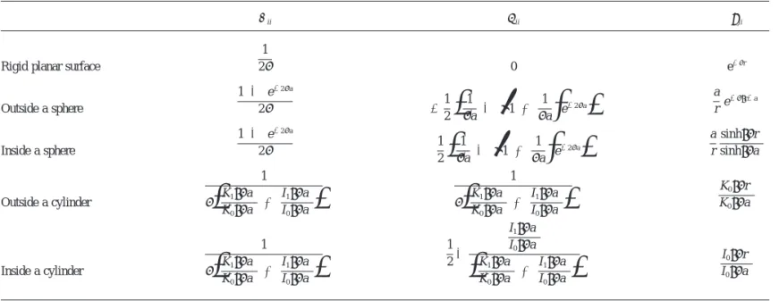
Table 1 summarizes the results forbii, gii, anduji for some typical cases (42).

4.3. Examples

Several examples are illustrated to justify the applicability of Table 1.

4.3.1. Two Spheres

Referring to Fig. 2, we consider two spherical particles in an electrolyte solution. These particles may have different sizes. R is the center-to-center distance between two particles, r21is the

distance between the center of particle 1 and the surface of

particle 2, and a1 and a2 are the radii of particles 1 and 2,

respectively. Applying Table 1, Eqs. [39a] and [39b] can be approximated, respectively, by Vel 1 5pea1a2 b11R

ER

2a2 R1a2 c S1 0_c S2 0 _{1 f} 2cS1 0 2 e2k~r122a2! 12 f1f2e22k~r122a2! 3 e2k~r122a2!_dr 12 [49a] and Vel 2 5pea1a2 b22R

ER

2a1 R1a1 c S1 0_c S2 0 _{1 f} 1cS2 0 2 e2k~r212a1! 12 f1f2e22k~r212a1! e2k~r212a1!_dr 21. [49b] TABLE 1

Results forbii,gii, andujifor Some Typical Geometries (42)

bii gii uji

Rigid planar surface

1 2k 0 e2kr Outside a sphere 1 2 e22ka 2k 21 2

F

1 ka 2

S

1 1 1 ka

D

e22ka

G

a re 2k~r2a! Inside a sphere 1 2 e22ka 2k 1 2

F

1 ka 2

S

1 1 1 ka

D

e22ka

G

a r sinh~kr! sinh~ka! Outside a cylinder 1 k

F

K1~ka! K0~ka! 1 I1~ka! I0~ka!

G

1 k

F

K1~ka! K0~ka! 1 I1~ka! I0~ka!

G

K0~kr! K0~ka! Inside a cylinder 1 k

F

K1~ka! K0~ka! 1 I1~ka! I0~ka!

G

1 22 I1~ka! I0~ka!

F

K1~ka! K0~ka! 1 I1~ka! I0~ka!

G

I0~kr! I0~ka!

Note. r is the distance from a rigid planar surface, that from the center line of a cylindrical surface or that from the center of a spherical surface. a denotes the radius of a sphere or a cylinder. Inand Knare, respectively, the modified Bessel function of the first and the second kind of order n, n5 0, 1.

FIG. 2. Schematic representation of the system under consideration. R is the center-to-center distance between particles 1 and 2, r12 is the scaled

distance between the center of particle 2 to a point on the surface of particle 1, and a1and a2are respectively the scaled radii of particles 1 and 2.

In the derivation of these expressions,uji in the bracket of the right-hand side of Eqs. [39a] and [39b] is approximated re-spectively by exp[2k(r122 a2)] and exp[2k(r212 a1)], as

was done in Sader et al. (53). For thin double layers, the following relations are applicable:

ln~1 1 ab! > b z ln~1 1 a!, a, b 3 0, [50a] tan21~ab! > b z tan21~a!, a, b 3 0. [50b] Summing Eqs. [49a] and [50b], and applying these relations, we obtain Vel5 pea1a2 R

H

f2cS1 0 2_{1 f} 1cS2 0 2 f1f2 ln~1 2 f1f2e22k~R2a12a2!! 14cS1 0_c S2 0

Î

u f1f2u

F

tan21~

Î

u f1f2ue2k~R2a12a2!!, f1f2, 0 tanh21~

Î

f1f2e2k~R2a12a2!!, f1f2. 0

GJ

. [51] The performance of this expression was found to be satisfac-tory, and the higher the ionic strength, the better the perfor-mance (42). For a constant surface potential cSi, Eq. [51] becomes Vel5ep a1a2 R $~cS11cS2! 2 ln~1 1 e2k~R2a12a2!! 1 ~cS12cS2! 2 ln~1 2 e2k~R2a12a2!!%. [52] This is the same as that obtained by Sader et al. (53). For thin double layers, Eq. [51] can further be simplified as

Vel5 4pea1a2cS1 0_c S2 0 e 2k~R2a12a2! R . [53]

This expression can also be derived by neglecting the second term on the left-hand side of Eq. [36a] and the first term on the left-hand side of Eq. [36b] and substituting the resultant ex-pressions into Eq. [35].

4.3.2. A Sphere and a Plane

As illustrated in Fig. 3, we consider a spherical particle (entity 2) of radius a2and a planar surface (entity 1). Let h be

the closest surface-to-surface distance between them, let r21be

the distance between the planar surface and particle surface, and let r12be the distance between the center of the particle and

the planar surface. Applying Table 1, Eqs. [39a] and [39b] can be approximated, respectively, by Vel 1₅pea2 b11

E

n1a2 0 c S1 02_{1 f} 2cS1 0 2 e2k~r122a2! 12 f1f2e22k~r122a2! e2k~r122a2!_dr 12 [54a] Vel 2₅pea2 b22

E

h h12a2 c S1 02 1 f1cS2 0 2 e2kr21 12 f1f2e22kr21 e2kr21_dr 21. [54b]

In the derivation of Eq. [54a],u21 in the bracket of the

right-hand side of Eq. [39a] is approximated by exp[2k(r122 a2)],

as was done in Sader et al. (53). For thin double layers, summing Eq. [54a] and [54b], and applying Eqs. [50a] and [50b], we obtain Vel5pea2

H

f2cS1 0 2_{1 f} 1cS2 0 2 f1f2 ln~1 2 f1f2e22kh! 14cS1 0_c S2 0

Î

u f1f2u

F

tan21~

Î

u f1f2ue2kh!, f1f2, 0 tanh21~

Î

f1f2e2kh!, f1f2. 0

GJ

. [55]

This expression is similar to that derived by Carnie and Chan (27), which was based on Deryaguin’s approximation. It was shown that, regardless of the types of surface condition, the performance of Eq. [55] is satisfactory and is better than that based on Deryaguin’s approximation (42).

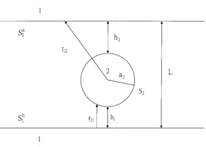
4.3.3. Sphere in a Planar Slit

Referring to Fig. 4, we consider a spherical particle (entity 2) of radius a2in a planar slit S1 (entity 1) of width L. The latter

comprises two surfaces, S1

a and S1

b

. Let h1 and h2 be,

respec-tively, the closest surface-to-surface distance between particle and S1

a

and that between particle and S1

b

, r21 be the distance

from S1to particle surface, S2, and r12be the distance from the

center of the particle to S1. For the present case, since S1is the

union of S1

a and S1

b

, we have

FIG. 3. A spherical particle (entity 2) of radius a2and a planar surface

(entity 1). h is the closest surface-to-surface distance between particle and planar surface, r21the distance from the planar surface to particle surface, and

b115baa 1 _1b ab 1 ₅ 1 2k 1 e2kL 2k 5 11 e2kL 2k [56a] g115gaa 1 _1g ab 1 _{5 0 1}e 2kL 2 5 e2kL 2 . [56b]

It can be shown that for two planar, parallel surfaces with a surface-to-surface distance L,

uji5

e2kr1 e2k~L2r!

11 e2kL . [57]

On the basis of Eqs. [56a], [56b], [57] and Table 1, Eqs. [39a] and [39b] can be approximated, respectively, by

Vel 1₅ ea2 2b11

E

S1 cS1 0_c S2 0 _{1 f} 2cS1 0 2 e2k~r122a2! 12 f1f2e22k~r122a2! e2k~r122a2! r12 dS [58a] and Vel 2₅ e 2b22~1 1 e2kL!

ES

2

F

cS1 0_c S2 0 1 f1cS2 0 2 e2kr21 12 f1f2e22kr21 e2kr21 1cS1 0_c S2 0 1 f1cS2 0 2 e2k~L2r21! 12 f1f2e22k~L2r21! e2k~L2r21!

G

_{dS. [58b]} Summing these expressions, and applying Eqs. [50a] and [50b], we obtain Vel5pea2 11 e2k~h22h1! 11 e2kL

H

f2cS1 0 2_{1 f} 1cS2 0 2 f1f2 ln~1 2 f1f2e22kh1! 14cS1 0 _c S2 0

Î

u f1f2u

F

tan21~

Î

u f1f2ue2kh1!, f1f2, 0 tanh21~

Î

f1f2e2kh1!, f1f2. 0

G

, h2$ h1. [59]

4.3.4. Sphere in a Spherical Pore

Let us consider a spherical particle (entity 2) of radius a2in

a spherical pore (entity 1) of radius a1shown in Fig. 5. Let h

be the closest surface-to-surface distance between the particle and the pore and R be the center-to-center distance between the particle and the pore. r12 and r21 represent, respectively, the

distance between the center of the particle and the surface of the pore and that between the center of the pore and the surface of the particle. Using Table 1, Eqs. [39a] and [39b] can be approximated, respectively, by Vel 1₅ ea2 2b11

E

S1 cS1 0_c S2 0 _{1 f} 2cS1 0 2 e2k~r122a2! 12 f1f2e22k~r122a2! e2k~r122a2! r12 dS [60a] and Vel 2₅ ea1 2b22

E

S2

F

cS1 0_c S2 0 _{1 f} 1cS2 0 2 e2k~r212a1! 12 f1f2e22k~r212a1! e2k~r212a1! r21

G

dS. [60b]

FIG. 5. A spherical particle (entity 2) of radius a2and a spherical pore

(entity 1) of radius a1. h is the closest surface-to-surface distance between

particle and pore, R is the center-to-center distance between particle and pore,

r12and r21denote the distance from the center of the particle to the surface of

the pore and that from the center of the pore to the surface of the particle, respectively.

FIG. 4. A spherical particle (entity 2) of radius a2in a planar slit S1(entity

1) of width L, S1 5 S1

a

ø S1

b

. h1 and h2 are, respectively, the closest

surface-to-surface distance between particle and S1

a

and between particle and

S1

b

, r21is the distance from S1to particle surface, S2, and r12the distance from

For thin double layers, applying Eqs. [50a] and [50b] gives Vel5pea1a2 12 e22kR R

H

f2cS1 0 2_{1 f} 1cS2 0 2 f1f2 ln~1 2 f1f2e22kh1! 14cS1 0_c S2 0

Î

u f1f2u

F

tan21~

Î

u f1f2ue2kh1!, f1f2, 0 tanh21~

Î

f1f2e2kh1!, f1f2. 0

GJ

. [61]

If the centers of the particle and the pore coincide, R5 0, and

VDL can be derived from Eqs. [38a] and [38b]. We have

Vel5 2pe ~1 2 f1f2u12u21!

H

a1 2_u 12 cS1 0_c S2 0 _{1 f} 2cS1 0 2_u 21 b11 1 a2 2_u 21 cS1 0_c S2 0 _{1 f} 1cS2 0 2_u 12 b22

J

. [62]

4.3.5. Sphere Inside/Outside a Cylindrical Pore

Let us consider a spherical particle (entity 2) of radius a2in

a cylindrical pore (entity 1) of radius a1 illustrated in Fig. 6.

Here, h is the closest surface-to-surface distance between the particle and the pore, and r12 and r21 are, respectively, the

distance between the center of the particle and the surface of the pore and that between the axis of the pore and the surface of the particle. Using Table 1, Eqs. [39a] and [39b] can be approximated, respectively, by Vel 1₅ ea2 2b11

E

S1 cS1 0_c S2 0 _{1 f} 2cS1 0 2 e2k~r122a2! 12 f1f2e22k~r122a2! e2k~r122a2! r12 dS1 [63a] and Vel 2₅ ea1 2b22

E

S2

3

cS1 0_c S2 0 _{1 f} 1cS2 0 2I0~kr21! I0~ka1! 12 f1f2

S

I0~kr21! I0~ka1!

D

2 I0~kr21! I0~ka1!

4

dS2. [63b] In the derivation of Eq. [63a],u21 in the bracket of the

right-hand side of [39a] is approximated by exp[2k(r12 2 a2)].

Although obtaining an analytical expression for Vel 1

and Vel 2

becomes difficult in this case, they can be estimated by inte-grating numerically the right-hand sides of Eqs. [63a] and [63b]. In a study of a similar problem where a sphere is placed axisymmetrically in a cylindrical pore, Pujar and Zydney (70) were able to derive an analytical expression for electrical potential and an approximate expression for electrical interac-tion energy. The former is based on a method proposed by Smith and Deen (71) and involves a harmonic expansion, the coefficients of which needed to be determined through a com-plicated procedure. The performance of the present boundary integral method and that of Pujar and Zydney (70) are found to be comparable (42). Note that the derivation of Eqs. [63a] and [63b] does not require axisymmetry.

If the sphere is outside the cylindrical pore, Eqs. [63] and [63b] are still applicable except that the r12 in the former is

now defined as the distance between the center of the sphere and the surface of the cylindrical pore, and r21 and I0 in the

latter are replace by the distance between the axis of the pore and the surface of the sphere, and K0, the modified Bessel

function of the first kind of zero order, respectively.

FIG. 6. A spherical particle (entity 2) of radius a2in a cylindrical pore (entity 1) of radius a1. h is the closest surface-to-surface distance between particle

and pore, and r12and r21the distance measured from the center of the particle to the surface of the pore and that from the axis of the pore to the surface of the

5. MORE COMPLICATED PROBLEMS

The systematic approach introduced in Section 4 can also be applied to various more complicated problems of practical significance. Several examples are illustrated.

5.1. Spheres with a Membrane Layer

Let us consider two spherical particles; each comprises a rigid core and a membrane phase, which contains fixed charges of densityri. In this case, Eqs. [24] and [25] must be modified, respectively, as (72) c 5

O

i51 2

H

ES

i

F

G e si1cSixi

G

dS1 1 e

E

Vi riGdV

J

[64] and 1 2cSj5

O

i51 2

H

ES

i

F

G e si1cSixi

G

dSi1 1 e

EV

i riGdV

J

. [65]

In these expressionscSi andsi are, respectively, the surface potential and surface charge density of the rigid core of particle

i. If the net charge on the rigid core–membrane interface is

zero, si vanishes. Otherwise, the conditions regarding the interface and the membrane phase must be specified. If the distribution of fixed charge in the membrane phase is uniform, thenriis constant, and Eqs. [64] and [65] can be solved. If this is not the case, then solving these equations may become difficult. For instance,rican be a function of electrical poten-tial, which occurs if the degree of dissociation of the functional groups in the membrane phase depends upon electrical poten-tial.

5.2. Multiple Charged Entities

The classic DLVO theory is based on the interaction be-tween two rigid, charged particles, i.e., the concentration of particles is sufficiently low so that the probability of finding three or more particles simultaneously in a small region is negligible. If the concentration of particles is appreciable, either a statistical mechanics approach (73) or a numerical method (74) needs to be employed. Note that information about the interaction between two particles is still required in the former. Hsu and Tseng (60) proposed an iterative proce-dure for the resolution of Eq. [7] for multiple charged, rigid spheres under a general surface condition. The procedure has the merit that a system containing a large number of particles can be simulated by one which has relatively few particles.

Let us consider using the boundary integral method intro-duced in Section 4. For the case of N spheres, Eq. [24] needs to be modified as (75) c 5

O

i51 N

E

Si

F

G e si1cSixi

G

dS, [66] where xi5 ­G ­ni , i5 1, 2, . . . , N [66a] 1 2cSj5

O

i51 N

E

Si

F

G e si1cSixi

G

dSi. [66b]

Also, Eqs. [33a], [33b], and [33e] must be modified, respec-tively, as Dc 5 @Dc1,1, . . . Dc1,M,Dc2,1, . . . , Dc2,M, Dc3,1, . . . ,DcN,M#t [67a] : 5

3

:1,1 z z z :1,N z z z z z z :N,1 z z z :N,N

4

[67b] and B5











O

i52 N cSi 0_u 1i,1 z z

O

i52 N cSi 0_u 1i,M

O

i51 iÞ2 N cSi 0_u 2i,1 z z

O

i51 iÞ2 N cSi 0_u 2i,M z z z

O

i51 N21 cSi 0_u 2i,M











, [67c]

S

1 22gii1 G1 e bii

D

DcSi1

O

i51 jÞi N

S

Gj e bij2gij

D

DcSj 5

O

j51 jÞi N cSj 0_u ij, i5 1, . . . , N. [68]

Note that eachDcSi in this expression is a function. Solving this equation forDcSiand substituting the resultant expression into Eq. [17] the electrical interaction energy can be deter-mined. The results for some special cases can be found in Hsu and Liu (75).

5.3. Arbitrary-Shaped Surfaces

Since charged entities can assume various shapes in practice, a systematic approach, which is readily applicable to surfaces of an arbitrary geometry, is desirable. Hsu and Liu (76) showed that this is possible for ion-penetrable or porous particles. For rigid surfaces, the boundary integral method introduced in Section 4 is applicable if bii, bji, gii, and gji can be deter-mined. However, the results based on Eqs. [29] and [37b] may not be as accurate as those for a simple geometry. In this case, Eq. [37b] needs to be derived, and Eqs. [38a] and [38b] become, respectively, Vel 1 5J1 2

E

S1 3 c2 0

S

1 22g221 G2 e b22

D

1c1

S

g122 G2 e b12

D

S

1 22g111 G1 e b11

DS

1 22g221 G2 e b22

D

2

S

g212 G1 e b21

DS

g122 G2 e b12

D

dS [69a] and Vel 2₅J2 2

E

S2 3 c1 0

S

1 22g111 G1 e b11

D

1c2 0

S

_g 212 G1 e b21

D

S

1 22g111 G1 e b11

DS

1 22g221 G2 e b22

D

2

S

g212 G1 e b21

DS

g122 G2 e b12

D

dS, [69b] whereci 0

is the electrical potential of isolated particle i on the surface of particle j, i Þ j. Nevertheless, it is expected that

Eqs. [29] and [37b] still provide reasonably accurate estimates forcSi

0

andgji, respectively. The rationale behind this is similar to that in the derivation of Eqs. [36a] and [36b] from Eqs. [31a] and [31b]. For an isolated particle j, Eqs. [24] and [25] be-come, respectively, cj5

ES

j

F

G e sj1cSjxj

G

dSj [70] and 1 2 cSj5

E

Sj

F

G e sj1cSjxj

G

dSj. [71]

Since both G andxi become very large if a singular point is approached, as an approximation,sj(orcSj) on the right-hand sides of Eqs. [70] and [71] can be moved out from the integral sign, even ifsj (orcSj) is position-dependent.

5.4. Nonequilibrium Systems

If the surface condition of an entity varies as a response to the variation in the nearby environment, the nonequilibrium behavior of the double layer near the entity should be consid-ered. Charge-regulated surface is one of the typical examples in which the time-dependent nature of the degree of dissocia-tion of the funcdissocia-tional group it bears can be significant. The nonequilibrium behavior of a double layer can also be impor-tant if the distance between two charged entities varies with time. Overbeek (77), for instance, pointed out that the relax-ation time for surface charges is on the order of 1026to 1024s, and the time scale for Brownian coagulation is on the order of 1027 to 1025 s. This implies that the contact between two particles may occur before the electrical condition reaches equilibrium. The effect of the dynamic behavior of the double layer is found to be significant also on various types of entity– entity interactions (78 – 86). At the present stage, methods available for the resolution of problems involving nonequilib-rium electrical interactions between two charged entities are mainly numerical, and developing a systematic approach de-serves further study. If the surface conditions of two entities are functions of time, but the time scale for double-layer relaxation is short, then the systematic approach introduced in Section 4 is applicable.

5.5. Primitive Models

The classic DLVO theory provides a successful theoretic prediction for the coagulation behavior of a colloidal disper-sion, in particular, the Schulze–Hardy rule, which summarizes the experimental observation of the valence dependence of the critical coagulation concentration of counterions. This theory is based on the model of the electrical double layer originating

from the Go¨uy–Chapman theory (87, 88), in which the equi-librium electrical potential is described by Eq. [5]. Here, ions are considered as point charges and the solvent phase a con-tinuum. Equation [5] can be viewed as a mean field approxi-mation for the model used in the Go¨uy–Chapman theory where the correlation between ions is neglected, and ions are different only in their charge. Another basic assumption of the DLVO theory is that the concentration of dispersed particles is low so that the effect of the nearby particles on the interaction of two particles can be neglected. Also, their contribution to the ionic strength is negligible. The basic assumptions of the DLVO theory limit its application in the description of several impor-tant phenomena. For instance, experimental observation re-veals that the critical coagulation concentration of a counterion may vary not only with the valence but also with the size of both the counterion and the coion. In the modeling of the behaviors of liquid– glass transition, polyelectrolyte suspension used in sensor, and solution containing conducting liquid crys-talline polymers, the concentration of a dispersed phase is usually high and considers the interaction between two entities only becomes unrealistic. Another example is the electrical double layer near a metal– oxide surface in an aqueous elec-trolyte solution where water molecules play an important role in the inner Stern layer.

In the past two decades, a steady progress based on statis-tical mechanics in the elaboration of the effect of finite sizes of electrolyte ions on the behaviors of a dispersed phase taking the effect of their concentrations into account is observed. The so-called primitive model is capable of predicting several in-teresting phenomena. For example, the oscillations in spatial variations of both electrical potential and interaction force, and the electrical force between two identical charged surfaces can be attractive (30, 89 –96). The effect of the sizes of the elec-trolyte ions on the behavior of an electrical double layer is found to be significant (97, 98). If the sizes of electrolyte ions are significant, a many-body problem needs to be considered. Often, either a statistical mechanics approach or a Monte Carlo simulation is adopted. The former involves solving the integral equations governing the spatial variation of ion–ion, particle– ion, and particle–particle correlation functions, and developing a numerical scheme is usually necessary. The statistical me-chanics approach is more rigorous than the classic DLVO treatment in the sense that the finite sizes of ions and the concentration of colloidal particles are taken into account. The formulation of a problem, however, is usually complicated and a closure for correlation function needs to be assumed. Often, Coulomb’s law is used to evaluate the interaction force be-tween two charged entities, and spherical geometry is assumed for simplicity. Using this law also requires that the type of boundary conditions assumed need to be simple. These limi-tations can be unrealistic for cases such as polyelectrolytes and colloids with appreciable sizes. In these cases, the boundary integral method introduced in Section 4 is applicable if the free Green function is selected adequately.

6. CONCLUDING REMARKS

Evaluation of the electrical interaction energy between two charged entities in an electrolyte solution is essential to the prediction of many significant phenomena in colloid and in-terface science. For low electrical potentials, boundary integral method has the potential to arrive at an approximate analytical expression for electrical interaction energy under a general surface condition. Also, it is applicable to various types of surfaces and the number of charged entities. Modification of the classic double-layer model to take the finite sizes of elec-trolyte ions into account becomes necessary for various prob-lems which are of both fundamental and practical significance. Developing a systematic approach for the estimation of the interaction energy is challenging in these cases. Revisiting many of the classic problems, for example, coagulation be-tween particles, adsorption of particles to surfaces, and elec-trophoresis, to name a few, based on a primitive model for double layer may lead to unexpected results. Prediction and/or elaboration of the behaviors of biocolloids such as cells and microorganisms also deserve detailed study.

APPENDIX A

The electrical fore between two charged particles can be calculated by (28)

F5

E

G

FS

Dp 1eE

2

2

D

n2e~E z n!E

G

dG, [A1] whereG represents an arbitrary plane between two particles, n is the unit outer normal, and E the electrical field vector with strength E. The osmotic pressure,Dp, can be evaluated by

Dp 5 RT

O

i

ni`

S

exp

S

2 ZiFc

RT

D

2 1

D

. [A2]

For symmetric Z:Z electrolytes Eq. [A2] becomes

Dp 5 e

S

RT_ZF

D

2

k2_{@cosh~ y! 2 1#.}

[A3]

If the electrical potential is low, Eq. [A2] reduces to

Dp 5e₂k2c2

. [A4]

The electrical interaction energy, Vel, between two particles