Physical Design for Reconfigurable Computing System

行政院國家科學委員會專題研究計畫 期中進度報告

子計畫五：可重組化系統之實體設計(2/3)

計畫類別： 整合型計畫

計畫編號： NSC92-2215-E-002-018-

執行期間： 92 年 08 月 01 日至 93 年 07 月 31 日

執行單位： 國立臺灣大學電子工程學研究所

計畫主持人： 張耀文

報告類型： 精簡報告

處理方式： 本計畫可公開查詢

中 華 民 國 93 年 6 月 1 日

多媒體通訊系統中可重組化運算技術之研究

子計畫五：可重組化系統之實體設計(2/3)

Physical Design for Reconfigurable Computing System

計畫編號：NSC 92-2215-E-002-018

執行期限：92 年 8 月 1 日至 93 年 7 月 31 日

計畫主持人：張耀文副教授 國立臺灣大學電子工程學研究所

一

､

中文摘要

動態可重組程式閘陣列(DRFPGAs)被利用來 處理具有高度複雜性和功能的設計，因其可利用時 間共享(time-sharing)方式來增進邏輯效能。在這 篇報告中，我們用 3D-box 表示每一個任務(task) 來處理因為動態可重組程式閘陣列而產生的 3 維平 面規劃和擺置(floorplanning/placement)。我們 提出一個新的以樹狀結構為基礎(tree-based)的 表示法-時序樹(T-tree)。每一個結點(node)至多 有三個子結點來表示任務中空間和時間的關係。我 們提出一個有效的求解方法並導出要滿足任何因 動態可重組程式閘陣列執行而產生的時間順序限 制所需的條件。實驗結果顯示跟現今最頂尖的表示 法相比，我們以樹狀結構為基礎的表示法可以在較 少的時間中得到非常好的解。 關鍵詞：可重組化系統，可重組化計算，實體設計，三 維平面規劃

二､英文摘要(Abstract)

Improving logic capacity by time-sharing, dynamically reconfigurable FPGAs are employed to handle designs of high complexity and functionality. In this report, we model each task as a 3D-box and deal with the temporal floorplanning/placement problem for dynamically reconfigurable FPGA architectures. We present a tree-based formulation, called T-tree, to represent the spatial and temporal relations among tasks. Each node in a T-tree has at most three children which represent the dimensional relationship among tasks. We present an efficient packing method and derive the condition to ensure the satisfaction of precedence constraints which model the temporal ordering among tasks induced by the execution of dynamically reconfigurable FPGAs. Experimental results show that our tree-based formulation can achieve significantly better solution quality with less execution time than the most recent state-of-the-art work.

Keywords: reconfigurable system,

reconfigurable computing, physical design, 3D floorplanning

三､

背景和目的

1. Background

A Field Programmable Gate Array (FPGA) typically consists of regular identical reconfigurable cells (logic blocks) and interconnects around these blocks. Traditionally, an FPGA can only implement circuits by loading the serial configuration bit-streams into the chip at starting time, and the reconfiguration must be done in a whole. Recently, various new architectures have been proposed by various vendors, such as the Atmel AT40K series [1], the Xilinx XC6200 [7] series and the Xilinx Virtex II series [11]. These new-generation FPGAs are partitionable and partially reconfigurable, allowing several tasks and circuits to share the same physical locations at different times and part of the chip to be reconfigured at run-time.

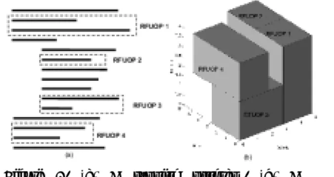
Due to the capability of partially reconfigurable of recent FPGAs, studies have shown that an FPGA-based computation hardware system can improve performance for many applications[7,9]. A reconfigurable system usually consists a host processor and an FPGA coprocessor called reconfigurable function unit (RFU) [2]. During the execution of one program, an RFU may have several configurations at different times. Figure 1(a) shows a program code that can be mapped into four RFU operations (RFUOPs or modules). Since the RFUOP must be placed on the RFU and has its execution time, we may denote each RFUOP as a 3D-box. Because of the area constraint, we cannot load all RFUOPs at the same time. Thus, at time 2, RFUOP 3 is swapped out and RFUOP 4 is swapped in. The question of how to place these RFUOPs becomes a 3D-placement problem. Each module is represented as a 3D-box with the spatial dimensions X and Y and the temporal dimension T. There exist temporal ordering requirements among tasks because one task's input may be another task's output. The goal of temporal floorplanning is to schedule all modules on an RFU so that the specified objective function (e.g., the product of chip area and execution time---the volume of the 3D floorplan/placement) is optimized and no two modules violate the temporal constraints.

Figure 1. (a) A running program. (b) A 3D-placement of the running program.

One significant purpose of a temporal floorplanner is to be a scheduler embedded in the compiler of the host CPU. For some applications, the flow of the program has already been known in advance (for example, in DSP applications). Thus, the scheduler can schedule all RFUOPs that must be executed on the RFU before the program starts. Also, the scheduler can perform various optimizations on the configuration of the RFU, such as the reconfiguration overhead.

四

､

研究方法

We discuss the underlying techniques, approaches, and solutions for handling the proposed problems.

1. Problem formulation for the temporal floorplanning

In the reconfigurable architecture, a task v is loaded into the device for a period of time for execution. Therefore, each task can be represented as a 3D module with spatial dimension x and y and the temporal dimension t. Through this report, we use task and module interchangeably. Let V={v1, v2,...,

vm} be a set of m tasks whose widths, heights, and

execution time are given by Wi, Hi, and Ti, 1 ≦ i ≦

m. We use (xi, yi) ((x'i, y'i)) to denote the coordinate

of the bottom-left (top-right) corner of a task vi and ti

(t'i) the starting (ending) time of task vi, 1 ≦ i ≦ m ,

scheduled in the reconfigurable device. These tasks often need to be executed in a specific order because one task's input could be another task's output. The temporal ordering among tasks is referred to as the precedence constraint in the 3D floorplanning problem. Let D={(vi, vj)|1 ≦ i, j ≦ m, i ≦ j } denote the

precedence constraint for the tasks vi and vj (i.e., vi

must be executed before vj). The precedence

constraints should not be violated during floorplanning/placement.

In order to measure the quality of a floorplan, we consider the same objectives as in [4] and [12]. They are volume, wirelength, communication and reconfiguration overheads.

The definitions of these four objective functions are given below.

Volume (the minimum bounding box of a

placement ): In temporal floorplanning, we

need to consider the area of a device and the

total execution time trade-off. If we use a larger device, the total execution time could be shorten. In contrast, it takes longer time if a smaller one is used. Therefore, we shall minimize the product of the area of the device and the total execution time.

Wirelength (the summation of the half

bounding box of interconnections): Due to the

special architecture of the reconfigurable device, the method to estimate the wirelength in the temporal floorplanning is different from the traditional floorplanning/placement problem. Given a net, those nodes in the net may be executed at the same time or at different times. If they are executed at the same time, we can estimate the wirelength according to their geometric distance directly. However, we have to project all nodes onto the same time frame before computing their wirelength if they are executed at different time frames.

Communication overhead: We quantify the communication overhead based on the Xilinx Virtex XCV1000. Similar to the work by Fekete et al. [4], we assume that a task communicates with another task (data-dependence) in the following way: the results of a CLB, which are read by the successor task, are first written to external memory through a bus interface. The dependent task, which has been loaded at the specified position, then perform a read-in of the results. Recall that a frame is the atomic unit that can be written to or read from. Each frame contains 1248 bits and the bus width is only 8 bit. Thus, it takes approximately 1248/8+24=180 clock cycles in each read-in or read-out, where the 24 cycles are used to configure the bus interface as described on the Xilinx FPGA data book~ [10]}. Therefore, the communication overhead of each reconfiguration takes 360 \times f clock cycles time (we should first write the data to the external memory and then read back the data) if data in f columns need to be transferred.

Reconfiguration overhead: As described in [10], Xilinx Virtex XCV1000 is column-oriented (i.e., all bits in one column should be updated in each read-in or read-out). Suppose that a task vi occupies Wi × Hi CLBs.

We have to reconfigure Hi columns of CLBs in

each reconfiguration. As an example, each CLB column in a Virtex FPGA consists of 48 frames, which takes (1248/8) × 48+24=7512 clock cycles to configure per CLB column. This means we need Wi × 7512 clock cycles in total

if the addresses in the column are incrementally updated.

In this report, we treat a task vi as a

assignment of (xi, yi, ti) for each vi, 1 ≦ i ≦ m ,

such that no two boxes overlap and all precedence constraints are satisfied. The goal of temporal floorplanning is to optimize a predefined cost metric (defined in the above) induced by a placement.

2. Techniques and Approaches

2.1. The T-tree representation:

2.1.1. The structure of the T-tree

Figure 2: The structure of a T-tree.

A T-tree has at most three children at each node as shown in Figure 2. The T-tree represents the geometric relationships between two modules as follows. If node nj is the left child of node ni, module

vj must be placed adjacent to module vi on the T+

direction, i.e., tj = ti + Ti. If node nk is the middle

child of node ni, module vk must be placed in the Y+

direction of module vi, with its t-coordinate of vk equal

to that of ni, i.e., tk = ti and yk > yi. If node nl is the

right child of node ni, module vl must be placed on the

X+ _{direction of module v}

i, with the t- and

y-coordinates equal to those of vi, i.e., tl = ti and yl =

yi.

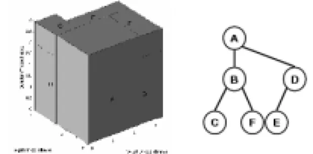
Figure 3: A compacted placement and the corresponding T-tree.

2.1.2. From a Compacted Placement to its T-tree

Given a compacted placement, we can represent it by a unique T-tree. A placement is said to be compacted if and only if no module can be moved along its X-, Y- or T- directions while other modules

are fixed. The root of the tree corresponds to the task on the origin (bottom-left) of a placement. We construct a T-tree for a compacted placement in a DFS manner: Starting from the root, we recursively construct the left sub-tree, then the middle sub-tree, and finally the right sub-tree. Let Li denote the set of

tasks that are adjacent to yi in the T+ direction. The

left child of node ni corresponds to the lowest task of

Li in the X-Y plane. The middle child of node ni

corresponding to the first task in the Y+ direction, with

its t-coordinate equal to that of ni's. The right child

of node ni represents the first task in the X+ direction,

with its y- and t-coordinate equal to those of ni's. A

compacted placement can be transformed to its corresponding T-tree in linear time. Figure 3 shows a compacted placement and its corresponding T-tree.

2.1.3. From a T-tree to its Placement

Now we describe the packing method for a T-tree. The t-coordinate of each module can be easily obtained by traversing the T-tree in the DFS order. If node nj is the left child of node ni, tj = ti + Ti;

otherwise, tj = ti. Once the t-coordinates are fixed,

we can utilize the existing tree solutions in [5] and [3] to compute y coordinates. We first decompose a T-tree into a set of binary trees. The T-tree decomposition process is shown in Figure 4. Starting from the root, we traverse a T-tree in the DFS order. When we encounter a node which has the right child, nb in the

example shown in Figure 4, we decompose the tree into two trees: one is the right sub-tree of nb, and the

other is the original tree without the right sub-tree of nb. The same decomposition procedure is applied to

each sub-tree until a leaf node is encountered. For each binary tree, we adopt the contour data structure presented in [5] and [3] to determine the y-coordinate of each module. The contour structure is a double-linked list of modules that records the contour line in current compaction. To compute x coordinates, we maintain a list lst to store all tasks whose t- and y-coordinates are already determined. The x-coordinate of task vi is equal to maxx'k {the

projections of vk and vi are overlapped on the Y-T

plane | k is in lst }.

Figure 4: The T-tree decomposition process.

2.2. Temporal Floorplanning Algorithm

Our floorplanning algorithm is based on the simulated annealing method [8]. The cost function Φ used in the algorithm is given by

Φ = αV + βW + γO,

where V stands for the volume of the placement, W is the total wirelength, O is the reconfiguration and communication overheads, and α , β , δ are user-specified constants. Given a T-tree (a feasible solution), we perturb the T-tree to obtain another feasible T-tree by using the following three operations:

Move: move a task to another place. Swap: swap two tasks.

Rotate: rotate a task.

2.2.1. Feasibility Detection and Tree

Re-construction

To maintain the temporal orderings among tasks, we need to guarantee that a T-tree meets all the precedence constraints after each perturbation. For

the three operations mentioned above, Move and Swap might violate the temporal constraints. Therefore, in this section, we describe how to examine the feasibility of a T-tree and the procedure to re-construct a T-tree to meet the precedence constraints.

Based on the structure of the T-tree, we know that if node nj is in the left sub-tree of ni's, task vj must be

executed after task vi. Therefore, to ensure all the

precedence constraints are not violated, a node nk must

be placed in the left sub-tree of np, where np has the

latest ending time among the tasks that must be executed before task vk.

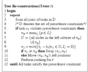
Once we identify a node that violates the precedence constraint, we re-construct the T-tree to remove the violation conditions. Assume task vi

violates precedence constraints and vp is the task that

has the latest ending time in Ii. Let U = {all nodes in the left sub-tree of np}∪{np}. In U, we look for a

node nj that minimizes |tj - ti| with Ij = empty set. If nj

≠np, ni is swapped with nj; otherwise, it means that nj

= np or Ij ≠empty set. In this case, we move ni to

the np's left position. The tree re-construction

process is summarized in Figure 5.

Figure 5: Summary of tree re-construction process.

3. Fixed-area Floorplanning:

For fixed-outline floorplanning, the area of the reconfigurable device is fixed. Let Wf/Hf and Wp/Hp

denote the width and height of a reconfigurable device and a placement, respectively. A feasible placement of fixed-outline floorplanning must satisfy the outline constraint; that is Wp ≤ Wf and Hp ≤ Hf. Therefore,

we consider excessive volumes of a placement in the objective function for the fixed-outline floorplanning problem. The new objective functionΦ’is:

Φ’=αV + βW + γO+ δF,

where δ is also a user-specified constant, and F is given in the following equation:

F = min((max(Wp-Wf, 0) × Hp × Time) + (max(Hp

-Hf, 0) ×Wp ×Time), (max(Wp-Wf, 0) × p × Time)

+ \max(Hp - Hf, 0) × Wp × Time)),

where Time is the total execution time for a placement. Since the whole design can be rotated by 90 degrees, we choose the smaller excessive volume of

two orthogonal placements.

Besides considering the excessive volume in the objective function, we bias the selection of the destination of the Move operations based on the value

n

k

, where k is the number of infeasible placements in the last n iterations. In this report, we set n equal to 500. A large

n

k

value indicates that the placement is not easy to fit into the device area; therefore, we should try to place a module along the$t direction to increase the success probability. In contrast, if the

n

k

value is small, we should try to place a module in the x or y direction to minimize the task execution time.

五､

成果 (Publications)

1. P.-H. Yu, C.-L.Yang, Y.-W. Chang, and H.-L. Chen, "Temporal floorplanning using 3D-subTCG," Proc. ASP-DAC, pp. 725--730, Yokohama, Japan, January 2004. (Nominated for Best Paper)

2. P.-H. Yu, C.-L. Yang, and Y.-W. Chang, ``Temporal floorplanning using 3D transitive closure sub-graphs," in revision, IEEE Trans. VLSI Systems, 2004.

3. P.-H. Yuh, C.-L. Yang, and Y.-W. Chang, ``Temporal Floorplanning using the T-tree Formulation," submitted to ICCAD 2004.

六

､

參考文獻

[1] Atmel, ``AT40K05102040AL_Complete,'' Atmel, Inc. [2] K. Bazargan, R. Kastner, and M. Sarrafzadeh, ``Fast Template

Placement for Reconfigurable Computing Systems,'' IEEE Design & Test of Computers, vol. 17, no. 1, pp. 68--83, Mar. 2000.

[3] Y.-C. Chang, Y.-W. Chang, G.-M. Wu, and S.-W. Wu, ``B*-trees: A new representation for non-slicing floorplan,'' Proc. DAC, pp. 458-462, June 2000.

[4] S. P. Fekete, E. Kohler, and J. Teich, ``Optimal FPGA Module Placement with Temporal Precedence Constraints,'' Proc. DATE, pp. 658-665, Mar. 2001.

[5] P.-N. Guo, C.-K. Cheng, and T. Yoshimura, ``An O-tree representation of non-slicing floorplan and its application,'' Proc. DAC, pp. 268-273, June 1999.

[6] S. Hauck,``The Roles of FPGAs in Reprogrammable Systems,'' Proc. the IEEE, vol.86, no. 4, pp. 615--639, Apr. 1998. [7] S. Hauck, Z. Li, and E.J. Schwabe, ``Configuration

Compression for the Xilinx XC6200 FPGA,'' Proc of FCCM, pp. 138--146, 1998.

[8] S. Kirkpatrick, C. D. Gelatt, and M. P. Vecchi, ``Optimization by Simulated Annealing,'' Science, vol. 220, no. 4598, pp.671--680, May 1983.

[9] R. Tesser and W. Burleson, ``Reconfigurable Computing for Digital Signal Processing: A Survey,'' Journal of VLSI Signal Processing, Vol. 28, no. 1, pp. 7--27, May/June 2001. [10] Xilinx, ``XAPP151 Virtex Series Configuration

Architecture User Guide v1.5,'' Xilinx, Inc., Sep. 2000. [11] Xilinx ``Virtex-II Pro Platform FPGA User Guide,'' Xilinx,

Inc.

[12] P.-H. Yuh, C.-L. Yang, Y.-W. Chang, and H.-L. Chang, ``Temporal Floorplanning using 3D-subTCG,'' Proc. ASP-DAC, pp. 725--730, Jan. 2004.