An Effective Mining Approach for Up-to-date Patterns

An Effective Mining Approach for Up-to-date

Patterns*

Tzung-Pei Hong1,2, Yi-Ying Wu3 and Shyue-Liang Wang4

1

Department of Computer Science and Information Engineering

3

Department of Electrical Engineering

4

Department of Information Management

National University of Kaohsiung, Kaohsiung, 811, Taiwan

2_{Department of Computer Science and Engineering}

National Sun Yat-sen University, Kaohsiung, 804, Taiwan

Abstract

Mining association rules is most commonly seen among the techniques for knowledge discovery from databases (KDD). It is used to discover relationships among items or itemsets. Furthermore, temporal data mining is concerned with the analysis of temporal data and the discovery of temporal patterns and regularities. In this paper, a new concept of up-to-date patterns is proposed, which is a hybrid of the association rules and temporal mining. An itemset may not be frequent (large) for an entire database but may be large up-to-date since the items seldom occurring early may often occur lately. An up-to-date pattern is thus composed of an itemset and its up-to-date lifetime, in which the user-defined minimum support threshold must be satisfied. The proposed approach can mine more useful large itemsets than the conventional ones which discover large itemsets valid only for the entire database. Experimental results show that the proposed algorithm is more effective than the traditional ones in discovering such up-to-date temporal patterns especially when the minimum support threshold is high.

Keyword: data mining, temporal patterns, up-to-date patterns, lifetime.

from log data”, presented at the IEEE International Conference on Granular Computing, 2008, China,

1.

Introduction

Knowledge discovery in databases (KDD) is to identify effective, coherent, and

useful information in large databases [10]. Through years of research in KDD, a

variety of data-mining techniques have been developed. According to the type of

databases processed, the mining approaches may be classified as working on

transaction databases, temporal databases, relational databases, multimedia databases,

and stream database, among others. There are also many mining methods proposed in

KDD, such as techniques for association rules, classification rules, clusters, sequential

patterns and so on. In particular, association rules have been most used in KDD

[3][4][8][11][12][14][15]. They are used to describe correlation relationships among

items or itemsets in transactional databases and have successful applications in many

areas.

Many algorithms based on the Apriori algorithm [1], which generated candidate

itemsets in a top-down level-wise process, were proposed to mine association rules.

When the percentage of transactions containing a candidate itemset is greater than or

equal to a user-specified minimum support threshold, the itemset is called as a

frequent (large) one and thought of as possessing correlation relationships among the

items included.

recently. It is concerned with the analysis of temporal data and the discovery of

temporal patterns and the regularities in temporal datasets. It typically reveals ordered

correlation of itemsets in transactions along with time. For example, consider a

database from a retail store. The sales of ice cream in summer and the sales of mitten

in winter should be higher than those in the other seasons. Such seasonal behavior of

specific items can only be discovered when a proper window size is chosen for the

mining process [6]. But a fixed window size may also hide some information about

the items.

In this paper, the concept for up-to-date patterns is described. Each itemset is

attached an up-to-date lifetime, in which the user-defined minimum support threshold

must be satisfied. In some cases, an itemset may not be frequent (large) for an entire

database but may be large up-to-date since the items seldom occurring early may

often occur lately. The up-to-date patterns thus include the itemsets which are

frequent for a flexible period of time from the current to the oldest past time.

Up-to-date patterns are practical in the field of data mining because they can provide

more useful information for the current usage than traditional ones. For example, the

counts of be mined patterns by up-to-date approach are larger than traditional data

mining, consequently, we can find more effective association rules. Also, Up-to-date

announced product such as i-phone may not be discovered as a frequent item from the

whole market transaction database. It may, however, be mined in time by the

proposed approach. Market managers can thus make effective decisions for marketing

strategy.

The remainder of this paper is organized as follows. Related works are reviewed

in Section 2. The up-to-date patterns from a log database and the proposed mining

algorithm are described in Section 3. An example to illustrate the proposed algorithm

is given in Section 4. Experiments for verifying the effectiveness of the above

approach are stated in Section 5. Conclusion and future work are given in Section 6.

2.

Review of Related Works

In this section, some related researches about mining association rules are briefly

reviewed. They are data mining for association rules and temporal data mining.

2. 1

Data Mining for Association Rules

Data mining technology has become increasingly important in the field of large

previously unknown and potentially useful knowledge, thus being able to help

managers make good decisions. Among the various types of databases and mined

knowledge, mining association rules from transaction databases is the most interesting

and popular [1][2][4][8][11][14][15][23]. In general, the process of mining

association rules can roughly be decomposed into two tasks:

(1) Finding frequent (large) itemsets satisfying a user-specified minimum support

threshold from a given database, and

(2) Generating interesting association rules satisfying a user-specified minimum

confidence threshold from the frequent itemsets found.

A variety of mining approaches based on the Apriori [3] algorithm were proposed,

such as DIC [13], DHP [12], Sampling, and FP-Growth [9]. Each of them was

designed for a specific problem domain, a specific data type, or for improving its

efficiency.

2. 2

Temporal Data Mining

Association-rule mining discovers unordered correlations between items from a

given database. However, temporal data mining reveals ordered correlations from

analysis of temporal data to find out temporal patterns and regularity from a set of

data with time. Temporal patterns can be discovered in a variety of forms, like

sequential association rules [5], periodical association rules [23], cyclic association

rules [19], and calendar association rules [18].

The calendar time expression [22] is widely used to specify the features of

temporal patterns. A calendar time expression is composed of calendar units in a

specific calendar and may represent different time features, such as an absolute time

interval over the time domain, a periodic time over the time domain, or a periodic

time within a specific time period. However, it is very difficult to choose a right

period of time such that the associations of particular interest can be found from the

transaction data. Besides, since different items may have different exhibition periods

in a log database, considering a fixed window size of each item might not lead to a

fair measurement. Therefore in this paper, we propose a flexible algorithm with

different effective lifetimes for items, focusing on the most recent itemsets.

3.

The Proposed Approach for Mining Up-to-date Patterns from

Log Databases

information is usually important to making decisions. In traditional data mining, an

itemset may not be frequent (large) for an entire database but be large up-to-date since

the items occurring early may not occur lately. Finding up-to-date knowledge is thus

very interesting and practical in the field of data mining. The concept of up-to-date

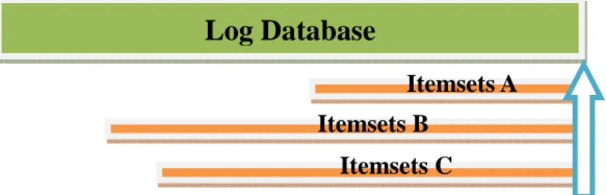
knowledge is shown in Figure 1.

For example, supposed user set a minimum support is 5%, and the database are

consist of 100 transactions, thus, an item can be extracted if the occurrence of the item

have to be larger than 5, in other words, if an item a occur only 4 times in the

database, it would not be extracted. On the contrary, we may extract the pattern like

({a}, <2008/4/21 10:00, 2008/4/22 13:30>) in this algorithm.

Figure 1: The concept of up-to-date knowledge

In Figure 1, an up-to-date pattern is a frequent (or called large) pattern with a

valid lifetime, in which the end point is the current time. Its start time will make the

lifetime as long as possible. It is a little like the concept of slide windows that it only

Log Database

Itemsets C Itemsets A Itemsets B

care the most recent itemsets in a fixed length. In this algorithm, we not only care

about the whole database, but also care the most recent itemsets in a non-fixed length.

Formally, an up-to-date pattern is defined as follows.

Definition: An up-to-date pattern is a pair ({Itemset}, <Lifetime>), where the

first term Itemset is a set of items and is large from a database duration the lifetime

which is the second term in the pair. The end value of the lifetime is the current time

and no other lifetime for the itemset may last longer than it.

According to the above definition, an algorithm is proposed in this section to find

all the up-to-date patterns from a given log database. It first translates the log database

into an item-oriented bit-map representation to speed up the execution in the later

mining process and then extracts large itemsets valid with the longest lifetime from

the past to the current time. The proposed approach can mine more useful large

itemsets than the conventional ones which discover large itemsets valid only for the

entire database. Before the algorithm is described, the notation used in this paper is

first defined below.

D: the log database;

n: the number of transactions in D; I: an item or an itemset;

T(I): the number of occurrences of itemset I in D; Min_Sup: the support threshold for large itemsets;

r: a parameter that used to keep the current number of items in the itemset;

Si: the short-lifetime i-itemsets in which an itemset needs to shorten its lifetime to be

large;

Li: the set of large i-itemsets from D;

Ci: the set of all candidate i-itemsets from D;

Timelist(I): the set of transaction IDs in which itemset I appears; First(I): the first transaction ID in Timelist(I);

Lifetime(I): the period of time in which I is large.

3. 2

The Proposed Algorithm

The details of the proposed algorithm are described below.

Mining up-to-date patterns from a log database:

INPUT: A log database D with n transactions stored in the order of transaction time,

each of which includes transaction ID, transaction time, items, and among

others, and a minimum-support threshold Min_Sup.

OUTPUT: A set of up-to-date itemsets with their corresponding lifetimes.

STEP 1: Transform the given log database into the item-oriented bitmap

transaction contains I and is set as 0 otherwise.

STEP 2: For each item I, find out from the bitmap representation the transactions in

which item I appears. Let Timelist(I) represents the above set of

transactions for I in the order of transaction IDs. Calculate the count of each

item I in Timelist(I) as the number of 1’s and put the count into T(I).

STEP 3: Check whether the count T(I) of each item I is larger than or equal to the

minimum count, which is n*Min_Sup. If it is, put({I}, <1, n>) in the large

1-patterns (L1); If it is not, put the item I in the set of short-lifetime

1-itemsets (S1).

STEP 4: For each item I in the set of S1, do the following substeps.

Substep 4-1: Set First(I) as the first transaction ID in Timelist(I).

Substep 4-2: Calculate whether the item I is frequent during the lifetime

<First(I), n> by thefollowingformula:

( )

( )

If the item I satisfies the above condition, then put the pattern

({I}, <n – (T(I)/Min_Sup) + 1, n>) in L1; Otherwise, set

First(I) as the next transaction ID in Timelist(I), decrease the

count of T(I) by one, and repeat this substep until T(I) is equal

STEP 5: Set r = 1, where r is used to keep the current number of items in the itemset

to be processed.

STEP 6: Generate the candidate set Cr+1 from Lr in a way similar to the Apriori

algorithm, except that the start ID in the possible lifetime of an

(r+1)-itemset in Cr+1 is the maximum of the start IDs of the r-itemsets

forming the (r+1)-itemset.

STEP 7: For each (r+1)-itemset I in Cr+1, use the AND operator on the possible

lifetime bits and mask the other bits to find Timelist(I) from the bitmap

representation.

STEP 8: Find the large (r+1)-pattern (Lr+1) of Iin a way similar to STEPs 3 and 4.

STEP 9: If Lr+1 is null, do the next step; Otherwise, set r = r + 1 and repeat STEPs 6

to 8.

STEP 10: In order to reduce the number of large pattern and save the memory space,

keep the closed frequent itemsets to substitute for all large pattern. Thus,

no superset that is frequent with the same lifetime. Transform the

transaction IDs in the lifetimes into the actual occurring times and output

the transformed up-to-date patterns to users.

or hashes, can be used to speed-up the execution. Besides, after the patterns are found,

the association rules can also be easily derived.

4.

An Example

In this section, an example is given to illustrate the proposed up-to-date mining

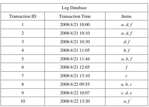
algorithm from a log database. Table 1 shows the log database to be used in the

example. The database contains 10 transactions and 6 items, denoted a to f.

Table 1: Thelog databasein the example

Log Database

Transaction ID Transaction Time Items

1 2008/4/21 10:00 a, d, f 2 2008/4/21 10:10 a, d, f 3 2008/4/21 10:30 d, f 4 2008/4/21 11:05 b, f 5 2008/4/21 11:46 a, b, f 6 2008/4/21 12:05 f 7 2008/4/21 13:10 c 8 2008/4/22 09:55 a, b, c 9 2008/4/22 10:07 c, d, e 10 2008/4/22 13:30 a, f

Assume the minimum-support threshold is set at 50%. The proposed algorithm

STEP 1: The given log database is first transformed into the item-oriented bitmap

representation. Take item a as an example. It appears in transactions 1, 2, 5,

8 and 10, and the corresponding bits are thus set as 1. After STEP 1, the

obtained bitmap representation for the transactions in Table 1 is shown in

Table 2.

Table 2: The item-oriented bitmap representation in the example

1 2 3 4 5 6 7 8 9 10 a 1 1 0 0 1 0 0 1 0 1 b 0 0 0 1 1 0 0 1 0 0 c 0 0 0 0 0 0 1 1 1 0 d 1 1 1 0 0 0 0 0 1 0 e 0 0 0 0 0 0 0 0 1 0 f 1 1 1 1 1 1 0 0 0 1

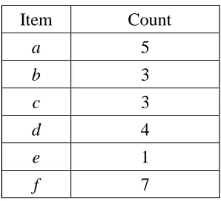
STEP 2: The transactions in which item I appears can be easily found out from the

bitmap representation. Take item a as an example. It can be easily obtained

Timelist(a) is thus {1, 2, 5, 8, 10}. Besides, the count T(I) of each item I can

be easily found from the number of 1’s in its bit map. The results after Step

2 are shown in Table 3.

Table 3: The counts of the items in the example

Item Count a 5 b 3 c 3 d 4 e 1 f 7

STEP 3: The count T(I) of each item I is compared with the minimum count. In the

example, since the minimum support is set at 50% and there are ten

transactions, the minimum count is thus 10*0.5, which is 5. Among the

items, the counts of items a and f are larger than the minimum count. They

are thus frequent for the whole database and the two patterns, ({a}, <1, 10>)

and ({f}, <1, 10>) are put in L1. On the contrary, the counts of items b, c, d

and e are smaller than the minimum count, they are then put into the set of

short-lifetime 1-itemsets (S1). Thus S1 = {b, c, d, e}.

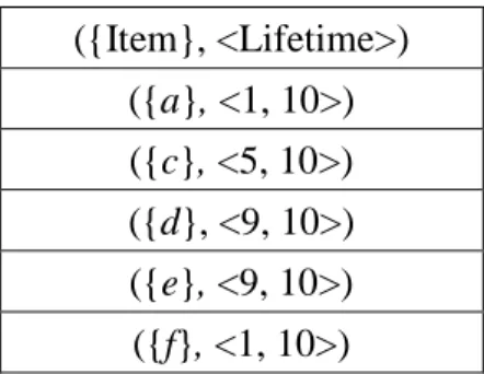
STEP 4: The following two substeps are done for each item I in the set of S1.

Timelist(I). Take item c as an example to illustrate the step. It

can be easily found from Table 2 that First(c) is 7.

Substep 4-2: The item I is checked during the lifetime <First(I), n> by the

given formula:

( )

( )

In the example for item c, the range of the transactions with

item c is 10-7+1 (= 4), which is less than the count T(c) of item

c divided by the minimum support (3/0.5). Item c is then a large

1-pattern. Its start ID is calculated as 10- 3/0.5+1, which is 5,

according to the formula in the algorithm. The pattern ({c}, <5,

10>) is thus put in L1. For item b, the range of the transactions

with item b is 10-4+1 (= 7), which is larger than the count T(b)

of item b divided by the minimum support (3/0.5). The variable

First(b) is then moved to the next transaction ID in Timelist(b),

which is 5. The count of b is decreased by one, becoming 2,

and Substep 4-2 is repeated again. In this example, item b is

found not an up-to-date pattern until T(b) is equal to zero. After

Table 4: The obtained up-to-date 1-patterns in the example ({Item}, <Lifetime>) ({a}, <1, 10>) ({c}, <5, 10>) ({d}, <9, 10>) ({e}, <9, 10>) ({f}, <1, 10>)

STEP 5: The variable r isset at 1, where r is used to keep the current number of items

in the itemset to be processed.

STEP 6: The candidate set C2 is generated from L1. The start ID of a 2-itemset is the

maximum of the start IDs of the two items in the 2-itemset. Take the

candidate 2-itemset {ac} as an example. Lifetime(ac) is generated from

Lifetime(a) (<1, 10>) and Lifetime(c) (<5, 10>). Since the maximum of the

two start IDs is 5, Lifetime(ac) is thus<5, 10>. After STEP 6, the resulting

candidate set C2 is shown in Table 5.

Table 5: The resulting candidate set C2 in the example

({Itemset}, <Lifetime>) ({ac}, <5, 10>) ({ad}, <9, 10>) ({ae}, <9, 10>) ({af}, <1, 10>) ({cd}, <9, 10>) ({ce}, <9, 10>) ({cf}, <9, 10>)

({de}, <9, 10>) ({df}, <9, 10>) ({ef}, <9, 10>)

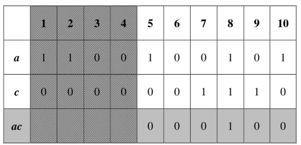
STEP 7: For each 2-itemset I in C2, its Timelist(I) is found from the bitmap

representation by the AND operation. Take the candidate 2-itemset {ac} as

an example. Since Lifetime(ac) is <5, 10>, only the ones from the 5-th to the

10-th bits for items a and c are operated, and the other bits are masked as 0.

The process is shown in Table 6.

Table 6: Finding Timelist(ac) in the example by the AND operation

1 2 3 4 5 6 7 8 9 10

a 1 1 0 0 1 0 0 1 0 1

c 0 0 0 0 0 0 1 1 1 0

ac 0 0 0 1 0 0

In the example, only the 8-th bit is 1 and thus only the 8-th transaction

needs to be further considered for the itemset {ac}. Take another candidate

2-itemset {af} as an example. Its possible lifetime is <1, 10>. The process is

Table 7: Finding Timelist(af) in the example by the AND operation

1 2 3 4 5 6 7 8 9 10

a 1 1 0 0 1 0 0 1 0 1

f 1 1 1 1 1 1 0 0 0 1

af 1 1 0 0 1 0 0 0 0 1

STEP 8: The itemset I is checked for whether it is large (in L2) in a way similar to

STEPs 3 and 4. Take the 2-itemset {ac} as an example. Its range of

transactions is 10-8+1 (= 3), which is larger than the count T(ac) of itemset

{ac} divided by the minimum support (1/0.5). The count of {ac} is then

decreased by one, becoming 0. The loop then stops for the itemset {ac} and

it is not a large pattern. For the 2-itemset {af}, its range of transactions is

10-1+1 (= 10), which is larger than the count T(af) divided by the minimum

support (4/0.5). The variable First(af) is then moved to the next transaction

ID in Timelist(af), which is 2. The count of {af} is decreased by one,

becoming 3. Substep 4-2 is then repeated again. Finally, the large 2-pattern

({af}, <9, 10>) is found and put in L2. After the step, the results are shown

Table 8: The obtained up-to-date 2-patterns in the example ({Itemset}, <Lifetime>) ({af}, <9, 10>) ({cd}, <9, 10>) ({ce}, <9, 10>) ({de}, <9, 10>)

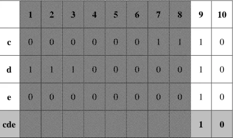
STEP 9: Since L2 is not null, r is set at 2 and STEPs 6 to 8 are repeated. In the

example, the only candidate 3-itemset is ({cde}, <9, 10>). Its Timelist is

then found from the bitmap representation by the AND operation. The

process is shown in Table 9.

Table 9: Finding Timelist(cde) in the example by the AND operation

1 2 3 4 5 6 7 8 9 10

c 0 0 0 0 0 0 1 1 1 0

d 1 1 1 0 0 0 0 0 1 0

e 0 0 0 0 0 0 0 0 1 0

cde 1 0

The itemset {cde} is then checked for whether it is large (in L3) in a way

similar to STEPs 3 and 4. The 3-pattern ({cde

}

The next step is then executed.

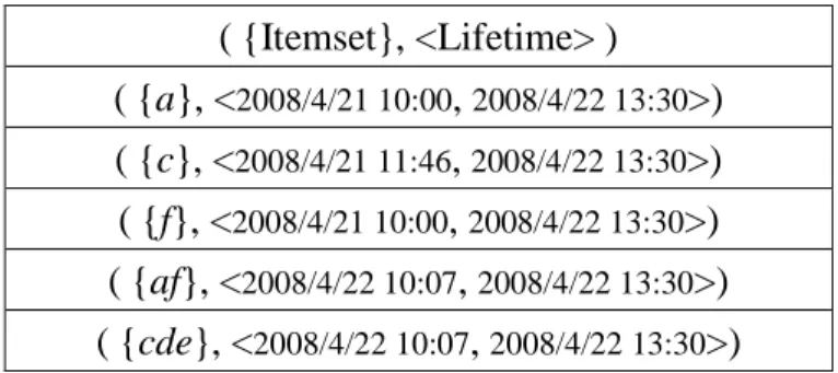
STEP 10: All the up-to-date patterns are found. And check whether up-to-date

patterns are closed frequent itemsets. In the example, up-to-date 3-patterns

({cde

}

2-patterns ({cd}, <9, 10>), ({ce}, <9, 10>), ({de}, <9, 10>) and up-to-date

1-patterns ({d}, <9, 10>), ({e}, <9, 10>), that with the same lifetime. On

the contrary, the up-to-date 1-patterns ({c}, <5, 10>) is keep, because there

are no superset that is frequent with the same lifetime. All the transaction

IDs in the lifetime are transformed into the actual occurring times

according to the database, and the patterns are then output to users. The

final up-to-date patterns are shown in Table 10

Table 10 The final up-to-date patterns in the example

( {Itemset}, <Lifetime> ) ( {a}, <2008/4/21 10:00, 2008/4/22 13:30>) ( {c}, <2008/4/21 11:46, 2008/4/22 13:30>) ( {f}, <2008/4/21 10:00, 2008/4/22 13:30>) ( {af}, <2008/4/22 10:07, 2008/4/22 13:30>) ( {cde}, <2008/4/22 10:07, 2008/4/22 13:30>)

From the results, it can be seen that each itemset may have its own valid lifetime

the original mining algorithms. Since up-to-date knowledge is usually important for

making decisions, the proposed approach is expected to provide some effective

reference values to users or managers.

5.

Experimental Results

In the section, we describe the implementation details of the proposed algorithm

for mining up-to-date patterns from a log database. They were implemented in C on

an AMD Athlon 64 Processor 3200+ personal computer with 1.99GHz and 1GB

RAM. The IBM database, T10I4D100K, was used to verifythe proposed approach. In

the database, the size of a transaction was 10, the size of potential maximal large

itemsets was 4, and the number of transactions was 100000.

In order to make an efficient execution, the bitmap data structure was used to

speed up both the I/O access and the program execution. The proposed approach was

compared to the traditional method that mined frequent itemsets without up-to-date

patterns. Different minimum support values were set in the experiments.

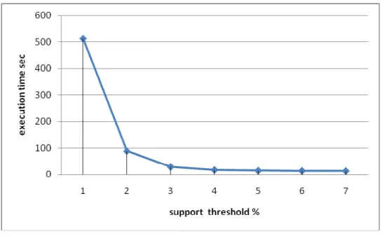
In the first experiment, the relationships between execution times and minimum

supports are shown. The minimum supports varied from 1% to 7%. The results are

Figure 2:The relationships between execution times and support threshold

It can be observed that the curve of execution times is close to zero when the support

threshold is above 3% for the dataset. The execution times increase sharply when the

support threshold changed from 2% to 1%. This is because when the support

threshold is low, the number of up-to-date patterns dramatically increased.

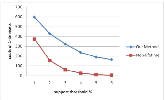
Next, the relationships between the numbers of 1-itemsets for different minimum

support thresholds are shown in Figure 3. It is clear that the number of frequent

itemsets discovered by the proposed mining algorithm for up-to-date patterns was

Figure 3: The relationships between numbers of 1-itemsets and support thresholds

The relationships between the numbers of 2-itemsets and 3-itmesets for different

minimum support thresholds are shown in Figures 4 and 5, respectively. It can be

observed that the counts of the 2-itemsets and 3-itemsets without up-to-date patterns

method are close to zero when the support threshold was set at above from 1%.

Restated, rare frequent 2-itemsets and 3-itemsets were generated. The same as before,

by the proposed method for up-to-date patterns, the number of frequent itemsets

discovered are much more than that by the traditional one. Besides, the rules from a

high support threshold are usually more important than those form a low support

threshold. When the support threshold increased, more up-to-date patterns with

shorter lifetimes would be generated. Since finding patterns with a large support

can find more useful knowledge than the traditional one for a large support threshold.

Figure 4: The relationships between numbers of 2-itemsets and support

thresholds

Figure 5: The relationships between numbers of 3-itemsets and support

6.

Conclusion and Future Work

In this work, we have described the concept of up-to-date temporal patterns and

have proposed an approach to discover such patterns from a temporal dataset. An

example illustrating the proposed algorithm is also given. Experimental results show

that the proposed algorithm is more effective than the traditional mining methods in

discovering such up-to-date temporal patterns. Especially when the large support is

high, the proposed approach has much more association rules than the traditional ones,

which derive very rare rules. In the future, we may study using appropriate data

structures to speed up the execution time. We will also further investigate the

enhancement of the proposed up-to-date model.

References

1. R. Agrawal, T. Imielinksi and A. Swami, “Mining association rules between sets

of items in large database,“ The ACM SIGMOD Conference, Washington DC,

USA, 1993.

2. R. Agrawal, T. Imielinksi and A. Swami, “Database mining: a performance

perspective,” IEEE Transactions on Knowledge and Data Engineering, Vol. 5, No.

3. R. Agrawal and R. Srikant, “Fast algorithm for mining association rules,” The

International Conference on Very Large Data Bases, pp. 487-499, 1994.

4. R. Agrawal, R. Srikant and Q. Vu, “Mining association rules with item

constraints,” The Third International Conference on Knowledge Discovery in

Databases and Data Mining, Newport Beach, California, 1997.

5. R. Agrawal, R. Srikant, “Mining sequential patterns,” The 7th International

Conference on Data Engineering, pp. 3-14, 1995.

6. J. F. Roddick and M. Spiliopoulou, “A survey of temporal knowledge discovery

paradigms and methods,” IEEE Transactions on Knowledge and Data

Engineering, pp. 750-767, 2002.

7. H. Mannila, M. Informatic, I. Stadtwaldt and H. Toivonen, “On an algorithm for

finding all interesting sentences,” The 13thEuropean Meeting on Cybernetics and

Systems Research, pp. 973-978, 1996.

8. J. Han and Y. Fu, “Discovery of multiple-level association rules from large

database,” The 21st International Conference on Very Large Data Bases, Zurich,

Switzerland, pp. 420-431, 1995.

9. J. Han, J. Pei, and Y. Yin, “Mining frequent patterns without candidate

generation,” ACM SIGMOD Conference, pp. 1-12, 2000.

10. W. J. Frawley, G. P. Shapiro and C. J. Matheus, “Knowledge discovery in

databases: an overview,” The AAAI Workshop on Knowledge Discovery in

Databases, pp.1-27, 1991.

11. H. Mannila, H. Toivonen and A. Inkeri Verkamo, “Efficient algorithm for

discovering association rules,” The AAAI Workshop Knowledge Discovery in

Databases, pp. 181-192, 1994.

12. J. S. Park; M. S. Chen; P. S. Yu, “Using a hash-based method with transaction

Data Engineering, pp.812-825, 1997.

13. S. Brin, R. Motwani, J. D. Ullman and S. Tsur, “Dynamic itemset counting and

implication rules for market basket data,” The ACM SIGMOD Conference, Tucson,

Arizona, USA, pp. 255-264, 1997.

14. R. Srikant and R. Agrawal, “Mining generalized association rules,” The 21st

International Conference on Very Large Data Bases, Zurich, Swizerland, pp.

407-419, 1995.

15. A. Savasere, E. Omiecinski and S. Navathe, “An efficient algorithm for mining

association rules in large databases,” The ACM VLDB Conference, pp. 432-444,

1995.

16. B. Liu, W. Hsu and Y. Ma, “Mining association rules with multiple minimum

supports,” The 1999 International Conference on Knowledge Discovery and Data

Mining, pp.337-341, 1999.

17. K. Wang, Y. H and J. Han, “Mining frequent itemsets using support constraints,”

The 26th International Conference on Very Large Data Bases, pp. 43-52, 2000.

18. Y. Li, P. Ning, X. S. Wang and S. Jajodia. “Discovering calendar-based temporal

association rules,” Data & Knowledge Engineering, pp. 193-218, 2003.

19. B. Ozden, S. Ramaswamy and A. Silberschatz. “Cyclic association rules,” The

14th International Conference on Data Engineering, Orlando, Florida, USA, pp.

12-421, 1998.

20. J. W. Lee, Y. J. Lee, H. K. Kim, B. H. Hwang and K. H. Ryu. “Discovering

temporal relation rules mining from interval data,” The First EurAsian Conference

on Information and Communication Technology (Eurasia-ICT 2002), Shiraz, Iran,

pp, 57-66, 2002.

21. J. M. Ale and G. H. Rossi. “An approach to discovering temporal association

294-300, 2000.

22. K. Verma, O.P. Vyas and R. Vyas. “Temporal approach to association rule mining

using T-tree and P-Tree,” Lecture Notes in Computer Science, Vol. 3587, 2005, pp.

651 – 659.

23. D. Li and J. S. Deogun, “Discovering partial periodic sequential association rules

with time lag in multiple sequences for prediction,” Lecture Notes in Computer

Sciences, Vol. 3488, 2005, pp. 332-341.

24. M. S. Chen, J. Han and P. S. Yu, “Data mining: An overview from a database

perspective,” IEEE Transactions on Knowledge and Data Engineering, Vol. 8, No.

6, 1996.

25. X. Chen, I. Petrounias and H. Heathfield, “Discovering temporal association rules

in temporal databases,” The International Workshop on Issues and Applications of