A novel cross-coupling control design for Bi-axis motion

A novel cross-coupling control design for Bi-axis motion

Yi-Ti Shih

_{, Chin-Sheng Chen}

_{, An-Chen Lee}

a_{Department of Mechanical Engineering, National Chiao Tung University, 1001 Ta Hsueh Road, Hsinchu, 300-10, Taiwan} b_{TECO Electric & Machinery Co. Ltd,Taiwan}

Received 23 April 2002; accepted 17 July 2002

Abstract

A new structure of cross-coupling controller for precise tracking in motion control is proposed in this paper. When compared with the conventional cross-coupling system, this new structure has the advantage that the compensators in CCC have a simpler design process than conventional ones and so does its stability analysis. The proposed compensator (or controller) is evaluated and compared experimentally with a traditional uncoupled controller on a microcomputer controlled dual-axis positioning system. The experimental results show that the new structure of cross-coupling controller remarkably reduces contour error. In addition, this new controller can be implemented easily on a majority of motion systems in use today via reprogramming the reference position command subroutine.

 2002 Elsevier Science Ltd. All rights reserved.

Keywords: Contour error; Cross-coupling controller

1. Introduction

Accurate trajectory control is a fundamental require-ment for modern manufacturing systems, which is especially true for CNC machine tools. One can improve any single axial positioning accuracy by applying vari-ous control strategies such as a large P gain controller, a feed-forward controller [1] and a ZPETC (zero phase error tracking controller) [2]. However, good tracking performance for each individual axis does not guarantee the reduction of the contour error for multi-axis motion [3]. The term ‘contour error’ representing, for example, the deviation of the cutter location from the desired con-tour path in a CNC machine, is defined as the error component orthogonal to the desired trajectory. Another method to reduce the contour error is the cross-coupling control. Koren [4] introduced a symmetrical structure of cross-coupling controller to improve the contour accu-racy. In his research, he considered the whole system as a single unit, instead of individual loops, and as a result, the influences of load disturbances and axis mismatch on system performance can be reduced.

∗ _{Corresponding author. Tel: +886-3-5728513; fax: +}

886-3-5725372.

E-mail address: [email protected] (A.-C. Lee).

0890-6955/02/$ - see front matter.2002 Elsevier Science Ltd. All rights reserved. PII: S 0 8 9 0 - 6 9 5 5 ( 0 2 ) 0 0 1 0 9 - 8

A typical cross-coupling controller essentially consists of an algorithm to calculate the contour error and a con-trol law to eliminate the contour error. Many concon-trol laws such as traditional PID control [3], optimal control [5], adaptive control [6], fuzzy logic control [7], and robust control (QFT design algorithm) [8] have been proposed to implement the CCC.

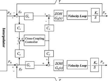
A typical conventional cross-coupling control system in the literature is shown in Fig. 1, where the CCC output is generated to modify feed drive (velocity command type). In this figure, Keis a scaling factor related to the

encoder resolution and gear ratio; T is the sampling time; Pdx and Pdy are the desired axial positions and

Pax and Pay are the actual positions for X and Y axes,

respectively; Gx and Gyare the position loop gains for

each axis. Exand Ey are the tracking errors; Cx and Cy

are variable gains related to the geometry of contour;

e is the contour error calculated by geometric

relation-ship. In the design of this type of CCC, the output of the CCC is decomposed and then injected into the loops in order to reduce the contour error.

The servo drives used in industry nowadays can be classified into three types of control mode: position mode, velocity mode, and torque mode. Each mode gives its merit and applicability and no one is dominant. This is why most suppliers provide these three control

Fig. 1. A typical structure of conventional CCC motion system.

modes for application engineers to choose. Although various control modes are available, the classical CCC, intending to modify the command of velocity-mode feed drive, is not able to cope with systems using the position-mode feed drive. In order to apply this advanced control scheme, we need a more generalized CCC structure and this becomes the motivation of this paper. Since the con-tour error is function of axial tracking errors, the authors believe that the modification of the position command is also a feasible way to reduce contour error. Specifi-cally, the output of the new CCC for each axis will directly feed back to modify reference position com-mand. As will be shown in later sections, the design of the proposed CCC will introduce a ‘contour error trans-fer function’, or CETF with the characteristics of a high pass filter. Its stop band should match to the bandwidth of the original single-axis position loop. Since the cas-cade compensation—the most commonly used controller configuration in industry—is adopted here for the single-axis position loop, the cut-off frequency of CETF is determined accordingly. The whole design procedure and stability analysis of the proposed CCC become very simple. Also, we will discuss the conditions of feasible cross-coupling controller and choose the pole-placement method to design a simple permissible PI-type CCC, which enables us to shape the dynamics of contour error. Additional constraints given by Jury’s criterion will limit the corner frequency of the CCC and allow us to find its stable region easily.

In the following, we will first derive different contour-error estimation equations for linear and circular con-tours according to the geometric relations between the desired and actual positions. The performance of cross-coupling controller will deteriorate when a path with a large curvature (such as a small circle) or at a high feed-rate occurs. Therefore, a more accufeed-rate contour error estimation equation for the circular motion is developed

here to cope with this situation. Then we will discuss how to determine of the stable region and to use the pole-placement method to design a PI-type compensator in consequence. Finally, the simulations and experiments are performed and discussed. They show a good consist-ency with each other and confirm the effectiveness of this CCC design.

2. Contour errors

In this section, two kinds of contouring motion are discussed here:

2.1. Linear contour [3]

The linear contour error can be determined by follow-ing equation:

e⫽ ⫺Exsinq⫹ Eycosq ⬅ ⫺ExCx⫹ EyCy (1)

where q is the angle between the line and the X-axis;

Exand Eyare the tracking errors of X and Y axes,

respect-ively.

2.2. Circular contour

The contour error for circular contour is the difference between the actual location to the center of the circle and the radius of the circle, and can be defined as

e⫽

冑

where q is the angle between the instantaneous tangent

at reference position and the X-axis. Eq. (2) can be further simplified by the Taylor series expansion as

e⫽ ⫺Ex

冉

冊

冉

冊

2R(Exsinq⫺Eycosq)

2 ⫹f(Ex,Ey)

R2 ⫹ …

Generally, it is true that axial tracking errors are much smaller than the radius of circle. Thus, the high-order terms of Ex, Eyin Eq. (3) can be neglected, resulting in

Eq. (1). The same expression of contour error estimation for both linear and circular contours is widely adopted before [9,10]. But in the case of small radius or high speed circular contouring, instead of Eq. (1), the follow-ing Eq. (4) should be used to calculate the contour error. Otherwise, the reduction of contour error cannot be achi-eved. This is confirmed by simulation and experiment at section 5. e⫽ ⫺Ex

冉

冊

冉

冊

2R(Exsinq⫺Eycosq)

2⫽ ⫺E

x

冉

⫺Excosq⫹ Eysinq

⫹Excosq⫹ Eysinq

2R sinq

冊

Cx⫽ sinq⫺

Excosq⫹ Eysinq

2R cosq. (5a)

Cy⫽cosq⫹ Excosq⫹ Eysinq

2R sinq (5b)

Eq. (4) is valid for both the linear and circular contours, since, for linear contour case, we can let R in the above equation be infinity.

3. Proposed CCC structure

In this section, the contour errors for both an uncoupled system and a cross-coupled one are developed. For ease of presentation, the notation of velo-city loop together with the position integrator is defined as Lv(z⫺1) in Fig. 2. The forward and feedback velocity

loop controllers, Cvfw(z⫺1) and Cvfb(z⫺1), are designed

to handle the velocity performance and disturbance rejection; Gi(s) represents

Ke

s shown in Fig. 1, and Gp(s) is the mathematical model of plant. Note that the

following derivations are based on Z-domain analysis, although all (z⫺1)s in the argument of functions are omit-ted for clarity in expression.

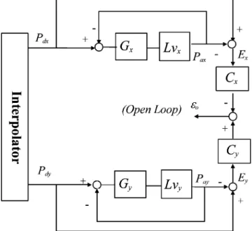
3.1. The uncoupled motion control system

A dual-axis uncoupled motion control system is presented in Fig. 3. The contour error defined for this uncoupled (open) system is

eo⫽ ⫺ExCx⫹ EyCy. (6)

From the figure, tracking errors ExandEyfor the two axes

can be easily obtained by following deductions:

Fig. 2. The function block notation for velocity loop and the inte-grator.

Fig. 3. An uncoupled motion control system.

Ex⫽ Pdx⫺Pax⫽ Pdx⫺ GxLvx 1⫹ GxLvxPdx (7a) ⫽ Pdx 1⫹ GxLvx Ey⫽ Pdy 1⫹ GyLvy. (7b)

Substituting Eq. (7) into Eq. (6), we obtain the contour error of the uncoupled system, or

eo⫽ ⫺ExCx⫹ EyCy⫽ ⫺ CxPdx

1⫹ GxLvx (8)

⫹ CyPdy

1⫹ GyLvy.

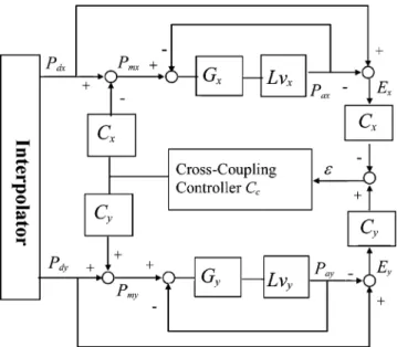
3.2. The proposed cross-coupled motion control system

By using the cross-coupling controller Cc to couple

the two axes, we propose the structure as shown in Fig. 4, where Pmx and Pmy are the modified position

com-mands of each axis. The cross-coupling control forms two extra position loops, which are used to modify the position command of each axis. Based on the concept of cascade control, it is clear that the design of original tracking system does not affect these two outer loops. The following equations can be easily obtained form Fig. 4,

e⫽ ⫺ExCx⫹ EyCy (9)

Ex⫽ Pdx⫺Pax⫽

Pdx⫹ eCcCxGxLvx

Fig. 4. The proposed structure of cross-coupled control system.

Similarly,

Ey⫽Pdy⫺eCcCyGyLvy

1⫹ GyLvy . (10b)

Substituting Eq. (10) into Eq. (9), we obtain

e⫽ ⫺ExCx⫹ EyCy⫽ ⫺ CxPdx⫹ eCcC 2 xGxLvx 1⫹ GxLvx (11) ⫹CyPdy⫺eCcC 2 yGyLvy 1⫹ GyLvy .

Rewrite Eq. (11) to obtain e as e⫽⫺(1 ⫹ GyLvy)Cx ⌬ Pdx⫹ (1⫹ GxLvx)Cy ⌬ Pdy (12) in which ⌬ ⫽ (1 ⫹ GxLvx)(1⫹ GyLvy)⫹ CcC2 xGxLvx(1 (13) ⫹ GyLvy)⫹ CcC 2 yGyLvy(1⫹ GxLvx).

Substituting Eq. (12) into Eq. (10), we get the following results, or Ex⫽ Pdx 1⫹ GxLvx⫺ CcC2xGxLvx(1⫹ GyLvy) (1⫹ GxLvx)⌬ Pdx (14a) ⫹CcCxCyGxLvx ⌬ Pdy Ey⫽ Pdy 1⫹ GyLvy⫺ CcC 2 yGyLvy(1⫹ GxLvx) (1⫹ GyLvy)⌬ Pdy (14b) ⫹CcCxCyGyLvy ⌬ Pdx.

Comparing Eq. (14) to Eq. (7), we find the last two terms in Eq. (14) are induced by cross-coupling control. If gain of Ccis small, the CCC will not influence the tracking

performance. How to design Ccto keep good contouring

performance will be discussed in the following section.

4. Design of the compensator of CCC

4.1. Design a PI compensator

Examining Eqs. (8) and (12), we can obtain the relationship between the contour errors of the coupled and un-coupled system, or

e⫽(1⫹ GxLvx)(1⫹ GyLvy)

⌬ eo. (15)

Furthermore, Eq. (15) can be rearranged as,

e⫽ 1 1⫹ CcP eo (16) where P⫽C 2 xGxLvx(1⫹ GyLvy)⫹ C2yGyLvy(1⫹ GxLvx) (1⫹ GxLvx)(1⫹ GyLvy) . (17) ⫽ C2xGxLvx 1⫹ GxLvx ⫹ C2yGyLvy 1⫹ GyLvy

The similar functional relationship 1 1⫹ CcP

between the coupled and uncoupled systems is defined as the contour error transfer function (CETF) in Yeh and Hsu’s research [8]. In order for us to design Cc, understanding

‘what is P?’ is the first thing to do. By the rule of the cascade control, once the velocity controllers in Fig. 4 is tuned appropriately (i.e., the bandwidth of velocity loop is at least three times larger than that of the position loop and the step response behaves no oscillation), the velocity control loop can be simplified as unit gain, and

Lvx⫽ Lvy⫽

T

1⫺z⫺1. (18)

To simplify our analysis, let Gx⫽ Gy⫽ G, i.e., the two

axes have almost matched dynamics. We further define

Gv⫽ C2

x ⫹ C2y (19)

For linear contour, from Eq. (1) we get

Gv⫽ C2

x ⫹ C2y⫽ sin2q⫹ cos2q⫽ 1. (20)

For circular contour, if tracking errors Ex and Eyare

much smaller than the radius of curvature R, from Eq. (1), we get

Gv⫽ C2

x ⫹ C2y⫽ 1. (21)

For small radius circular motion, from Eq. (5), we get

Gv⫽ C2 x ⫹ C2y⫽ 1 ⫹

冉

冊

Although the second terms in Eq. (5) play an important role in contour error estimation under certain circum-stances which will be shown in section 5, it is convenient in the controller design phase to approximate Gvin Eq.

(22) to one. Thus, Eq. (17) can be reduced to

P⫽ G T Gv

1⫹ GT⫺z⫺1. (23)

When a matched but uncoupled system tracks a line or circle, the contour error will approach a constant after transience. Even if the dynamics of the two axial pos-itioning systems are not so matched, the major part of contour error still behaves like a low frequency signal. In order to reduce the steady-state contour error or the low frequency components, the CETF, or 1

1⫹ CcP

, is required to have a very low gain at low frequency range, which amounts to requiring |CcP| be maximum at low

frequency range. The simplest way is to let the control-ler Cccontain an integrator, resulting in the general form

of Q(z

⫺1₎

1⫺z⫺1, where Q(z

⫺1_{) is used to shape the CETF}

further to meet the designer’s requirements. Since the P is a first order rational function, the added integrator will make CETF become a second order system. The per-formance of this kind of system can be specified easily by two parameters. In consequence, a PI controller is chosen as the CCC compensator for the contour error correction, i.e., Q(z⫺1)contains only one zero (In Appen-dix A, the requirement and conditions forCc(s), F(s) and

P(s) are discussed in detail). The generalized

character-istic equation in Eq. (16) can be expressed as follows,

1⫹ Cc

GTGv

1⫹ GT⫺z⫺1⫽ 0. (24)

Let Kcp,Kci be the proportional and integral controller

gains respectively, then this standard discrete time con-troller can be expressed as

Cc(z⫺1)⫽ Kcp⫹ Kci

1

1⫺z⫺1. (25) By substituting Eq. (25) into (24), characteristic equation is rewritten as D(z)⫽ z2⫺ 2⫹ GT ⫹ GTGvKcp 1⫹ GT ⫹ GTGv(Kcp⫹ Kci) z (26) ⫹ 1 1⫹ GT ⫹ GTGv(Kcp⫹ Kci) ⫽ 0.

For this second order system, we can design it by the pole-placement method. Letx, wnbe the two parameters

similar to damping ratio and natural frequency of a stan-dard second order system, then the parameters of this compensator are Kcp⫽ 2(ezw_nT_·cos(T·w n

冑

冑

The definition of BIBO stability as mentioned in books written by Yeh [11] or Goodwin etc. [12] is: ‘For internally connected systems, the input signals are injected into each internal connection point to result in the mixed output signals. The internally connected sys-tems are internally stable if the set of all input signals and output signals are bounded-input–bounded-output (BIBO) stable.’ For our proposed structure shown in Fig. 4, suppose the individual axial tracking system is designed internally stable by cascade control, and in consequence its open-loop contour error is bounded. From Eq. (16), the closed-loop contour error is bounded if the CETF is stably designed. Also, the compensation component injected into each axis is bounded if the com-pensator of CCC (PI-type for our case) is stably designed, which always does in realization. Addition-ally, Exand Eyare all bounded because of bounded inputs

(command plus or minus compensation component) and individual stable axial tracking system. This point can also be clearly observed from Eq. (10). It is concluded from the above statement that the proposed cross-coup-ling motion system is stable if (1) the individual axial tracking system is stable, (2) the compensator of CCC is stable, and (3) CETF is stable. Note that CETF plays an important role in stability analysis and controller design, which is pictorialized in Fig. 5.

Fig. 5. The equivalent contour error of the cross-coupled control sys-tem.

The cut-off frequency of the CETF is chosen to match to the bandwidth of position loop (see appendix), i.e., at least less than 1/3wvel, where wvel is the bandwidth of

the velocity loop (the inner loop). Furthermore, in order to get a no oscillatory response, the parameterx should

be chosen between 0.707 and 1. For this second-order system, the relation between CF (cut-off frequency) and

x, wnis CF⫽ wn[(1⫺2x2)⫹√4x4⫺4x2⫹ 2]1 / 2. Let the

parameter x be one, then the CF will be about 0.6wn

[13]. Under constraint of wn and let x be one, we can

obtain the limitations of the compensator as

Kcpⱕ 2

冉

冊

We can analyze the stability of the CETF by the Jury’s test on characteristic equation defined in Eq. (26). Sys-tem will be stable if |P(0)| ⬍ 1, P(1) ⬎ 0, and P(-1)

⬎ 0, which result in following three constraints

Kcp⫹ Kci⬎ ⫺ 1 Gv (31) Kci⬎ 0 (32) 2Kcp⫹ Kci⬎ ⫺4⫺2GT GTGv . (33)

From Eqs. (20)–(23), without loss of generality, we can let Gv⫽ 1 in all equations. Fig. 6 shows the stable

region bounded by Eqs. (29)–(33).

Fig. 6. The bounded area for a stable PI CCC design.

5. Simulation and experimental results

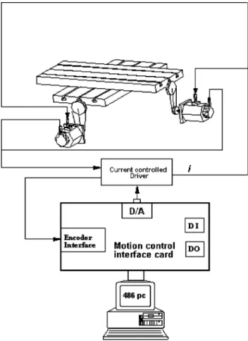
A retrofitted milling machine is used to test the track-ing performance of our proposed controller. The motion system shown in Fig. 7 comprises two torque-mode feed drives, 2:1 timing belts and pulleys, ball-screws and guide-ways, a motion card and a personal computer. This experimental servo system is built up in a so-called semi-closed loop, i.e., feedback signal is from the enco-der of servomotor. We use a PI velocity controller to handle the velocity loop control and a proportional gain in the position loop. The system modeling, identification and multiple loop design followed the previous work by the authors [14]. Both the simulation and experiment are performed to validate the proposed design. Two CCC designs are given for comparison, i.e.,

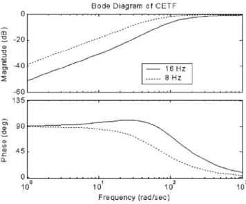
CCC1:x⫽ 1, wn⫽ 16 Hz (about 1/3 wvel)

CCC2:x⫽ 1, wn⫽ 8 Hz (about 1/6 wvel)

The corresponding Bode plots of CETF having high-pass characteristics for these two designs are shown in Fig. 8. It is clear from this figure that the wider the cut-off frequency of CETF is, the better attenuation of con-tour error can be achieved at low frequency. However, a wider cut-off frequency of CETF also corresponds to

Fig. 8. The Bode diagram of CETF.

a larger gain and a wider corner frequency of this PI-type cross-coupling controller, which may magnify the measurement noise. To compromise the effect of cross-coupling control and the influence of measurement noise, the cut-off frequency, or the stop band, of the CETF is chosen the same as bandwidth of the position loop.

Since the axial tracking controller is designed follow-ing the rule of multi-loop cascade control, there is nearly no servo mismatched between the two axes. No contour error for linear contouring motion will exist. Therefore, in the following discussions, we will focus on the circu-lar contour. For comparison, the results of simulations or experiments for three different cases are shown in one figure, where ‘1’ represents result of contour motion without CCC compensation and, ‘2’ and ‘3’ denote the results of contour motion with CCC1 and CCC2, respectively.

5.1. Circular motion with large radius

Two cases are conducted for comparison. The resol-ution of encoder is used as the basic unit length (BLU).

(1) R⫽ 50 mm (2×105_{BLU), Feedrate}⫽ 2.64 m/min

(circular frequency ⫽ 0.14 Hz)

(2) R⫽ 50 mm (2×105_{BLU), Feedrate}⫽ 7.5 m/min

(circular frequency ⫽ 0.4 Hz)

In the simulation and experimental studies, the refer-ence commands pass through an acceleration/deceleration (Acc/Dec) mechanism [15] before fed into the servo loop. This Acc/Dec mechanism can provide a smooth motion profile to avoid undesirable vibration. But it will also induce contour error during transient periods at the initial and final moments. Once the transient response dies out, the proposed method generates very good results.

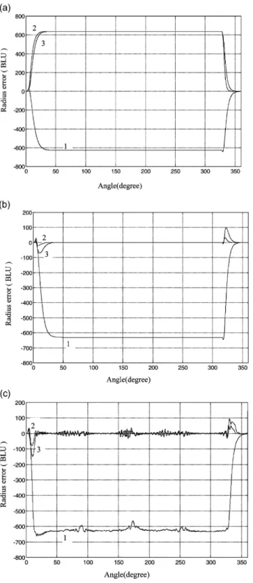
In case (1), since the tracking error is much smaller than the radius (the tracking error is about 3% of the radius), we obtain similar results by using the Eq. (1) or Eq. (4) in contour errors calculation. The simulation and experimental results in Fig. 9 confirm this point. How-ever, the increase of feedrate will degrade the perform-ance when Eq. (1) is used to estimate contour error, such as in case (2) where the tracking error is about 8% of the radius. The CCC needs a more accurate estimate of contour error obtained from Eq. (4) to perform the con-tour control. Fig. 10a shows that using Eq. (1) does not give the convergence of contour error, whereas using Eq. (4) does as shown in Fig. 10b. The experimental results are presented in Fig. 10c.

5.2. Circular motion with small radius

There are two cases for this comparison,

(3) R⫽ 2.5 mm (1×104_{BLU), Feedrate}⫽ 0.75

mm/min (circular frequency⫽ 0.8 Hz)

Fig. 9. Results of case (1): (a) Result of simulation, (b) Result of experiment.

Fig. 10. Results of case (2): (a) simulation with Eq. (1), (b) simul-ation with Eq. (4), (c) experiment with Eq. (4).

(4) R⫽ 2.5 mm (1×104_{BLU), Feedrate}⫽ 3 mm/min

(circular frequency ⫽ 3.2 Hz)

In case (3), since the tracking error is not very small when compared with the radius (the tracking error is about 16% of the radius), we use Eq. (4) in calculating

the contour errors. The simulation and experimental results are shown in Fig. 11. When the feedrate is increased such as in case (4), the tracking error becomes about 53% of the radius. The results shown in Fig. 12 demonstrated the effectiveness of our proposed design.

6. Conclusion

Combined with multiple-loop cascaded control design method, a new CCC structure with compensation at its reference position command is presented here, so is its stability analysis. Since the new structure allows the CCC to directly compensate the reference position com-mands of both axes, it has the potential to be integrated into any kind of axial tracking controller. In this paper, a simple proportional position-loop controller is used to demonstrate the feasibility of this kind of integration. The concept of contour error transfer function is adopted and the pole-placement method is used to design a PI-type CCC compensator. If a more sophisticated

Fig. 12. Results of case (4): (a) simulation, (b) experiment.

ler is employed in the position loop to improve single axial positioning accuracy or measurement noise is much concerned, Q(z⫺1) in Cc should be further shaped such

as adding more poles. Simulation and experimental results of our study both show that this dual-axis motion control system can achieve satisfactory contouring accu-racy under different motion conditions, such as large feedrate or small radius of curvature cases. Although it is not shown in this paper for general nonlinear path, Eq. (4) still valid if (R,q) are calculated on line, since

an arc can approximate nonlinear path locally. This new controller can be easily implemented on a majority of motion systems in use today via reprogramming the ref-erence position command subroutine only without any change in hardware of the motion systems.

Acknowledegments

The authors would like to thank the National Science Council of the Republic of China for financial support

of this manuscript under Contract No. NSC 89-2212-E-009-060

Appendix A

Discussion of a PI Controller as a Permissible Controller for CCC

Without loss of the generality, the discussion in this appendix is performed on S-domain. However, the implementation in the context is performed in discrete time or Z-domain. In the following, we will discuss the requirement and conditions forCc(s), F(s) and P(s) and

show that PI controller is a permissible cross-coupling controller.

The frequencies of contours under control are within the low frequency range as compared with the bandwidth of the servo system. In order to reduce the steady-state contour error or those low frequency components, the contour error transfer function (CETF), or 1

1⫹ CcP

, is required to have a very low gain at low frequency range, which amounts to requiring |CcP| be maximum at low

frequency range. Rewrite the CETF function in S-domain, we obtain

F(s)⫽ 1

1⫹ Cc(s)P(s)

. (A1)

The corresponding Bode plot of CETF will have high pass characteristics, i.e., F(0)→0. From Eq. (A1), we obtain Eq. (A2) as

F(s)⫹ F(s)·Cc(s)·P(s)⫽ 1 (A2)

and the conditions at low and high frequencies will be

F(0)⫹ F(0)·Cc(0)·P(0)⫽ 1 (A3a)

F(⬁) ⫹ F(⬁)·Cc(⬁)·P(⬁) ⫽ 1 (A3b)

The plant P(s) is user-designed and has low-pass charac-teristics, or,

P(0)⫽ const (A4a)

P(⬁) → 0 (A4b)

Because the compensator Cc(s) directly handles data

including possible measurement errors, it should have low gain at high frequency to avoid amplifying the high frequency noise. And from the viewpoint of implemen-tation, Cc(s)should be a proper or bi-proper function and

thus Cc(⬁) is finite. Substitute these known conditions

and apply them to Eq. (A3), we obtain the following equations easily,

F(⬁) ⫽ 1 (A5b) and

Cc(0)→⬁ (A6a)

Cc(⬁) is finite (A6b)

F(⬁) ⫽ 1 implies that F(s) is a bi-proper function,

other-wise, F(s) will diverge as s→⬁. From Eq. (A1), Cc(s)

can be represented as Cc(s)⫽ 1⫺F(s) F(s)·P(s) ⫽ 1⫺Nf(s) Df(s) Nf(s) Ff(s) ·Np(s) Dp(s) (A7) ⫽Dp(s)·(Df(s)⫺Nf(s)) Nf(s)·Np(s) ⫽(Df(s)⫺Nf(s)) Nf(s) ·P⫺1(s) where F(s)⫽Nf(s) Df(s) and P(s)⫽ Np(s) Dp(s), and Nf(s), Df(s),

NP(s) and Dp(s) are polynomials. Cc(s) is required to be

stable, thus, NP(s)and Nf(s) should not have roots with

positive real portions; that is, both F(s) and P(s) are of non-minimum phase. Also, since F(s) is a bi-proper function and F(⬁) ⫽ 1, the relative degree of Df(s)⫺Nf(s)

Nf(s)

will be at least one, and generally be one. From Eq. (A7), the relative degree of P(s) will be required to be one or less. It is true in our case, since P(s) is designed by cascade control to be a first order system. When P(s) is determined and fixed, we can see from Eq. (A1) that the cut-off frequency of F(s) is related to the magnitude of Cc(s) at that frequency. In theory, the

larger the cut-off frequency of F(s) is, the better per-formance the CCC system has. But a larger one will cause the design of the magnitude of Cc(s) becomes

larger at corresponding larger cut-off frequency. It will induce noise problem and degrade the performance of the system. To compromise the control effect of cross-coupling controller with the influence of measurement noise, the cut-off frequency, or the stop band, of the CETF is suggested to be the same as bandwidth of the position loop.

The simplest controller Cc(s) that matches above

requirements is a pure I controller. In this paper, a PI

controller is chosen as the CCC compensator for its ease on determining the transient response of the contour error correction. Other forms of controller are possible if the constraints of Eqs. (A5) and (A6) are satisfied.

References

[1] O. Masory, Improving contouring accuracy of nc/cnc systems with additional velocity feed forward loop, ASME Journal of Engineering for Industry 108 (1986) 227–230.

[2] M. Tomizuka, Zero phase error tracking algorithm for digital con-trol, ASME Journal Of Dynamic System, Measurement, and Con-trol 109 (1987) 65–68.

[3] Y. Koren, C.C. Lo, Variable-gain cross-coupling controller for contouring, Annals of the CIRP 40 (1) (1991) 371–374. [4] Y. Koren, Cross-coupled biaxial computer control for

manufac-ture systems, ASME Journal Of Dynamic System, Measurement, and Control 102 (1980) 265–272.

[5] P.K. Kulkarni, K. Srinivasan, Optimal contouring control of multi-axial feed drive servomechanisms, ASME Journal Of Dynamic System, Measurement, and Control 111 (1989) 140– 147.

[6] H.Y. Chung, C.H. Liu, A model-referenced adaptive control strat-egy for improving contour accuracy of multiaxis machine tools, IEEE Transaction on Industry Applications 28 (1992) 221–227. [7] Z.M Yeh., A cross-coupled bistage fuzzy logic controller for biaxis servomechanism control, Fuzzy Sets and Systems 97 (1998) 265–275.

[8] S.S. Yeh, P.L. Hsu, Theory and applications of the robust cross-coupled control design, ASME Journal of Dynamic System, Measurement, and Control 121 (1999) 524–530.

[9] K. Srinivasan, P.K. Kulkarni, Cross-coupled control of biaxial feed drive servomechanisms, ASME Journal of Dynamic System, Measurement and Control 112 (1990) 25–232.

[10] S.J. Huang, C.C. Chen, Application of self-tuning feed-forward and cross-coupling control in a retrofitted milling machine, Inter-national Journal of Machine Tools and Manufacture 35 (4) (1995) 577–591.

[11] F.B. Yeh, Post Modern Control Theory and Design, Eurasia Book Company, Taipei, Taiwan, 1990.

[12] G.C. Goodwin, S.F. Graebe, M.E. Salgado, Control System Design, Prentice-Hall, Englewood Cliffs, NJ, 2001.

[13] B.C. Kuo, Automatic Control Systems, Prentice-Hall, Englewood Cliffs, NJ, 1987.

[14] C.S. Chen, A.C. Lee, New direct velocity and acceleration feedf-orward tracking control in a retrofitted milling machine, Inter-national Journal of the Japan Society Precision Engineering 33 (3) (1999) 178–184.

[15] C.S. Chen, A.C. Lee, Design of acceleration/deceleration profiles in motion control based on digital FIR filters, International Jour-nal of Machine Tools and Manufacture 38 (1998) 799–825.