Narrow-Band Interference Suppression in
Spread-Spectrum CDMA Communications
Using Pipelined Recurrent Neural Networks
Po-Rong Chang,
Member, IEEE,and Jen-Tsung Hu
Abstract—This paper investigates the application of pipelined
recurrent neural networks (PRNN’s) to the narrow-band interfer-ence (NBI) suppression over spread-spectrum (SS) code-division multiple-access (CDMA) channels in the presence of additive white Gaussian noise (AWGN) plus non-Gaussian observation noise. Optimal detectors and receivers for such channels are no longer linear. A PRNN that consists of a number of simpler small-scale recurrent neural network (RNN) modules with less computational complexity is conducted to introduce best nonlin-ear approximation capability into the minimum mean-squared error nonlinear predictor model in order to accurately predict the NBI signal based on adaptive learning for each module from previous non-Gaussian observations. Once the prediction of the NBI signal is obtained, a resulting signal is computed by subtracting the estimate from the received signal. Thus, the effect of the NBI can be reduced. Moreover, since those modules of a PRNN can be performed simultaneously in a pipelined parallelism fashion, this would lead to a significant improvement in its total computational efficiency. Simulation results show that PRNN-based NBI rejection provides a superior signal-to-noise ratio (SNR) improvement relative to the conventional adaptive nonlinear approximate conditional mean (ACM) filters, especially when the channel statistics and exact number of CDMA users are not known to those receivers.
I. INTRODUCTION
S
PREAD-SPECTRUM communications are currently un-der development for wireless mobile communication ap-plications due to their efficient utilization of channel band-width, the relative insensitivity to multipath interference, and the potential for improved privacy [1]. In addition to providing multiple-accessing capabilities and multipath rejection, spread-spectrum (SS) communications also offer the possibility of further increasing overall-spectrum capacity by overlaying a code-division multiple-access (CDMA) network over narrow-band users [1]. CDMA is a promising technique for radio access in a variety of cellular mobile and wireless personal communication networks. In an SS-CDMA system, several independent users share simultaneously a common channel using spreading code waveforms. In addition, it offers some attractive features such as high flexibility, high capacity, simplified frequency planning, and soft capacity. For ex-ample, CDMA provides up to about four–six times more capacity than first-generation time-division multiple accessManuscript received August 5, 1996; revised December 27, 1996. P.-R. Chang is with the Department of Communication Engineer-ing, National Chiao-Tung University, Hsin-Chu, Taiwan (e-mail: pr-chang@cc.nctu.edu.tw).
J.-T. Hu is with AT&T.
Publisher Item Identifier S 0018-9545(99)00719-7.
(TDMA). Cellular systems, mobile satellite networks, and per-sonal communication networks (PCN’s) that use CDMA have been proposed and are currently under design, construction, or deployment [1]. Moreover, networks of low earth orbit (LEO) and medium earth orbit (MEO) satellites for worldwide (global) communications such as Loral/Qualcomm’s Glob-alstar and TWR’s Odyssey that employ CDMA have been developed [1].
The SS technique is inherently resistant to the narrow-band interference (NBI) caused by coexistence with conventional communications. However, it has been demonstrated that the performance of SS systems in the presence of narrow-band signals can be enhanced significantly through the use of active NBI suppression prior to despreading [2]–[14]. In a direct-sequence (DS) SS system, the transmitting spread signal is realized by modulating the signal with a pseudonoise (PN) sequence. At the receiver, the incoming signal is despread by correlating it with the same PN sequence. Thus, it is possible to reject interfering signals whose bandwidths are small compared to that of the spread signal. Moreover, since the spread signal has a nearly flat spectrum (white noise), it cannot be predicted from its past values. The interfering signal can be predicted accurately because it is narrowband. Once the prediction of the interference is obtained, an error signal is computed by subtracting the estimate from the received signal. Using the resulting error signal as the input to the correlator, the effect of the interfering signal can be reduced.
Since the direct-sequence SS signal can be modeled as an independent identically distributed (i.i.d.) binary sequence, such a sequence is highly non-Gaussian. Optimal detectors and receivers for predicting a narrow-band process in the presence of such a sequence are therefore no longer linear. Vijayan and Poor [11] proposed nonlinear methods of predicting the narrow-band signal that led to a significant increase in the signal-to-noise ratio (SNR) improvement due to filtering. This nonlinear method was derived from a system model that takes into account the non-Gaussian distribution of the observation noise. The observation noise consists of additive white Gauss-ian noise (AWGN) plus the SS data signal. Meanwhile, the NBI signal is modeled as an autoregressive (AR) process. Vijayan and Poor [11] applied a Masreliez-type approximate conditional mean (ACM) filter [13] to the AR process whose statistics are known to the receiver. The nonlinearity of ACM filter takes the form of soft-decision feedback of an estimate of the spread-spectrum signal. The performance of this approach
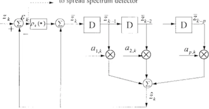
Fig. 1. Estimator/subtractor model for NBI rejection in SS-CDMA systems.
is significantly better than the linear Kalman filter. However, the problem with this approach is the difficulty of achieving the NBI rejection when the AR parameters are not known to the receiver. Therefore, Vijayan and Poor used the nonlinearity in the ACM filter to develop adaptive nonlinear LMS algorithms that do not need the AR parameters. Recently, Rusch and Poor [12] have proposed an adaptive ACM filter based on the residual less the soft-decision feedback in order to track the performance as well as the ACM filter did when the statistics are known. However, the performance of both adaptive ACM filters becomes worse when the exact number of CDMA users is not known to both filters. This is called the offset problem due to improper referencing of the nonlinearity caused by the number of users [12].
An alternative approach to the NBI rejection is based on neural networks. Bijjani and Das [15] applied the multilayered perceptron (MLP) neural network to NBI rejection in SS communications. However, MLP’s suffer from drawbacks of slow convergence and unpredictable solutions during learning. To overcome this difficulty, an alternative architecture to the prediction of an NBI signal with the flexibility to adapt to changing non-Gaussian environment is based on recurrent neu-ral networks (RNN’s) [16]. RNN is well suited for the adaptive prediction of a nonstationary nonlinear time series [17], [19]. Several algorithms have been proposed for the training of the RNN’s. The most widely known algorithm is the real-time re-current learning (RTRL) algorithm, proposed by Williams and Zipser [18], which can be used to update the synaptic weights of the RNN in real time. However, a sufficiently large number of neurons are required to maintain the prediction accuracy of the RNN-based predictor, but also increase its computational complexity. To tackle this difficulty, in Section III, a pipelined recurrent neural network (PRNN), proposed by Haykin and Li [20], is introduced to implement the adaptive nonlinear pre-dictor for NBI rejection with low computational complexity. Finally, in Section IV, we present an experimental study of the PRNN applied to the NBI rejection in SS-CDMA systems.
II. CONVENTIONAL NONLINEARTECHNIQUES FOR INTERFERENCE SUPPRESSION IN
MULTIPLE-USER SPREAD-SPECTRUM SYSTEMS A. Estimator/Subtractor Model for NBI Suppression
Fig. 1 illustrates a received signal that is passed through a filter matched to the chip waveform and chip-synchronously
sampled once during each chip interval. The equivalent dis-crete time received signal has three components due to the SS signal , the NBI , and the ambient white noise . The observation at sample is given by
(1) The ambient noise can be modeled as an AWGN with variance , the interference having bandwidth much less than the spread bandwidth, and the SS signal being the sum of independent, equiprobable, binary, and antipodal random variables and having the following binomial density function: (2)
where is the number of users in the SS-CDMA system. As noted in the preceding section, the three signals can be assumed to be mutually independent.
In this section, we describe nonlinear methods that offer improved NBI suppression capability over linear methods in the estimator/subtractor configuration of Fig. 1. This work was developed in [11]–[14]. The estimator/subtractor imple-mentation essentially forms a replica of the NBI which can be subtracted from the received signal to enhance the wide-band components. A method of producing such a replica is to exploit the disparity in the predictability of the NBI, i.e., and the SS signal, i.e., . In particular, the SS signal cannot be predicted from its past values since it has a nearly flat spectrum (white noise). Meanwhile, the interfering signal can be predicted accurately because it is narrowband. Hence, a prediction of the received signal using the estimating filter based on previously received values will, in effect, be an estimate of the interfering signal. In other words, the estimating filter removes the white-noise-like SS signal from the received signal. Thus, by subtracting predicted values of the received signal obtained in this way from the actual received signal and using the resulting prediction error as the input to the SS detector, i.e., PN correlator, the effect of the NBI can be reduced significantly. In addition, Vijayan and Poor [11] showed that the NBI can be modeled as a Gaussian autoregressive (AR) process of order , i.e.,
(3)
where is a white Gaussian process and are AR parameters.
From (1) and (3), a state-space representation for the re-ceived signal and the interference is given by
(4) (5) where
parameters given by
(6)
The observation noise in the state-space system ( ) is a sum of the white Gaussian measurement noise and the SS signal .
It is noted that the first component of the state vector is the interference . Hence, an estimate of the interference can be obtained by estimating the state from the received signal. Then, the interference rejection is performed by subtracting the estimate from the received signal. The estimate of based on observations until time is called the filtered estimate, and the estimate of based on observations until time is called the predicted estimate. It is known that the optimums of such estimates, in the mean-square error (MSE) sense, at time are the conditional means
and , where
denotes the set of observations recorded up to time . The optimal filtered and predicted estimates may be obtained from the Kalman–Bucy filtering equations when and are Gaussian processes. However, the observation noise is highly non-Gaussian [11]. For example, for a SS-CDMA system with a single user, the probability density function (pdf) of is a weighted sum of two Gaussian densities since is the sum of a Gaussian random variable and one that takes values of 1 with equal probability, i.e.,
(7) where is the zero-mean Gaussian probability density.
From (7), its expression shows that the pdf of is highly non-Gaussian. In [13], Masreliez developed an ACM filter to estimate the state of a linear system with non-Gaussian observation noise. Moreover, Vijayan and Poor [11] have applied the Masreliez concept to NBI rejection in SS-CDMA systems.
B. Approximate Conditional Mean (ACM) Filters for SS-CDMA Channels with Known Statistics
Assume that the AR parameters are constant and known to the receiver. Using the Masreliez assumption that the state prediction density is Gaussian with mean and covariance matrix , the optimal predicted estimate and its covariance can be recursively calculated as (8) (9) (10) (11) where (12) (13) and and denotes the observa-tion predicobserva-tion density.
Consider a system with one CDMA user. The pdf of observation noise is a Gaussian mixture of (7). Vijayan and Poor [11] have shown that the score function and its derivative are expressed as
(14) (15) where denotes the innovation signal and is its variance, that is,
(16) It can be seen that without the nonlinear terms tanh and sech, the ACM filter reduces to the Kalman–Bucy filter. From (14), the ACM filter provides decision feedback in the tanh, that is, it corrects the measurement by a factor in range that estimates the SS signal.
The previous systems with users have a very similar structure. In this case, the observation noise is a more compli-cated Gaussian mixture than that given in (7). The expression of the pdf of the current observation is in a form of Gaussian mixture, i.e.,
(17) According to (17), Rusch and Poor [12] have shown that the Masreliez nonlinearities can be derived as follows:
(18)
(19) where is given by
(20) Equation (18) is a smooth quantizer used to produce an estimate of the total SS signal. The nonlinearity in the smooth quantizer reduces to the tanh function when is unity. Moreover, the performance of the ACM filter will degrade as the number of users increases since the increased power of the SS signal causes the observation noise to be even more highly non-Gaussian when the filter employs the tanh term.
Fig. 2. Adaptive linear predictor.
C. Adaptive ACM Filters for SS-CDMA Channels Whose Statistics Are Unknown
In the previous section, the ACM filter performs appreciably better than the optimal linear Kalman filter when the AR parameters of the interference are known to the receiver. However, in practice, these AR parameters are random and not known to the receiver. Therefore, an effective suppression filter should be able to adapt itself to variations in the interference characteristics. In [8] and [9], Iltis, Li, and Milstein have applied simple linear transversal filters to the problem of NBI rejection. Fig. 2 illustrates the system diagram of a th-order linear filter. Their tap weights are adjusted using the Widrow LMS algorithm as follows:
(21) where is the estimated tap weight at time , denotes the obser-vation vector, is the prediction error or the residual of the prediction, and is a normalized step size. Note that is the predicted value of the received signal based on the immediate past values. Finally, the prediction error is sent to the SS detector, i.e., PN correlator. In order to both speed convergence and ensure the stability, the value of can be determined by
(22) where is chosen small enough to ensure the convergence and is an estimate of the input power, which is obtained by (23) and is a forgetting factor chosen to yield a compromise between the prediction accuracy and the tracking capability.
Unfortunately, the noise in this LMS algorithm is the observation noise which is the sum of Gaussian and non-Gaussian noise. This would severely degrade the performance of LMS-based interference rejection. Therefore, the nonlin-earilty derived from the ACM filter can be incorporated into this LMS structure and thereby substantially remove the SS signal from the adaptation process. Fig. 3 depicts this concept.
Fig. 3. Adaptive nonlinear ACM predictor.
The appropriate nonlinearity is given by
(24) Vijayan and Poor [11] developed an adaptive nonlinear LMS algorithm based on the ACM nonlinearity. Its tap-weight update equations can be expressed as
(25)
where ,
, the nonlinear prediction of is given by
(26) , and can be estimated by
(27) where is a sample estimate of the prediction error variance, which can be obtained by , and
is a forgetting factor with value between zero and one. Recently, Rusch and Poor [12] have proposed the second adaptive ACM filter structure based on the residual less the soft-decision feedback to improve the performance of the above-mentioned LMS-based ACM filter and provide better results. By altering the weight update equation of (25) to be based on the residual less the soft-decision feedback, the new update equation is written as
(28) Similarly, the outputs of both the adaptive ACM filters are the residual signals of their predictions, i.e., . The residual signal contains both the SS signal and an AWGN. After inputting the residual signal into the detector, it is possible to obtain the desired user data. Rusch and Poor [12] have shown that this new adaptive filter was able to track the interference as well as the ACM filter did when statistics are known.
Adaptive ACM filtering for the case of multiple CDMA users follows directly from the case of a single user. However, there is an offset problem present due to improper referencing of the nonlinearity in (24) since the receiver actually does not know the exact number of CDMA users in the system. As the number of CDMA users increases, the offset becomes larger. Then its performance will degrade when the number of users increases. To tackle this difficulty, the next section will present an alternative approach based on RNN’s which is able to provide the satisfactory results that are almost independent of the number of CDMA users.
III. NONLINEAR ADAPTIVE FILTERS FOR NBI SUPPRESSION USING PRNN’s
RNN’s are neural networks that have feedback. RNN’s are highly nonlinear dynamical systems which exhibit a rich and complex dynamical behavior. Moreover, RNN allows any neu-ron in the network to be connected to any other neuneu-ron in the network. They have been proven better than traditional signal processing methods in modeling and predicting nonlinear and chaotic time series [17]. Connor et al. [19] have indicated that RNN’s are well suited for the nonlinear prediction of nonlinear AR process. There are a number of types of recurrent networks that have been proposed by several researchers [16], [18]. In this paper, we are trying to apply the most widely known architecture proposed by Williams and Zipser [18] to time series prediction. A network with this particular architecture is also called the fully connected recurrent network.
Li [22] have shown that an RNN with a sufficiently large number of neurons and appropriate weights can be found by performing the real-time recurrent learning (RTRL) [18] algorithm such that the sum of the squared prediction errors for an arbitrary . In other words, , where denotes the norm with respect to the training
set , where and are the actual system and estimated RNN-based system model, respectively. Moreover, the RNN has the ability to generalize learning to what has never been seen [18]. This is called the generalization from learning. This is particularly useful for learning a NBI signal via a non-Gaussian SS-CDMA channel where observations may be incomplete, delayed, or partially available. Thus,
, where denotes the set union of and a set of data that is not belonging to and . The RTRL algorithm is capable of nonlinear adaptive prediction of nonstationary signals and does not require a priori knowledge of time dependence among the input data. However, a major limitation of the RTRL algorithm is that its computational complexity is proportional to , where is the total number of neurons in the network. Since a sufficiently large number of neurons are required to maintain the prediction accuracy of the RNN-based nonlinear predictor, it seems infeasible to achieve the RNN-based prediction within an acceptable small time interval. To tackle this difficulty, Haykin and Li [20] proposed a new RNN structure called the PRNN that is an extension of the conventional RTRL algorithm. The design of such a network is based on the principle of divide and conquer, that is, a complex RNN with a large number of
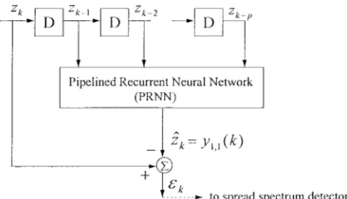
Fig. 4. Adaptive PRNN predictor.
neurons can be divided into a number of simpler small-scale RNN modules with less computational complexity. In the following section, we are trying to apply the PRNN structure to improve the computational performance of performing the nonlinear adaptive predictor. Fig. 4 shows the system diagram of PRNN-based nonlinear adaptive filter for NBI rejection. The PRNN-based filter is placed behind the channel and receives the channel output. The network inputs at time provides the desired response of the PRNN to train the network to achieve the optimal nonlinear adaptive filter by minimizing the prediction error (residual) . The estimate of actually contains a large portion of the NBI signal component since the other SS signal and AWGN components which have a flat spectrum cannot be predicted and are then filtered out by the PRNN-based filter. In other words, the predicted value of the received signal is, in effect, equal to the estimate of the NBI. Thus, by subtracting the estimate from the received signal, the residual signal becomes a sum of an AWGN and a SS signal. Once the optimal residual signal is obtained, the resulting prediction error signal is used as the input to the SS detector, i.e., PN correlator.
A. Low-Complexity PRNN’s
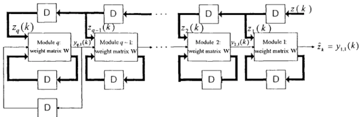
The PRNN shown in Fig. 5 is composed of identical modules, each of which is designed as a fully connected recurrent network with neurons. Each module has neuron outputs fed back to its input, and the remaining neuron output (the first neuron output) is applied directly to the next module. In the case of module , a one-unit delayed version of the module’s output is assumed to be fed back to the input. Information flow into and out of the modules proceeds in a synchronized fashion. Fig. 6 shows the detailed structure of module with neurons and external inputs. All the modules have exactly the same number of external inputs and internal feedback signals. Note that for module , its module output acts as an external feedback signal to itself. In addition, all the modules of PRNN are designed to have exactly the same ( -by- synaptic weight matrix . The updated value of the synaptic weight matrix is computed using the RTRL algorithm [18]. Haykin and Li [20] have demonstrated that the PRNN is able to provide the satisfactory accuracy of the nonlinear adaptive prediction of nonstationary signal and time series process. An important feature of the
Fig. 5. A PRNN with q modules.
Fig. 6. Detailed architecture of modulei of the PRNN.
PRNN is its high computational efficiency. Especially, the total computational requirement of processing a single sample on a PRNN is arithmetic operations. However, this is to be contrasted with computational requirement of a corresponding structure involving the use of a conventional RNN with neurons, that is arithmetic operations. Thus, the computational savings made possible by the use of PRNN can indeed be enormous for large .
For the th module, its external input at the th time point is described by the -by-1 vector
(29) where is the nonlinear prediction order. The other input vector applied to module is the -by- feedback vector
(30) where is the first neuron’s output in the adjacent module and denotes the internal feedback signal consisting of the one-step delayed output signals of neurons
in module and can be written as
(31)
Note that denotes feedback signals that originate from module itself. The last module of the PRNN, namely, module
, operates as a standard fully connected RNN. Thus, is written as
(32) Additionally, the fixed input 1 is included for the provision of a threshold applied to each neuron in module . Based on the above discussion, an input vector consisting of total input signals applied to module is represented (33) Thus, the th element of is represented by
(34) At the th time point, the output of neuron in module is computed by passing through a sigmoidal function , obtaining
(35) where the net internal activity is shown by
(36) Finally, the prediction computed by the PRNN at time instant is defined by the output of the visible (first) neuron of module 1 as shown by
(37) Note .
The main difference between the pipelined recurrent work of Fig. 5 and the conventional real-time recurrent net-work is that PRNN is characterized by a nested nonlinearity. Since all the neurons have a common nonlinear activation function , the functional dependence of the output
of the network in Fig. 5 on external inputs can be expressed as follows:
(38) where, for convenience of presentation, we have omitted the dependence on the synaptic weight matrix that is common to all the modules and . The expression of (38) is indeed the nested nonlinearity that gives the PRNN of Fig. 5 its enhanced computing power, compared to the conventional real-time recurrent network. Moreover, the scheme of nested nonlinear functions described in (38) is unusual in the classical approximation theory. Indeed, it is a universal approximator in the sense that a PRNN with appropriate training can approximate any nonlinear adaptive predictor to any desired degree of accuracy, provided that sufficiently many hidden neurons are available [22].
Certainly, is interpreted as the one-step prediction of computed by the th module whose functional de-pendence can be described by a complete dede-pendence form shown as follows:
(39) where is the synaptic weight matrix of module and is the input vector defined in (29) and (31). The desired response for module at time instant is . Hence, the prediction error for module is given by
(40) Note that for is the output residual signal sent to the SS detector. Thus, an overall cost function for the PRNN is defined by
(41) where is an exponential forgetting factor that lies in the range of . The inverse of is a measure of the memory of the PRNN. Adjustments to the synaptic weight matrix of each module is made to minimize in accordance with the real-time recurrent learning (RTRL) algorithm.
B. Real-Time Recurrent Learning (RTRL) Algorithm
For the case of a particular weight , its incremental change made at time according to the method of steepest descent is given by
(42)
where is the learning-rate parameter. From (39), (40), and (41), we note that
(43) In (43), the partial derivative is calculated using a modification of the RTRL algorithm [18]. A quadruply indexed set of variables is introduced to characterize the RTRL algorithm, and each element of the set is given by
(44) Note that . The RTRL algorithm is used to recursively compute the values of for every time step and all appropriate and as follows:
(45) with initial conditions
(46) where is a Kronecker delta equal to one when and zero otherwise, and and are defined in (34) and (36), respectively. From (35), we find that the derivative is given by
(47) Hence, it is possible to determine the value of at time instant by the recursion of (45) and (46). As a result, from (42), (43), and (44), the change applied to the ( )th element of the synaptic weight matrix is calculated by the following:
(48) The weight is updated in accordance with
(49) IV. SIMULATION RESULTS
Computer simulations have been carried out to compare the performance of PRNN-based, Kalman, ACM, adaptive linear, and two adaptive ACM interference rejection filters described above. The first adaptive ACM filter is the nonlinear prediction filter (NLP1) of (25) with the coefficients being updated using the LMS algorithm. The second adaptive ACM filter has the same nonlinear filter (NLP2) structure employing the residual less the soft-decision feedback of (28) with and . The number of filter taps is for each adaptive filter. The parameters of the proposed PRNN-based
Fig. 7. Comparison of mean square prediction errors achieved by PRNN predictor for AR interference with various numbers of users when input
SNR = 010 dB.
Fig. 8. Predictor performance for AR interference with known statis-tics—single CDMA user.
interference rejection filter were given by the following. The nonlinear prediction order is selected as four, the number of modules is chosen as five, the forgetting factor of (41) is set to 0.9, the learning rate is set to 0.001, and the number of neurons per module is chosen to two. The computational complexity of a weight-adjustment on the PRNN is on the order of , whereas the com-putational complexity of an adjustment on the conventional
Fig. 9. Predictor performance for AR interference with known statistics-multiple CDMA users.
recurrent network is on the order of . Thus, the PRNN reduces the computational complexity by more than two orders of magnitude. Moreover, by using a five-processor parallel computer, computational complexity per adjustment of PRNN is reduced to since each module is performed independently using its corresponding processor. To verify the rate of convergence for adaptive PRNN predictor, a performance index is in terms of the following mean square
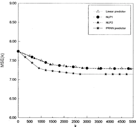
Fig. 10. Comparison of mean square prediction errors achieved by linear, NLP1, NLP2, and PRNN predictors for AR interference with 50 users when inputSNR = 010 dB and the number of users was not known to all the predictors.
prediction error given by:
MSE (50)
where denotes the prediction error at the th iteration for the th experiment (run) and is the total number of experiments (runs). Note that . Here, the value of
is chosen as ten.
Two kinds of NBI were considered in this paper: AR and si-nusoidal interference. We first considered the AR interference. The AR interfering signal was obtained by passing white noise through a second-order IIR filter with both poles at , i.e.,
(51) where is white Gaussian noise. The power of the back-ground thermal noise is kept constant at . The SNR at the filter input is defined as follows:
Input SNR (52) Fig. 7 depicts MSE convergence of PRNN predictor for AR interference with a various number of CDMA users when input SNR is equal to 10 dB relative to a unity power SS signal. From Fig. 7, it is seen that adaptation times were longer for a larger number of users. Moreover, since the prediction error contains the total SS signal, the steady-state value of the MSE prediction error is proportional to the number of SS-CDMA users. In order words, the steady-state MSE value increases as the number of users increases.
Next, a performance measure used to verify the interference rejection filters is the ratio of SNR at the output of the filter to the SNR at the input and given by
SNR improvement (53) where the SNR at the filter output is given by
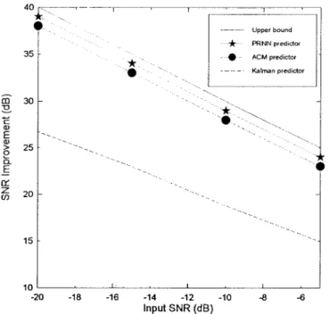
Output SNR (54) First, three filters were compared, namely, Kalman, ACM, and PRNN when Kalman and ACM filters knew the AR parameters and the exact number of CDMA users, whereas PRNN did not know these parameters. Figs. 8 and 9 show the comparison of SNR improvements achieved by Kalman, ACM, and PRNN for the case of single and multiple users, respectively, when input SNR was varied from 20 dB to 5 dB. All results were based on ten trials, and for each trial, the simulations were run for 1500 samples for 1 and 10 users, for 3000 samples for 25 users, and for 6000 samples for 50 users. From Fig. 9, it is seen that the SNR improvements of both PRNN and ACM were almost independent of the number of users and close to the upper bound. Moreover, the PRNN provides a little SNR improvement better than ACM. However, for the Kalman filter, its performance will degrade as the number of users increases. For the input SNR with a lower value, the received signal contains a larger portion of the NBI signal. As mentioned above, the NBI signal component is good for prediction. Thus, all the predictors achieve the better SNR improvement performance when the input SNR is at the low value. Otherwise, their performances become worse
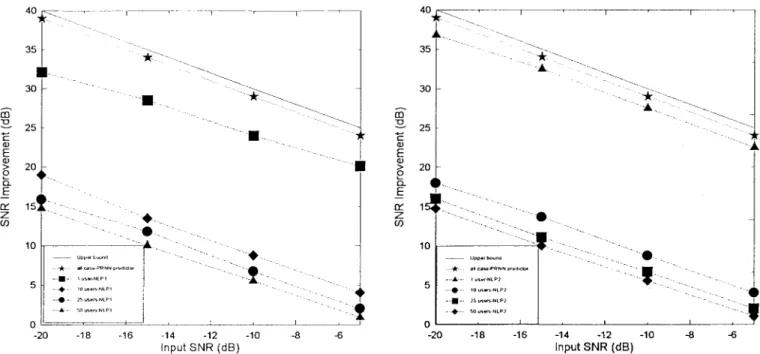
Fig. 11. Adaptive predictor performance for AR interference-multiple CDMA users when PRNN and NLP1 did not know the number of users.
as the input SNR increases. At the extreme case, there is no SNR improvement on each filter when received signal did not contain the interfering signal. In other words, each filter cannot offer the prediction capability for the white-noise-like received signal.
Next, four types of adaptive filters were compared, namely, linear, NLP1, NLP2, and PRNN when AR parameters and the number of users were not known to all the adaptive filters. Thus, both NLP1 and NLP2 employ the tanh term of (14) for a single user. Fig. 10 illustrates the MSE convergence of the four adaptive filters for AR interference with 50 users and input SNR dB. A comparison of the adaptation curves in Fig. 10 indicates that PRNN converges to the steady-state value much faster than the linear filter, NLP1, and NLP2. From Fig. 10, it is seen that both NLP1 and NLP2 performed as well as the linear LMS filter did because the tanh term in both NLP1 and NLP2 is not able to provide the sufficient nonlinear capability to deal with the high nonlinearity due to 50 users. Meanwhile, the PRNN with ten neurons is able to offer the accurate nonlinear prediction for dealing with the case of 50 users. For simplicity, Figs. 11 and 12 show the comparison of SNR improvements achieved by PRNN, NLP1, and NLP2 since the linear filter is always worse than the nonlinear filters and not considered in this case. It is seen that the SNR improvement of PRNN is independent of the number of users and almost coincides with the upper bound. Meanwhile, the performances of both NLP1 and NLP2 become worse as the number of users increases. However, once NLP1 and NLP2 know the exact number of users and employ the smooth quantizer of (24), their performances illustrated in Fig. 13 become better and are independent of the number of users. Especially, NLP2 was able to track the performance as well as the ACM filter did when the statistics were known. For this case, PRNN that did not know the exact number of users
Fig. 12. Adaptive predictor performance for AR interference-multiple CDMA users when PRNN and NLP2 did not know the number of users.
Fig. 13. Adaptive predictor performance for AR interference-multiple CDMA users when NLP1 and NLP2 knew the number of users.
still attains the better performance than that of both NLP1 and NLP2.
Another case we considered was a single-tone sinusoidal interference. The frequency of the sinusoidal interference signal was kept constant at 0.15 radians, i.e.,
(55) where is the amplitude and is a random phase with uniform distribution. It is shown that the performance is similar to that in the AR interference case. PRNN provides the better SNR improvement than that of all the other adaptive filters. Its performance almost coincides with the upper bound and is independent of the number of users.
V. CONCLUSION
This paper has introduced a new nonlinear NBI suppression technique based on PRNN which is capable of accurately predicting the NBI signal over the multiple-user SS-CDMA channel by using the RTRL learning algorithm. The PRNN-based predictor offers a superior SNR improvement perfor-mance to that of the conventional Kalman, ACM, and linear and nonlinear ACM adaptive filters because of its ability to approximate arbitrary nonlinear systems. For comparison of simulation results for both the AR and sinusoidal interfering signals, the SNR improvement of PRNN predictor with ten neurons and less computational complexity almost coincides with the upper bound and is independent of the number of CDMA users up to 50 users. However, the performances of all the conventional linear and nonlinear ACM adaptive filters become worse as the number of users increases when the number of users was not known to those adaptive filters.
REFERENCES
[1] A. J. Viterbi, CDMA, Principle of Spread Spectrum Communications. Reading, MA: Addison-Wesley, 1995.
[2] F. M. Hsu and A. A. Giordano, “Digital whitening techniques for im-proving spread-spectrum communications performance in the presence of narrow-band jamming and interference,” IEEE Trans. Commun., vol. COM-26, pp. 209–216, Feb. 1978.
[3] J. W. Ketchum and J. G. Proakis, “Adaptive algorithms for estimat-ing and suppressestimat-ing narrow-band interference in PN spread-spectrum systems,” IEEE Trans. Comm., vol. COM-30, pp. 913–924, May 1982. [4] L. M. Li and L. B. Milstein, “Rejection of narrow-band interference in PN spread-spectrum systems using transversal filters,” IEEE Trans.
Commun., vol. COM-30, pp. 925–928, May 1982.
[5] R. A. Iltis and L. B. Milstein, “Performance analysis of narrow-band interference rejection techniques in DS spread-spectrum systems,” IEEE
Trans. Commun., vol. COM-32, pp. 1169–1177, Nov. 1984.
[6] E. Masry, “Closed-form analytical results for the rejection of narrow-band interference in PN spread-spectrum systems—Part 1: Linear pre-diction filters,” IEEE Trans. Commun., vol. COM-32, pp. 888–896, Aug. 1984.
[7] , “Closed-form analytical results for the rejection of narrow-band interference in PN spread-spectrum systems—Part 2: Linear interpo-lation filters,” IEEE Trans. Commun., vol. COM-33, pp. 10–19, Jan. 1985.
[8] L. M. Li and L. B. Milstein, “Rejection of pulsed CW interference in PN spread-spectrum systems using complex adaptive filters,” IEEE Trans.
Commun., vol. COM-31, pp. 10–20. 1983.
[9] R. A. Iltis and L. B. Milstein, “An approximate statistical analysis of the Widrow LMS algorithm with application to narrow-band interference rejection,” IEEE Trans. Commun., vol. COM-33, pp. 121–130, Feb. 1985.
[10] E. Masry and L. B. Milstein, “Performance of DS spread spectrum receiver employing interference suppression filters under a worst-case jamming condition,” IEEE Trans. Commun., vol. COM-34, pp. 13–21, Jan. 1986.
[11] R. Vijayan and H. V. Poor, “Nonlinear techniques for interference suppression in spread-spectrum systems,” IEEE Trans. Commun., vol. 38, pp. 1060–1065, July 1990.
[12] L. A. Rusch and H. V. Poor, “Narrowband interference suppression in CDMA spread spectrum communications,” IEEE Trans. Commun., vol. 42, pp. 1969–1979, Apr. 1994.
[13] C. J. Masreliez, “Approximate non-Gaussian filtering with linear state and observation relations,” IEEE Trans. Automat. Contr., vol. AC-20, pp. 107–110, Feb. 1975.
[14] H. V. Poor and L. A. Rusch, “Narrowband interferenc suppression in spread spectrum CDMA,” IEEE Personal Communications, pp. 14–27, 1994.
[15] R. Bijjani and P. K. Das, “Rejection of narrowband interference in PN spread-spectrum systems using neural networks,” in IEEE Global
Telecommunications Conf., Dec. 1990, pp. 1037–1040.
[16] Special Issue on Dynamic Recurrent Networks, IEEE Trans. Neural
Networks, vol. 5, pp. 153–340, Mar. 1994.
[17] G. Kechriotis and E. Manolakos, “Using recurrent neural networks for nonlinear and chaotic signal processing,” in IEEE Int. Conf. Acoustics,
Speech and Signal Proc., Apr. 1993, pp. 465–469.
[18] R. T. Williams and D. E. Zipser, “A learning algorithm for continually running fully recurrent neural networks,” Neural Computation, vol. 1, pp. 270–280, 1989.
[19] J. T. Connor, R. D. Martin, and L. E. Atlas, “Recurrent neural networks and robust time series prediction,” IEEE Trans. Neural Networks, vol. 5, pp. 240–254, Mar. 1994.
[20] S. Haykin and L. Li, “Nonlinear adaptive prediction of nonstationary signals,” IEEE Trans. Signal Processing, vol. 43, pp. 526–535, Feb. 1995.
[21] L. Li and S. Haykin, “A cascaded recurrent neural networks for real-time nonlinear adaptive filtering,” in IEEE Int. Conf. Neural Networks, San Francisco, CA, 1993, pp. 857–862.
[22] L. K. Li, “Approximation theory and recurrent networks,” in Int. Joint
Conf. Neural Networks, Baltimore, MD, 1992, vol. 2, pp. 266–271.
Po-Rong Chang (M’87) received the B.S. degree in electrical engineering from the National Tsing-Hua University, Taiwan, R.O.C., in 1980, the M.S. degree in telecommunication engineering from Na-tional Chiao-Tung University, Hsinchu, Taiwan, in 1982, and the Ph.D. degree in electrical engineering from Purdue University, West Lafayette, IN, in 1988.
From 1982 to 1984, he was a Lecturer in the Chi-nese Air Force Telecommunication and Electronics School for his two-year military service. From 1984 to 1985, he was an Instructor of Electrical Engineering at the National Taiwan Institute of Technology, Taipei, Taiwan. From 1989 to 1990, he was a Project Leader in charge of the SPARC chip design team at ERSO, Industrial Technology and Research Institute, Chu-Tung, Taiwan. Currently, he is a Professor of Communication Engineering at National Chaio-Tung University. His current interests include fuzzy neural networks, wireless multimedia systems, and virtual reality.
Jen-Tsung Hu received the B.S. and M.S. degrees in communication engineering from National Chiao-Tung University, Hsinchu, Taiwan, R.O.C., in 1995 and 1996, respectively.