Jump Distribution Characteristics: Evidence from European Stock Markets

全文

(1)International Journal of Business and Economics, 2010, Vol. 9, No. 1, 1-22. Jump Distribution Characteristics: Evidence from European Stock Markets Thierry Ané* Finance Department, University of Reims, France Carole Métais DRM Finance, University Paris Dauphine, France. Abstract A comparison of the realized variance and the realized bipower variation provides a nonparametric estimation of the sum of all the intraday squared jump sizes. To recover individual jumps from this overall contribution to the quadratic variation, one needs to estimate both the number of jumps per day and their respective size. We provide a framework to do so and analyze the unconditional distributional properties of the two components of a jump – intensity and size – for three leading European stock market indexes. Key words: realized volatility; jumps; bipower variation; stock market indexes JEL classification: C14; C51; G11. 1. Introduction Since the origins of modern finance, continuous-time diffusion processes have played a central role in financial modeling, allowing one to elegantly solve problems as important as the pricing and hedging of derivative products. However, the recent availability of high-frequency data for a wide range of financial assets makes it now possible to zoom into an asset price evolution at a scale fine enough to sometimes observe price changes that are too sharp over too small time intervals for them to remain compatible with a pure diffusion process. Consequently, in recent years, there has been a growing interest toward modeling discontinuities in asset returns, the so-called jumps, caused by large informational shocks or extreme events. The explicit incorporation of jumps in the price process is not new and can be traced back to Merton (1976). This literature, however, remains essentially parametric with all the subjectivity this implies. In this context, the accuracy of empirical findings. Received June 1, 2009, revised March 31, 2010, accepted April 11, 2010. * Correspondence to: University of Reims, 57bis rue Pierre Taittinger, 51096 Reims Cedex, France. E-mail: ane@planete.net..

(2) 2. International Journal of Business and Economics. thus critically depends on the relevance of the assumed models. Whatever the specifications of the jump-diffusion process, however, probability theory teaches us that the quadratic variation can be divided into a smooth systematic component and a jump component. Building on this simple observation and with the help of a powerful asymptotic theory, Barndorff-Nielsen and Shephard (2004, 2006a, and 2006b) develop strong econometric devices for detecting the presence of jumps in a fully nonparametric setting. Their key idea is to compare two measures of price variability: the realized variance introduced in Andersen, Bollerslev, Diebold, and Ebens (2001) and Andersen, Bollerslev, Diebold, and Labys (2001), which includes the contribution of jumps, if any, as it approximates the quadratic variation, and the so-called bipower variation, constructed from the summation of appropriately scaled cross-products of adjacent high-frequency absolute returns, which happens to be robust to the jump contribution and only approximates the smooth component of the quadratic variation. It becomes therefore possible, at least in theory, to identify the occurrence of jumps by testing the significance of the difference between these two measures. This article builds on their ingenious theoretical results. The ability to separate the jump component from the smooth component of price variations remains insufficient, however, to allow for a comprehensive study of jump distribution characteristics. Indeed, the comparison of the realized variance and bipower variation simply yields the daily part of the quadratic variation attributable to jumps, that is, the sum of all intraday squared jump sizes. In order to go back from this daily contribution to the individual jumps one needs to estimate both the number of jumps per day and their individual sizes, including the sign or direction of the jump hidden in the squared jump size. Andersen, Bollerslev, Frederiksen, and Nielsen (2007) introduce an algorithm based on Barndorff-Nielsen and Shephard’s (2004, 2006a, and 2006b) work to extract the number of jumps per day. The main contribution of this article is to offer a new way of splitting the daily contribution of jumps to the quadratic variation and relate it to individual intraday discontinuities. The knowledge of the number of daily jumps and their sizes and directions thus allows one to analyze their distributional characteristics in a nonparametric framework. Using an intraday database on the three leading European stock indexes, we then provide a thorough investigation of the jump process with a special emphasis on the distributional characteristics of both the jump intensity and size. In summary, we observe that for all indexes the estimated jump intensity is sufficiently high to safely reject a purely diffusive process. Jumps tend to remain isolated events and days with more than one jump appear to be marginal. Finally, the classically used Poisson distribution seems to describe correctly the unconditional jump arrival process. Regarding the magnitude of discontinuities, since many asymmetries are observed between the positive and negative jumps in all markets, upward and downward discontinuities benefit from separate modeling. After trying several distributions already discussed in financial applications, we find that the Extended Burr XII density may be flexible enough to describe all jump series. We thus.

(3) 3. Thierry Ané and Carole Métais. conclude that the unconditional jump sizes could possibly be modeled by a mixture of Extended Burr XII distributions. However, we also note that our final model for the jump process could be improved with the use of time-varying parameters since serial dependence is observed in both the jump intensity and jump size series. The remainder of this paper is organized as follows. Section 2 presents the theoretical framework underlying our jump detection method. Section 3 describes the data together with a preliminary analysis. Section 4 introduces the algorithm used to extract individual intraday jumps. Section 5 focuses on empirical analysis of the jump process, first gathering our findings on the jump intensity then documenting evidence about jump size. Section 6 contains concluding remarks. 2. Jump Detection Method Let us first consider a continuous-time jump-diffusion process for the logarithmic price p(t ) of a financial asset. It is conveniently expressed in stochastic differential equation form as: dp (t ) = μ (t )dt + σ (t )dW (t ) + k (t )dq (t ) .. (1). The drift μ (t ) is generally supposed to be a continuous process with locally bounded variations while the volatility σ (t ) is simply assumed to be a nonnegative càdlàg process to allow for occasional jumps. W (t ) denotes a standard Brownian motion and k (t )dq (t ) represents a pure jump process that can be decomposed into a counting process q(t ) with (possible) time-varying intensity λ (t ) and the jump size, characterized by k (t ) = p (t ) − p(t − ) with the usual notation − p(t ) = lim s ↑t p ( s ) . If we denote by R(t ) = p(t ) − p (0) the logarithmic return over the time interval [0, t ] , it is well-known from the theory of quadratic variation that: [ R, R]t = ∫ 0 σ 2 ( s )ds + ∑ 0≤ s ≤t k 2 ( s ) , t. (2). where the first term on the right corresponds to the integrated variance of the continuous sample path component in (1) while the second term represents the sum of the q(t ) squared jump sizes observed between 0 and t . As a starting point for the analysis let us now assume that time t is measured in daily units and for any day t = 1,K , T , we define the j th intraday δ -period logarithmic return as: Rt , j (δ ) = p (t − 1 + jδ ) − p(t − 1( j − 1)δ ) ,. (3). where 1 δ is the sampling frequency and j = 1,K ,1 δ (to simplify notation, and without loss of generality, we assume that 1 δ is an integer). The nonparametric jump detection technique used in this article relies on the direct comparison of two estimates of the asset variability. On the one hand, Andersen, Bollerslev, Diebold,.

(4) 4. International Journal of Business and Economics. and Ebens (2001) and Andersen, Bollerslev, Diebold, and Labys (2001) sum the 1 δ squared intraday returns to obtain the so-called daily realized variance: RVt (δ ) = ∑ j =1 Rt2, j (δ ) . 1δ. (4). On the other hand, Barndorff-Nielsen and Shephard (2004) introduce the bipower variation: BVt (δ ) = μ1−2 (1 − 2δ ) −1 ∑ j =3 Rt , j (δ ) Rt , j −2 (δ ) , 1δ. (5). obtained as the sum of multiplied absolute intraday returns where μ1 = E Z = 2 π represents the mean of the absolute value of a standard Gaussian variable Z . As the sampling frequency of the underlying returns increases (i.e., as δ → 0 ), it can be shown that: RVt (δ ) → ∫t −1 σ 2 ( s )ds + ∑t −1< s≤t k 2 ( s ) , t. (6). while BVt (δ ) → ∫t −1 σ 2 ( s )ds . t. (7). Hence, the fundamental difference between the two measures is that while the realized variance estimator encompasses both variation due to the diffusive and the jump components, the realized bipower variation remains robust to discontinuities in the price movements.1 It is thus possible in theory to obtain a consistent nonparametric estimator of the jump contribution through the difference RVt (δ ) − BVt (δ ) . Due to sampling errors, however, this simple estimate of all squared intraday jump sizes ∑t −1< s≤t k 2 ( s ) may take a negative value or a nonzero small positive value on days without jumps. A reliable test statistic is thus required to ensure a correct separation of the diffusive and jump contributions from the quadratic variation. Andersen, Bollerslev, and Diebold (2007) introduce the tripower quarticity: TQt (δ ) = δ −1 μ 4−33 (1 − 4δ ) −1 ∑ j =5 Rt , j (δ ) 1δ. 43. 43. Rt , j −2 (δ ). 43. Rt , j − 4 (δ ). 43. ,. (8). gamma function, to where μ 4 3 = E Z = 2 2 3 Γ(7 6)Γ −1 (1 2) and Γ(⋅) is the t approximate the variance of the variance process ∫t −1 σ 4 ( s )ds . Using this jump-robust measure, Huang and Tauchen (2005) compare the finite sample performances of several possible test statistics in a Monte Carlo analysis and conclude that a test based on the following asymptotic result:.

(5) 5. Thierry Ané and Carole Métais Z t (δ ) =. δ −1 2 [ RVt (δ ) − BVt (δ )]RVt −1 (δ ) [[μ1−4 + 2μ1−2 − 5]Max(1, TQt (δ ) BVt −2 (δ ))]1 2 → N (0, 1). (9). posseses excellent finite sample properties. Following their approach, we denote by Φ α the critical value of a standard normal variable at confidence level α , and identify as “significant” jumps only those producing a value of the test-statistic Z t (δ ) in (9) larger than Φ α . Consequently, if we let I (⋅) denote the indicator function, the estimated jump component takes the form: J t ,α (δ ) = I ( Z t (δ ) > Φα ) × [ RVt (δ ) − BVt (δ ) ] ,. (10). while the continuous sample path contribution is redefined as follows: Ct ,α (δ ) = I ( Z t (δ ) ≤ Φα ) × RVt (δ ) + I ( Z t (δ ) > Φα ) × BVt (δ ) .. (11). Obviously, the definition of jumps now depends on the chosen confidence level, or, in other words, on what jump sizes are considered significant. Following the recommendation of Huang and Tauchen (2005) and the recent work of Andersen, Bollerslev, and Diebold (2007), we consider three confidence levels: α = 95%, 99%, 99.9% . Since the empirical results are qualitatively the same, we only present our findings with α = 99% to save some space. 3. Data and Preliminary Analysis. The empirical investigation focuses on the three leading European stock market indexes: the Cac 40, the Dax 30, and the Ftse 100. The raw database consists of tick-by-tick prices for the seven-year period ranging from September 11, 2000, to October 23, 2007. In order to strike a balance between information and bias when identifying the jumps, we follow much of the existing literature and opt for a 5-minute frequency to compute the realized variance and bipower variation. As suggested by Andersen et al. (2000), we use the volatility signature plot technique, that is, we graphically represent the average realized variance for different frequencies in order to check the adequateness of our choice. The plots (not shown) support 5-minute sampling. Indeed, a higher sampling frequency would induce spurious jumps due to market frictions, while a lower frequency would lead to poor sample properties of the test statistic derived in (9). In GMT time, all three markets are open from 8:00 am to 4:30 pm, resulting in 102 daily intervals. However, the French market presents a pre-closing session starting at 4:25 pm. Consequently, to avoid any spurious end-of-day effect on the variance series, we exclude the last five-minute trading interval for all markets. This gives a total of 101 intervals per trading day. For each day t , t = 1, K , T = 1767 , in the database we let j , j = 1, K ,1 δ = 101 , index the different 5-minute intraday intervals and calculate the realized daily variance according to (4), the realized bipower variation described in.

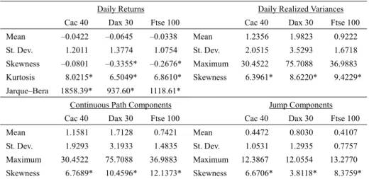
(6) 6. International Journal of Business and Economics. (5) as well as the continuous sample path component of (11), and the jump component according to (10). Table 1. Descriptive Statistics for Daily Returns, Realized Variances, and Their Constituents Daily Returns Mean St. Dev. Skewness Kurtosis Jarque–Bera. Daily Realized Variances. Cac 40. Dax 30. Ftse 100. –0.0422. –0.0645. –0.0338. 1.2011. 1.3774. 1.0754. –0.0801. –0.3355*. –0.2676*. Maximum. 6.5049*. 6.8610*. Skewness. 8.0215* 1858.39*. 937.60*. Cac 40. Dax 30. Mean. 1.2356. 1.9823. 0.9222. St. Dev.. 2.0515. 3.5293. 1.6718. 30.4522. 75.7088. 36.9883. 6.3961*. Dax 30. 8.6220*. 9.4229*. 1118.61*. Continuous Path Components Cac 40. Ftse 100. Jump Components. Ftse 100. Cac 40. Dax 30. Ftse 100. Mean. 1.1581. 1.7128. 0.7421. Mean. 0.4472. 0.8030. 0.4107. St. Dev.. 1.9293. 3.1933. 1.4835. St. Dev.. 1.0531. 1.2935. 0.7757. 30.4522. 75.7088. 36.9883. Maximum. 12.3867. 12.0554. 13.2770. 10.4596*. 12.1373*. Skewness. Maximum Skewness. 6.7689*. 6.6706*. 3.8118*. 8.3759*. Notes: * denotes significance at the 5% level.. Table 1 gathers the usual descriptive statistics for the daily returns as well as for the daily realized measures characterizing the variance and its continuous and jump components. Starting with the return series, one observes the usual characteristics to be expected from financial data: the presence of significantly fatter tails than those of a Gaussian distribution for all markets and a significant negative asymmetry for the Dax 30 and the Ftse 100. Not surprisingly, the Jarque-Bera test unambiguously rejects normality in all cases at the usual confidence level. Although the summary statistics do not reveal important distributional differences between the daily return series, they highlight heterogeneity in the realized variance behavior across markets. Average variance is twice as high in Germany as in the UK and its standard deviation also varies a lot from one market to another. The maximum daily variance observed in our sample and the skewness statistic reflect how much each realized variance series stretches to the right. The continuous sample path Ct , α (δ ) series is built, according to (11), by removing the jump component J t , α (δ ) from the realized variance. By construction, a jump component is located whenever the realized variance departs significantly from the bipower variation. One could assume that this may happen mainly for large observations of the realized variance and consequently expect the values of the continuous sample path component Ct , α (δ ) to extend much less to the right. Nevertheless, the skewness coefficients of the diffusive components displayed in Table 1 are slightly above the corresponding values for the realized variances. Moreover the maximum daily realized variance is the same as the maximum continuous path component for all three indexes. This could indicate that jumps are not necessarily associated with extreme volatility (even if this observation has to be.

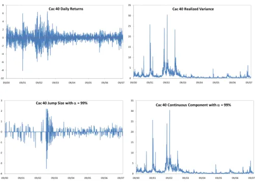
(7) 7. Thierry Ané and Carole Métais. taken with caution since, as pointed out by a referee, jumps are harder to identify on highly volatile days) and that a more straightforward method of extricating jumps from diffusive components with a threshold level on the variance would fail to identify the correct jump dates. Eventually, the statistics for the jump components indicate the existence of very different distributional properties of jump sizes in the three European markets. Figure 1. Returns, Variances, and Continuous and Jump Components for the Cac 40 8. 35. Cac 40 Daily Returns. Cac 40 Realized Variance. 6. 30. 4 25. 2 0. 20. ‐2. 15. ‐4 10. ‐6 5. ‐8. 0. ‐10 09/00. 09/01. 3. 09/02. 09/03. 09/04. 09/05. 09/06. 09/07. 09/00. 09/02. 09/03. 09/04. 09/05. 09/06. 09/07. 35. Cac 40 Jump Size with α = 99%. Cac 40 Continuous Component with α = 99%. 2. 30. 1. 25. 0. 20. ‐1. 15. ‐2. 10. ‐3. 5. ‐4 09/00. 09/01. 0 09/01. 09/02. 09/03. 09/04. 09/05. 09/06. 09/07. 09/00. 09/01. 09/02. 09/03. 09/04. 09/05. 09/06. 09/07. Additional insights about the realized variance and its constituents can be obtained with a visual representation of the reconstructed series. We plot in Figures 1, 2, and 3 the daily returns, realized variance, jump size, and continuous component for the Cac 40, Dax 30, and Ftse 100 respectively. The daily return graphs confirm the presence of heteroscedasticity with clusters of high and low variability periods. The realized variance estimates perfectly capture this stylized behavior and reveal a close correspondence between periods of large positive or negative returns and periods of extreme volatility. Moreover, the similarities between the graphs for the realized variance and the continuous component are striking for all markets. Finally, if we now turn our attention to the jump size graphs, several important characteristics are worth mentioning that are present in all three markets (although they are easier to observe with the Cac 40 due to the smaller number of jump dates). First, the jump magnitude varies a lot over time. Hence the variable k (t ) modeling the jump size should have time-varying parameters. Moreover, the existence of time aggregation in jump arrival dates is also evident from the graph. This means that the.

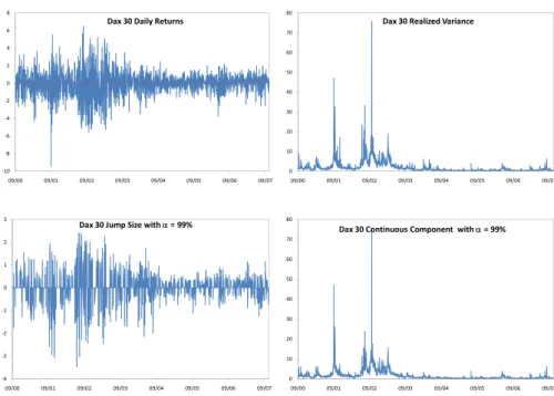
(8) 8. International Journal of Business and Economics. jump intensity λ (t ) for the counting process q(t ) would also need to be time-varying. In summary, both the size and intensity of the jump process seem to evolve over time and may require conditional modeling. Figure 2. Returns, Variances, and Continuous and Jump Components for the Dax 30 8. 80. Dax 30 Daily Returns. Dax 30 Realized Variance. 6. 70. 4. 60. 2 50 0 40 ‐2 30 ‐4 20. ‐6. 10. ‐8 ‐10 09/00. 0 09/01. 3. 09/02. 09/03. 09/04. 09/05. 09/06. 09/07. 09/00. 09/01. 09/02. 09/03. 09/04. 09/05. 09/06. 09/07. 09/06. 09/07. 80. Dax 30 Jump Size with α = 99%. Dax 30 Continuous Component with α = 99% 70. 2. 60. 1. 50 0 40 ‐1 30 ‐2. 20. ‐3. 10. ‐4 09/00. 0 09/01. 09/02. 09/03. 09/04. 09/05. 09/06. 09/07. 09/00. 09/01. 09/02. 09/03. 09/04. 09/05. To conclude this preliminary analysis, Table 2 documents the number of days when discontinuities are present, which provides a first approximation of the average jump intensity. One can observe that discontinuities are more than twice as frequent in the UK as they are in France. With respective average jump intensities of 0.44 and 0.17, these two markets experience jumps on average every 2.28 or 5.77 days. The German market presents an intermediate situation with jumps occurring on average every 2.98 days. Although the overall number of jumps directly depends on the threshold α used in the calculation of the critical value Φ α , the relatively high number of jumps in all markets presents strong evidence against the use of a purely continuous stochastic process for the dynamics of asset returns. Beyond the intensity of jump occurrences, an informative variable to look at is the proportion of the total variance RVt (δ ) that can be explained by the jumps J t ,α (δ ) . Table 2 also includes descriptive statistics for the contribution of jumps to the total variance as measured by this ratio. Interestingly, we observe that this measure is quite stable across indexes with an average jump contribution of roughly 1 3 and a standard deviation only between 10% and 15%. When they occur, jumps are thus an important part of the overall variance for the day and their maximum contribution can be as large as 87.71%..

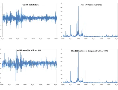
(9) 9. Thierry Ané and Carole Métais Figure 3. Returns, Variances, and Continuous and Jump Components for the Ftse 100 8. 40. Ftse 100 Daily Returns. Ftse 100 Realized Variance. 6. 35. 4. 30. 2 25 0 20 ‐2 15 ‐4 10. ‐6. 5. ‐8 ‐10 09/00. 0 09/01. 3. 09/02. 09/03. 09/04. 09/05. 09/06. 09/07. 09/00. 09/01. 40. Ftse 100 Jump Size with α = 99%. 09/02. 09/03. 09/04. 09/05. 09/06. 09/07. Ftse 100 Continuous Component with α = 99%. 35. 2. 30. 1. 25 0 20 ‐1 15 ‐2. 10. ‐3. 5. ‐4 09/00. 0 09/01. 09/02. 09/03. 09/04. 09/05. 09/06. 09/07. 09/00. 09/01. 09/02. 09/03. 09/04. 09/05. 09/06. 09/07. Table 2. Jump Intensity and Contribution to the Variability Cac 40 Number of Davs with Jumps. 306. Dax 30 593. Ftse 100 775. Proxy fro Jump Intensity. 0.1732. 0.3356. 0.4386. Average Jump Contribution. 0.2944. 0.3417. 0.3782. Standard Deviation of the Jump Contribution. 0.0985. 0.1288. 0.1461. Maximum Jump Contribution. 0.7177. 0.8255. 0.8771. Skewness of the Jump Contribution. 1.7125*. 1.2292*. 0.7863*. 4. From Global Jump Contribution to Individual Jumps. Despite all the interesting lessons one can draw from the analysis so far, our understanding of the jump process remains limited by the fact that, although we obtain the overall daily contribution of jumps to the quadratic variation, we are still unable to split it into individual jumps. Indeed, the comparison of the realized variance RVt (δ ) with the bipower variation BVt (δ ) through the test statistic Z t (δ ) simply allows one to obtain the quantity J t ,α (δ ) in (10), an approximation of ∑t −1< s≤t k 2 ( s ) , the daily part of the quadratic variation attributable to jumps. In.

(10) 10. International Journal of Business and Economics. order to provide a comprehensive analysis of the jump process, we need to estimate both the number of jumps per day q(t ) − q(t − 1) and their individual sizes k (s ) (including the sign) for s = t − 1 + jiδ , i = 1,K , q (t ) − q(t − 1) , t = 1,K , T = 1767 . To reach this goal, we now introduce the algorithm we apply to any day t in our sample. It is organized in two steps. The first determines the number of jumps per day q(t ) − q(t − 1) and their exact arrival times t −1 + jiδ for i = 1,K , q (t ) − q(t − 1) following the methodology introduced in Andersen, Bollerslev, Frederiksen, and Nielsen (2007). Here, in addition, the sign of each jump will be determined during this step. The second step focuses on the calculation of the absolute value of each jump size. We start the first step by calculating Z t (δ ) and compare it to the critical value Φ α . If the statistic is below the critical value, day t is considered to be exempt from jumps and q(t ) − q(t − 1) = 0 . Otherwise, at least one jump has occurred. To determine its arrival time we look for an intraday interval j1 such that: Rt2, j (δ ) = arg max j =1,K,1 δ =101 Rt2, j (δ ) .. (12). 1. We then consider that the largest jump in day t occurred during the interval [t − 1 + ( j1 − 1)δ , t − 1 + j1δ ] and assign it the time t − 1 + j1δ for notational simplicity. In addition to the discontinuity, the j1 th intraday return is made of a diffusive component. The two components of the return could have different directions. We assume, however, that when a jump occurs during an intraday interval, it represents a sufficiently large variation compared to the smooth component to dictate the resulting sign of the intraday return Rt , j1 (δ ) . This means that the jump direction can be determined as follows: sgn{ k (t − 1 + j1δ )} ≡ sgn{ Rt , j (δ )} ,. (13). 1. ⋅ denotes the sign function. where sgn{} Now that the first jump has been identified, we proceed to look for additional discontinuities for this day. Since the bipower variation in (5) is robust to the presence of jumps, this quantity will remain unchanged in the sequel. The realized variance, though, has to be recalculated to exclude the contribution of this first identified jump. To this point, a straightforward replacement could be obtained with 1δ the quantity ∑ j =1, j ≠ j Rt2, j (δ ) . Despite the simplicity, this is not advisable since for each new jump found the realized variance would be recalculated on one less squared return. This would introduce a downward bias in the realized variance relative to the bipower variation, resulting in an underestimation of the jumps with the statistic Z t (δ ) . To avoid this bias, we simply replace Rt2, j (δ ) by the average value of all the other intraday squared returns: 1. 1. R j2 ≡ (1 δ − 1) −1 ∑ j =1, 1δ. 1. j ≠ j1. Rt2, j (δ ) .. (14). The new realized variance filtered from the effect of the jump occurring in the j1 th interval in day t is thus estimated with:.

(11) 11. Thierry Ané and Carole Métais RVt (δ ) − j = ∑ j =1, 1δ. 1. j ≠ j1. Rt2, j (δ ) + R j2 .. (15). 1. With this value, we then calculate a new statistic Z t (δ ) − j according to (9) where the realized variance RVt (δ ) is simply replaced by RVt (δ ) − j . If this new statistic falls below Φ α , we consider that day t is characterized by the presence of a single jump ( q(t ) − q (t − 1) = 1 ) and move to the second step. Otherwise, we look again for arg max j =1,K,1 δ , j ≠ j Rt2, j (δ ) to identify the second largest jump in day t . We then proceed as before to calculate its sign sgn{k (t − 1 + j2δ )} ≡ sgn{Rt , j (δ )} and introduce a new statistic Z t (δ ) − j1 , − j2 to test for additional discontinuities. The procedure is repeated until the statistic Z t (δ ) − j1 ,K, − jq ( t ) drops below the critical value Φ α , indicate that no additional jumps are present for this particular day. With the number of jumps, their signs, and arrival times fully identified, we can proceed to the second step and calculate the last information required to recover each jump size: its absolute magnitude. To this end, recall that the quantity J t ,α (δ ) = RVt (δ ) − BVt (δ ) approximates the sum of all squared intraday jump sizes ∑t −1<s≤t k 2 ( s) . Hence, if a single jump has been found in day t , the summation reduces to a unique square term and the jump size is simply calculated by: 1. 1. 1. 2. k (t − 1 + j1δ ) ≡ sgn{Rt , j (δ )} × J t ,α (δ ) .. (16). 1. When multiple jumps have been detected in day t , however, one needs to assess their respective contributions to the daily jump component J t ,α (δ ) of the quadratic variation. We assume they can be obtained by looking at by how much each intraday squared return Rt2, j (δ ) , i = 1,K, q (t ) − q(t − 1) , contributes to the realized variance q (t ) calculated only on the intraday intervals exhibiting a jump, namely ∑i=1 Rt2, j (δ ) . The different jump sizes are thus computed with: i. i. k (t − 1 + jiδ ) ≡ sgn{Rt , j (δ )} × Rt2, j (δ ) i. i. ∑. q ( t ) − q ( t −1). i =1. Rt2, j (δ ) × J t ,α (δ ) ,. (17). i. for all i = 1,K, q (t ) − q(t − 1) . Note that the jump size definition in (17) guarantees q ( t ) − q ( t −1) 2 k (t − 1 + jiδ ) = J t , α (δ ) . The method adopted thus differs from that ∑i =1 Andersen, Bollerslev, Frederiksen, and Nielsen’s (2007) technique which sets the jump size equal to the corresponding intraday return Rt , ji (δ ) . Now that all the information for the jumps in day t has been extracted, the algorithm proceeds to the next day of the sample. 5. Empirical Analysis of the Jump Process 5.1 Number of Jumps and Jump Intensity. We apply the previously discussed algorithm to the three European stock index series and summarize in Table 3 the results relative to the number of daily jumps. The table first provides the count of the exact number of jumps between September 11, 2000, and October 23, 2007. The difference between the numbers of days with.

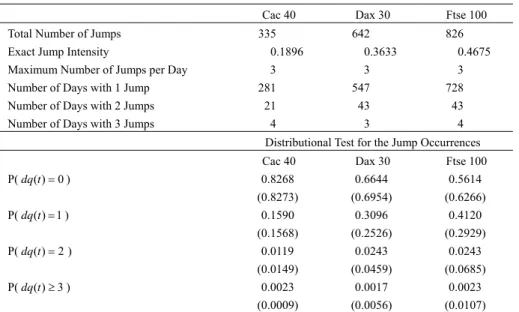
(12) 12. International Journal of Business and Economics. jumps reported in this table and those in Table 2 is due to the existence of days with more than one jump. With this exact jump count in hand, we can refine the approximation for the jump intensity in Table 2 by now dividing the number of jumps (and not the number of days with jumps) by the total number of days in our sample to form an estimate. Obviously, all jump intensities are increased. We then proceed to sort the jump days according to the number of jumps. For all indexes, more than 90% of jump days exhibit only a single jump, and there are no more than three jumps observed on any given trading day. This confirms that jumps are rare and represent isolated events. We note that the proportions of days with 1, 2, or 3 jumps (Table 4) are remarkably similar across markets. Table 3. Jump Arrival Times and Intensity Cac 40 Total Number of Jumps. 335. Dax 30. Ftse 100. 642. 826. Exact Jump Intensity. 0.1896. 0.3633. 0.4675. Maximum Number of Jumps per Day. 3. 3. 3. Number of Days with 1 Jump. 281. 547. 728. Number of Days with 2 Jumps. 21. 43. 43. Number of Days with 3 Jumps. 4. 3. 4. Distributional Test for the Jump Occurrences Cac 40. Dax 30. Ftse 100. P( dq (t ) = 0 ). 0.8268 (0.8273). 0.6644 (0.6954). 0.5614 (0.6266). P( dq (t ) = 1 ). 0.1590 (0.1568) 0.0119. 0.3096 (0.2526) 0.0243. 0.4120 (0.2929) 0.0243. P( dq (t ) = 2 ). (0.0149) (0.0459) (0.0685) 0.0023 0.0017 0.0023 (0.0009) (0.0056) (0.0107) Notes: In addition to the exact jump intensity for each stock index, this table provides the repartition of jumps per day. It also compares the empirical probabilities of the number of jumps per day to the classically used Poisson distribution. P( dq (t ) ≥ 3 ). At this point, recall that the daily jump contribution J t ,α (δ ) depends on the selected confidence level α and, consequently, so does the number of days exhibiting jumps. We want to test, however, the robustness of the algorithm introduced for the detection of the number of intraday jumps. To do so, we use our algorithm to calculate the number of days with 1, 2, 3, … jumps for α = 95%, 99%, 99.9% . We summarize the proportions obtained in Table 4. Mechanically, when the value of α is lowered, the overall number of jumps obtained increases. Consequently, one could expect a rise in the maximum number of jumps per day. The opposite effect is expected for a higher confidence level α . However, the empirical evidence in Table 4 reveals that the algorithm robustly estimates the number of days with multiple jumps. Indeed, when α = 95% the maximum number of jumps only rises to 4 and the proportions show that this little.

(13) 13. Thierry Ané and Carole Métais. increase only happens exceptionally, and when α = 99.9% the maximum number of jumps remains equal to 3. To ensure that the repartition of jump days according to the observed discontinuities is not statistically affected by a change in α , we nonparametrically test whether the proportion of days with 1, 2, 3, … jumps is different for the three possible values of α . For each index, we observe that there is no statistical difference in the percentage of days with multiple discontinuities (whether it is 2, 3, or 4). As expected, this result does not hold for the single-jump days since, in this case, the threshold α directly controls for the amount of noise-jumps. To conclude, the analysis of the results in Table 4 largely highlight the robustness of the number of jumps detection technique.2 Table 4. Robustness Analysis of the Number of Daily Jumps Detection Algorithm. Days with 1 Jump. α = 95% 0.8569≠≠ 0.8657≠≠ 0.8722≠≠. α = 99% α = 99.9% Cac 40 0.9183≠≠ 0.9530≠≠ ≠≠ Dax 30 0.9224 0.9587≠≠ ≠≠ Ftse 100 0.9394 0.9747≠≠ Days with 3 Jumps α = 95% α = 99% α = 99.9% Cac 40 0.0141 0.0131 0.0067 Dax 30 0.0200 0.0051 0.0026 Ftse 100 0.0124 0.0052 0.0018 Notes: ≠≠ denotes significance at the 5% level.. Days with 2 Jumps Cac 40 Dax 30 Ftse 100. Cac 40 Dax 30 Ftse 100. α = 95% 0.1254 0.1131 0.1124. α = 99% α = 99.9% 0.0686 0.0403 0.0725 0.0388 0.0555 0.0235 Days with 4 Jumps α = 95% α = 99% α = 99.9% 0.0035 0.0000 0.0000 0.0012 0.0000 0.0000 0.0031 0.0000 0.0000. Almost invariably, the parametric literature on jump-diffusion processes assumes a Poisson distribution for the counting process q (t ) in (1). Using the refined estimate for the jump intensity in Table 3, we calculate the theoretical probability of obtaining 0, 1, 2, or more jumps with a Poisson distribution and report these in parentheses below the corresponding empirical probability computed as the ratio of the number of days with 0, 1, 2, or more jumps over the total number of days. The pairs of probabilities are sufficiently close for all three European indexes to conclude that a Poisson distribution models reasonably well the probability of jump occurrences. Indeed, a researcher in search of an improvement in fit should not look for a better parametric distribution but simply focus on refining the definition of the jump intensity. As suggested by time aggregation in jump arrival dates (Figures 1, 2, and 3), the Poisson distribution would benefit from the introduction of a time-varying parameter. Explicitly modeling the time structure of all important quantities, however, is beyond the scope of this study, whose goal is purely to highlight how the essential components of a jump can be extracted nonparametrically and to present potential unconditional distributions..

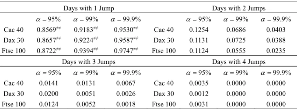
(14) 14. International Journal of Business and Economics Figure 4. Average Variability and Jump Repartition by Interval 0.10 0.09 . 0.2. Variability and Jump Repartition by Interval for the Cac 40. 0.18. 0.08 . 0.16. 0.07 . 0.14. 0.06 . 0.12. 0.05 . 0.1. 0.04 . 0.08. 0.03 . 0.06. 0.02 . 0.04. 0.01 . 0.02. 0.00 . 0. 0.10 0.14. Variability and Jump Repartition by Interval for the Dax 30. 0.09 0.08. 0.12. 0.07. 0.10. 0.06 0.08. 0.05 0.04. 0.06. 0.03. 0.04. 0.02 0.02. 0.01. 0.00. 0.00. 0.06. 0.06. Variability and Jump Repartition by Interval for the Ftse 100 0.05. 0.05. 0.04. 0.04. 0.03. 0.03. 0.02. 0.02. 0.01. 0.01. 0. 0. Notes: We use average squared returns per interval to highlight the intraday volatility pattern in the three cash index series (dotted lines) and superimpose these over the proportion of jump arrivals (histograms) by intraday interval to show its direct link with intraday volatility patterns..

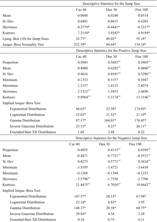
(15) Thierry Ané and Carole Métais. 15. Although the study of full conditional models is left for future research, there is still another type of seasonality worth discussing here: the intraday pattern in jump occurrences. As a byproduct of our jump detection procedure, we identify the intraday intervals j1 , K jq ( t )−q ( t −1) , where discontinuities are observed for a specific day t . Using this information we calculate the proportion of jumps occurring in each 5-minute interval. Figure 4 shows the histogram of jump arrivals for each stock market index. For the sake of comparison, we also compute the intraday seasonality T of the variance with T −1 ∑t =1 Rt2, j , j = 1, K ,1 δ , following Andersen and Bollerslev (1998). The obtained pattern is superimposed as a dotted line over the histogram. Strikingly, for all indexes, the variance and jump arrival time present the same inverted J-shaped pattern. Variance is high and jumps are much more frequent during the first five minutes of trading. Indeed, 20% of the Cac 40 jumps are concentrated there while this figure rises up to 58% or 76% for the Dax 30 and the Ftse 100 respectively. Volatility and jump arrivals then decline before experiencing two more peaks at 1:30 pm and 3:00 pm GMT. The initial peak can classically be explained by the pressure at a market opening after a long period of interrupted trading and the accompanying accumulated information. The remaining peaks, occurring at 8:30 am and 10:00 am in Eastern Standard Time, coincide with macroeconomic news announcements in the US. They thus suggest that a large proportion of the jumps observed in the European cash indexes are related to the release of regularly scheduled American news.3 5.2 Probabilistic Investigation of Jump Sizes. Now that the jump intensity has been studied, the next logical step is to turn our attention to the second component of a discontinuity, namely the jump size. The first part of Table 5 gives the usual descriptive statistics for the estimated jump sizes of the three European indexes. In all cases, the average jump size is not significantly different from zero, and the standard deviation is comparable in all markets. In the parametric literature on jump-diffusion processes, a normal distribution is generally assumed to characterize the magnitude of discontinuities, as in Eraker et al. (2003) and Duffie et al. (2000). Unfortunately, the significant asymmetry and excess kurtosis obtained for the three jump size series are obvious evidence against this distributional choice. The Jarque-Bera test unambiguously rejects the normality of jump sizes for the three markets. Even though we do not focus on conditional models in this article, we include in the first part of Table 5 a Ljung-Box test to investigate whether jump sizes are serially correlated. The values clearly indicate that small and large jump sizes are aggregated through time in the European markets. In agreement with our first intuition from Figures 1, 2, and 3, we can conclude that a conditional model would be required for the jump size. Hence both jump intensity and jump size seem to be time-varying..

(16) 16. International Journal of Business and Economics Table 5. Positive and Negative Jump Sizes. Descriptive Statistics for the Jump Size Cac 40. Dax 30. Ftse 100. Mean. 0.0048. 0.0240. 0.0314. St. Dev.. 0.6401. 0.8615. 0.6203. Skewness. –0.2779*. –0.4441*. –0.2317*. Kurtosis. 7.2158*. 3.9342*. Ljung–Box (10) for Jump Sizes Jarque–Bera Normality Test. 4.9194*. 32.71*. 49.02*. 55.18*. 252.39*. 44.44*. 134.18*. Descriptive Statistics for the Positive Jump Size Cac 40 Proportion Mean. Dax 30. Ftse 100. 0.5045. 0.5685≠≠. 0.5605≠≠. 0.4880. 0.6282. ≠≠. 0.4880≠≠. ≠≠. 0.3296≠≠. St. Dev.. 0.4016. 0.4541. Minimum. 0.1353. 0.1157. 0.1047. Maximum. 2.2157. 2.4123. 2.6074. Skewness. 2.5322≠≠. 1.5853. Kurtosis. 9.8984≠≠. 5.3174≠≠. 2.6696 13.1146≠≠. Implied Jarque–Bera Test: Exponential Distribution. 86.63*. Lognormal Distribution. 23.02*. 11.52*. 21.19*. Gamma Distribution. 87.17*. 164.01*. 176.45*. Inverse Gaussian Distribution. 25.13*. 8.21*. 26.11*. 1.68. 2.48. 0.22. Extended Burr XII Distribution. 32.58*. 174.85*. Descriptive Statistics for the Negative Jump Size Cac 40 Proportion Mean St. Dev.. Dax 30. Ftse 100. 0.4955. 0.4315≠≠. 0.4395≠≠. –0.4871. ≠≠. –0.5511≠≠. ≠≠. 0.3624≠≠. –0.7721. 0.4273. 0.5771. Minimum. –3.5195. –3.4721. –3.6438. Maximum. –0.1269. –0.1394. –0.1233. Skewness. –3.5796≠≠. –1.7558. –2.7706. Kurtosis. 21.4475≠≠. 6.7010≠≠. 18.6642≠≠. Implied Jarque–Bera Test: Exponential Distribution Lognormal Distribution Gamma Distribution Inverse Gaussian Distribution Extended Burr XII Distribution. 147.57*. 20.15*. 67.98*. 22.18*. 6.63*. 3.95. 148.37*. 20.38*. 68.75*. 29.84*. 4.34. 3.28. 0.18. 0.73. 0.11. Notes: * denotes significance at the 5% level and ≠≠ denotes that corresponding positive and negative quantities are statistically different in absolute value at the 5% level..

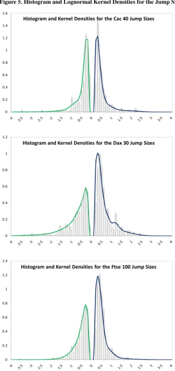
(17) Thierry Ané and Carole Métais. 17. Figure 5. Histogram and Lognormal Kernel Densities for the Jump Sizes 1.6. Histogram and Kernel Densities for the Cac 40 Jump Sizes 1.4 1.2 1 0.8 0.6 0.4 0.2 0. 1.2. Histogram and Kernel Densities for the Dax 30 Jump Sizes 1. 0.8. 0.6. 0.4. 0.2. 0. 1.4. Histogram and Kernel Densities for the Ftse 100 Jump Sizes 1.2. 1. 0.8. 0.6. 0.4. 0.2. 0. Since the classical Gaussian distribution cannot be used to describe the.

(18) 18. International Journal of Business and Economics. repartition of jump sizes, we need to look for an alternative parametric model. Even if it is not entirely accurate, a basic histogram could be useful to form an opinion about the shape of the jump size distribution and could help find a suitable model. Figure 5 presents this histogram for each stock index. One can observe that the mass around zero is very small, meaning that few small jumps are identified by our method. Indeed, as pointed out by a referee, whatever the jump detection technique one would opt for, the identification of small discontinuities is, theoretically and in practice, problematic. However, Zhang (2007) argues that one may assimilate small jumps to the diffusive part of the variance process and treat large jumps as a compound Poisson process without that being harmful to the analysis. In addition, we see that there is an important degree of asymmetry between the positive and negative sides. The last two subparts of Table 5 display the descriptive statistics of the jump sizes sorted by sign. First, we note that the proportion of positive and negative jumps is not significantly different for the Cac 40 whereas the other two indexes experience positive discontinuities more often (roughly 56% versus 44%). Similarly, no significant asymmetry in the average jump size or jump size standard error can be found on the French market. In Germany and the UK, however, negative jumps are more volatile and have a larger absolute magnitude on average. The maximum and minimum values as well as the skewness parameters confirm the existence of a strong asymmetry between the distribution of positive and negative discontinuities of all stock markets. Given the scarcity of theoretical distributions exhibiting these characteristics, we consider it best to separately model the negative and positive jump sizes (negative jump sizes will be modeled in absolute values below). To this point, to refine our perception of each jump size series (positive and negative for each index), it could be useful to obtain a nonparametric density estimate that is more robust that a simple histogram. A classical approach is to resort to a kernel density estimate. Traditional kernel methods are inappropriate here since they involve weights over the entire real line while the absolute jump sizes are bounded to the left by 0. Several solutions have been discussed in the abundant statistical literature on kernel density estimation. In order to maintain the simple spirit of the standard kernel estimators, we follow Chen’s (2000) recent approach and use asymmetric kernels of the form: N fˆ ( x; h) = N −1 ∑i =1 k ( x; a ( X i , h), b( X i , h)) ,. (18). where { X i }iN=1 represents a jump size series and a(⋅, h) and b(⋅, h) are two functions characterizing the shape parameters of the selected positive kernel K ( x; a(⋅ , h), b(⋅ , h)) with bandwidth parameter h . In this paper, the nonparametric density estimator is constructed with lognormal kernels of the form: K LN (u; α , β ) =. ⎧ (ln(u ) − α ) 2 ⎫ exp⎨− ⎬, 2β u 2πβ ⎭ ⎩ 1. (19).

(19) 19. Thierry Ané and Carole Métais with u > 0 and β > 0 . The lognormal kernel density estimator is then given by: N fˆ ( x; h) = N −1 ∑i=1 K LN ( x; ln( X i ), 4 ln(1 + h)) .. (20). We note that such lognormal kernel estimators achieve the optimal rate of convergence in the mean integrated square error within the class of nonnegative kernel density estimators. Moreover, the shape of the lognormal kernels varies naturally, which leads to the amount of smoothing being changed according to the position where the density estimation is made without explicitly changing the bandwidth. This implies that the lognormal kernel estimators in (20) are adaptive density estimators. Finally, the optimal bandwidth parameter is obtained by least square cross-validation. The obtained nonparametric densities are depicted in Figure 5 together with the previously discussed histograms. They will be used as a benchmark to assess the goodness-of-fit of the competing parametric distributions for the jump size. In the financial literature, when jumps are introduced in the volatility process and require a nonnegative distribution, the classical choice is an exponential model. Once again, this is how both Eraker et al. (2003) and Duffie et al. (2000) choose to describe the uncertainty in the jump magnitude. Among the other usual distributions with a positive support one could think of to represent the size of a jump, the lognormal, gamma, and inverse Gaussian densities have a long list of applications in finance. For each series of jump absolute magnitudes, we calibrate these four distributions and test their goodness-of-fit with an implied Jarque-Bera statistic (i.e., we transform the initial jump size series { X i }iN=1 into {Φ −1[ F ( X i ,ψˆ )]}iN=1 where F (⋅,ψˆ ) is the parametric cdf with parameter vector ψˆ obtained by maximum likelihood and perform a usual Jarque-Bera test to check the normality). The results of this investigation, reported in the second and third part of Table 5 under the heading “Implied Jarque-Bera,” indicate that none of these classical distributions is flexible enough to accurately describe the jump size behavior. With four parameters to increase the flexibility, the Extended Burr XII distribution is certainly less popular in finance but has proved particularly useful in other sciences to describe positive random variables in modeling problems surprisingly not far from financial concerns. To give a single example, Shao, Wong, Xia, and Ip (2004) promote its goodness-of-fit for the modeling of extremes in flood frequency analysis. The Extended Burr XII distribution is characterized by the cdf: FBurr. ⎧⎪1 − [1 − τλ−θ ( x − μ )θ ] 1τ ( x ; μ , λ , θ , τ ) = ⎨ XII ⎪⎩1 − exp(− λ−θ ( x − μ )θ ). τ ≠0 τ = 0.. (21). The support for x is 0 ≤ x < ∞ when τ ≤ 0 and 0 ≤ x < λτ −1 θ when τ > 0 . The location parameter μ and the first shape parameter τ belong to ℜ while the scale parameter λ and the second shape parameter θ are nonnegative. We also calibrate this parametric model to each jump size series and rely on the previously discussed implied Jarque-Bera test4 to assess its relevance for the.

(20) 20. International Journal of Business and Economics. magnitude of discontinuities. The statistics reported in Table 5 show the adequacy of this distribution for positive and negative jump sizes of all stock indexes. We thus recommend describing the variable k (⋅) ≡ Y characterizing the jump through a mixture of Extended Burr XII distributions of the type: fY ( y ) = p1 f Burr. XII. (− y ; μ1 , λ1 , θ1 , τ 1 ) I ( y < 0) + p2 f Burr. XII. ( y ; μ2 , λ2 , θ 2 , τ 2 ) I ( y ≥ 0) ,. (22). where i = 1 and i = 2 represent the negative and positive jump size of a particular index, respectively, and p1 = P (k (⋅) < 0) = 1 − p2 represents the probability of a downward jump. We have already noted that jump sizes seem to be time-varying; consequently an additional improvement could probably be obtained by allowing the distribution’s parameters to evolve through time. However, this issue is beyond the scope of the current article and we leave it for future research. 6. Conclusion. Merton (1976) noted that “since empirical studies of price series tend to show far too many outliers for a simple, constant-variance lognormal distribution, there is a ‘prima facie’ case for the existence of jumps.” The recent generalization of ultra high-frequency data allows a visual confirmation of this intuition. Indeed, simple graphs of price evolutions reveal the presence of changes that are too sharp for them to come from a purely diffusive process. However, until recently, the estimation difficulty of jump-diffusion models has limited their use in empirical studies. Building on the ideas at the origin of the so-called realized variance of Andersen, Bollerslev, Diebold, and Ebens (2001) and Andersen, Bollerslev, Diebold, and Labys (2001), Barndorff-Nielsen and Shephard (2004, 2006a, and 2006b) introduced a new variance estimate, called realized bipower variation, that remains robust to the presence of jumps. Nonparametric identification of the jump contribution becomes therefore possible with a simple test of significance for the difference between the two measures. Comparison of the realized variance and bipower variation, however, simply provides the daily part of the quadratic variation attributable to jumps as represented by the sum of all the intraday squared jump sizes. The main contribution of this article is to introduce an algorithm based on Barndorff-Nielsen and Shephard’s (2004, 2006a, and 2006b) work to recover from this daily contribution the individual jumps. We thus estimate both the number of jumps per day and their individual sizes (including the sign of the jump hidden in the squared jump size) before providing a comprehensive study of their distributional characteristics. Using a database for the three leading European stock indexes, we reject the assumption of purely diffusive return processes given the obtained average jump intensities. Nonetheless, jumps remain isolated events and days with more than one jump are marginal. From a probabilistic viewpoint, the commonly assumed Poisson distribution seems to describe the rate of occurrence of discontinuities very well..

(21) Thierry Ané and Carole Métais. 21. Turning our attention to jump sizes, we observe that their distribution exhibits asymmetries and consider it best to separately model positive and negative discontinuities. Among all the theoretical distributions we tried, the Extended Burr XII density seems to be flexible enough to describe all jump series. We conclude that jumps could be modeled by a mixture of Extended Burr XII distributions. Eventually, although both components of the jump process appear to be accurately described by their theoretical models, the existence of serial dependence in both the jump intensity and jump size series indicates that improvements could be obtained with the use of time-varying parameters. This extension, however, is left for future research. Note 1.. Alternative jump-robust variance estimators have recently been developed; see for instance Andersen et al. (2009) and Corsi et al. (2008).. 2.. As advised by a referee, we check whether another jump detection technique yields similar results. We choose to focus on Lee and Mykland’s (2008) method since it also allows detecting discontinuities at the intraday level. The results obtained using this alternative approach are qualitatively the same and our main conclusions remain unchanged.. 3.. To account for the impact of intraday seasonality in the variance, it is possible to standardize each 5-minute return Rt , j (δ ) by the sample standard deviation over the interval j . In doing so, the. number of detected jumps is lowered but our conclusions remain the same. Moreover, even if we account for this systematic pattern, the intraday intervals with the highest jump proportion are still the opening and the 1:30–1:35 pm and 3:00–3:05 pm intervals, which support the robustness of our analysis. 4.. We only report this implied Jarque-Bera test for brevity. We also tested the adequacy of all parametric models with alternative tests, such as quantile-quantile plots and Anderson-Darling statistics.. References. Andersen, T. G. and T. Bollerslev, (1998), “Deutsche Mark-Dollar Volatility: Intraday Activity Patterns, Macroeconomic Announcements, and Longer Run Dependencies,” Journal of Finance, 53(1), 219-265. Andersen, T. G., T. Bollerslev, and F. X. Diebold, (2007), “Roughing It Up: Including Jump Components in the Measurement, Modeling, and Forecasting of Return Volatility,” Review of Economics and Statistics, 89(4), 701-720. Andersen, T. G., T. Bollerslev, F. X. Diebold, and H. Ebens, (2001), “The Distribution of Realized Stock Return Volatility,” Journal of Financial Economics, 61, 43-76. Andersen, T. G., T. Bollerslev, F. X. Diebold, and P. Labys, (2000), “Great Realizations,” Risk Magazine, 13, 105-108. Andersen, T. G., T. Bollerslev, F. X. Diebold, and P. Labys, (2001), “The Distribution of Realized Exchange Rate Volatility,” Journal of the American.

(22) 22. International Journal of Business and Economics. Statistical Association, 96, 42-55. Andersen, T. G., T. Bollerslev, P. H. Frederiksen, and M. O. Nielsen, (2007), “Continuous-Time Models, Realized Volatilities, and Testable Distributional Implications for Daily Stock Returns,” Working Paper, Department of Economics, University of Aarhus. Andersen, T. G., D. Dobrev, and E. Schaumburg, (2009), “Jump-Robust Volatility Estimation Using Nearest Neighbor Truncation,” NBER Working Paper, No. 15533. Barndorff-Nielsen, O. E. and N. Shephard, (2004), “Power and Bipower Variation with Stochastic Volatility and Jumps,” Journal of Financial Econometrics, 2, 1-37. Barndorff-Nielsen, O. E. and N. Shephard, (2006a), “Impact of Jumps on Returns and Realised Variances: Econometric Analysis of Time-Deformed Lévy Processes,” Journal of Econometrics, 131, 217-252. Barndorff-Nielsen, O. E. and N. Shephard, (2006b), “Econometrics of Testing for Jumps in Financial Economics Using Bipower Variation,” Journal of Financial Econometrics, 4, 1-30. Chen, S., (2000), “Probability Density Function Estimation Using Gamma Kernels,” Annals of the Institute of Statistical Mathematics, 52, 471-480. Corsi, F., D. Pirino, and R. Reno, (2008), “Volatility Forecasting: The Jumps Do Matter,” Working Paper, No. 534, Department of Economics, University of Siena. Duffie, D., J. Pan, and K. Singleton, (2000), “Transform Analysis and Asset Pricing for Affine Jump-Diffusions,” Econometrica, 68, 1343-1376. Eraker, B., M. Johannes, and N. Polson, (2003), “The Impact of Jumps in Volatility and Returns,” Journal of Finance, 58(3), 1269-1300. Huang, X. and G. Tauchen, (2005), “The Relative Contribution of Jumps to Total Price Variance,” Journal of Financial Econometrics, 3, 456-499. Lee, S. S. and P. A. Mykland, (2008), “Jumps in Financial Markets: A New Nonparametric Test and Jump Dynamics,” Review of Financial Studies, 21, 2535-2563. Merton, R., (1976), “Option Pricing When Underlying Stock Returns Are Discontinuous,” Journal of Financial Economics, 3, 125-144. Shao, Q. X., H. Wong, J. Xia, and W. C. Ip, (2004), “Models for Extremes Using the Extended Three-Parameter Burr XII System with Application to Flood Frequency Analysis,” Hydrological Sciences Journal, 49, 685-702. Zhang, L., (2007), “What You Don’t Know Cannot Hurt You: On the Detection of Small Jumps,” Working Paper, University of Illinois at Chicago..

(23)