應用二進位共用項分享之延遲且面積最佳化的有限脈衝響應濾波器合成技術

國

立

交

通

大

學

電子工程學系 電子研究所

碩

士

論

文

應用二進位共用項分享之延遲且面積最佳化的有限

脈衝響應濾波器合成技術

Delay and Area Optimal FIR Filter Synthesis

using Binary Subexpression Sharing

研 究 生：許耀中

指導教授：周景揚 教授

應用二進位共用項分享之延遲且面積最佳化的有限

脈衝響應濾波器合成技術

Delay and Area Optimal FIR Filter Synthesis

using Binary Subexpression Sharing

研 究 生：許耀中 Student：Yao-Chung Hsu

指導教授：周景揚 教授 Advisor：Prof. Jing-Yang Jou

國 立 交 通 大 學

電子工程學系 電子研究所

碩 士 論 文

Submitted to Department of Electronics Engineering & Institute of Electronics College of Electrical & Computer Engineering

National Chiao Tung University in partial Fulfillment of the Requirements

for the Degree of Master

in

Electronics Engineering & Institute of Electronics July 2011

Hsinchu, Taiwan, Republic of China

應用二進位共用項分享之延遲且面積最佳化的有限脈衝響

應濾波器合成技術

學生：許耀中

指導教授：周景揚博士

國立交通大學

電子工程學系 電子工程所碩士班

摘 要

Delay and Area Optimal FIR Filter Synthesis

using Binary Subexpression Sharing

Student：Yao-Chung Hsu

Advisor：Dr. Jing-Yang Jou

Department of Electronics Engineering

Institute of Electronic

National Chiao Tung University

ABSTRACT

The multiple constant multiplication (MCM) is extensively used in digital signal processing (DSP) applications, such as filters. It multiplies the input data with a set of constant coefficients. Since constant multiplication can be implemented by adders and binary shifters instead of generic multipliers, many multiplier-less MCM algorithm are proposed to minimize the total number of adders. While designing a high-speed MCM, the adder architecture should be taken into consideration to further minimize the critical path delay. In this thesis, we present an ILP-based approach for delay and area-optimal binary subexpression sharing for MCM design which uses different adder architectures (i.e., carry look-ahead adder and carry save adder) simultaneously. The proposed method exploits patterns acquired from all possible symbols (also known as subexpressions) to match the target MCM design optimally. The experimental results show that the proposed algorithm can achieve significant performance improvement as compared with the prior art.

Acknowledgements

I greatly appreciate my advisors Dr. Jing-Yang Jou. Not only did he made many beneficial suggestions for me but also provide a resource-intensive environment. I am also really thankful to Dr. Juinn-Dar Huang for his guidance, valuable suggestion, and encouragement during these years. I would like to thank Bu-Ching Lin for their discussion and help on my research. Specially thank to all member of EDA Lab for their friendship and company. Finally, I would like to express my sincerely acknowledgements to my family and my friends for their patient and support.

Contents

摘 要 ... iii 

ABSTRACT ... iv 

Acknowledgements ... v 

Contents ... vi 

List of Figures ... viii 

List of Tables ... ix 

Chapter 1 Introduction ... 1 

1.1  FIR Filters in DSP System ... 1 

1.2  Multiple Constant Multiplications ... 1 

1.3  Thesis Organization ... 5 

Chapter 2 Background ... 6 

2.1  Basic Terminology ... 6 

2.2  Previous Works ... 7 

Chapter 3 Motivation ... 9 

3.1  Delay and Area Calculation ... 9 

3.2  An Example of Alphabet Selection ... 10 

3.3  An Example of Match Choice ... 11 

3.4  An Example of Sharing Issue ... 12 

3.5  An Example of Timing Issue ... 13 

3.6  Problem Formulation ... 14 

Chapter 4 Our Proposed Algorithm ... 15 

4.1  Algorithm Flow ... 15 

4.1.1  Terminology ... 16 

4.1.3  Coefficient Assembly Tree Complexity ... 21 

4.1.4  Pruned Coefficient Assembly Tree ... 22 

4.1.5  Reduced Pruned Coefficient Assembly Tree ... 24 

4.2  Working Example ... 25 

4.3  Integer Linear Programming (ILP) Formulation ... 26 

4.3.1  Variables ... 26 

4.3.2  Objective Function ... 27 

4.3.3  Existence Constraint ... 27 

4.3.4  Uniqueness Constraint ... 27 

4.3.5  ILP Example ... 28 

Chapter 5 Experimental Results ... 30 

5.1  Experiments Setup ... 30 

5.2  Case Study I : Versus SLSM ... 31 

5.3  Case Study II : Synthesis Result ... 33 

5.4  Case Study III : Pruned CAT ... 34 

5.5  Case Study IV : Reduced CAT ... 35 

5.6  Case Study V : Reduced Pruned CAT ... 36 

Chapter 6 Conclusions & Future Works ... 38 

List of Figures

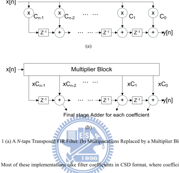
Fig. 1 (a) A N-taps Transposed FIR Filter. (b) Multiplications Replaced by a Multiplier Block . 3

Fig. 2 (a) Multiplication without CSE. (b) Multiplication with CSE ... 4

Fig. 3 BSE-based filter architecture ... 8

Fig. 4 An Example of SLSM ... 8

Fig. 5 Two Kinds of Adder Architectures ... 10

Fig. 6 An Example of Delay and Area Calculation ... 10

Fig. 7 An Example of Alphabet Selection ... 11

Fig. 8 An Example of Match Choice ... 12

Fig. 9 An Example of Sharing Issue ... 13

Fig. 10 An Example of Timing Issue ... 14

Fig. 11 GOSM Flow ... 15

Fig. 12 (a)A CAT Example. (b)The Delay and Area Calculations. ... 17

Fig. 13 Illustration for CAT(R, TrimLZ(011010)) ... 20

Fig. 14 Illustration for Sym_Enum(1010,1,1) ... 21

Fig. 15 A Pruning Example ... 24

Fig. 16 Illustrate RPCAT(C0) in Working Example ... 25

Fig. 17 The RPCAT Results for C0 and C1 ... 26

List of Tables

Table I CAT Complexity ... 22

Table II Synthesis Results of Different Adder Architectures in TSMC .18μm ... 30

Table III Results of Filters with Bitwidth of Coefficient=16 and Area & Delay Ratio=4 ... 32

Table IV Results of Filters with Bitwidth of Coefficient=12 and Area & Delay Ratio=3 ... 33

Table V Synthesis Result of Test Design: lp_32 ... 34

Table VI Results of PCAT ... 35

Table VII Results of RCAT... 36

Chapter 1

Introduction

1.1 FIR Filters in DSP System

In many digital signal processing (DSP) algorithms, finite impulse response (FIR) filter are widely used because of the advantage of stability and linear phase properties. For an

N-taps FIR filter, the input data x[n] with different time scale (0 to n-1) are multiplied by

corresponding constant coefficients Ci and then are summed up to output data y[n]. This is shown in the following equation.

y n = ∑N-1i=0 Ci·x n-1 (1.1)

Fig. 1 (a) shows an N-taps transposed FIR filter architecture which is composed of adders, multipliers and registers. In digital circuit design, multiplication is more complicated and with higher cost than add operation.

1.2 Multiple Constant Multiplications

Thus, it is important to design the multiplication operation optimally in an FIR design. Note that the architecture that multiplies the input by a set of constant coefficient is also known as multiple constant multiplications (MCM). Since the multiplier is an expansive computational unit in hardware implementation and the coefficients are mostly constants in filter design, the multiplication can be implemented by series of adders and shifters, instead of using a generalized multiplier. For example, the constant multiplication y = 5 * x can be computed as y = (x << 2) + x. The multiplier is replaced by a left shifter by 2 bits and an adder. Compared to a generalized multiplier, it reduces the hardware cost significantly. Thus, in typical digital filter designs, multiplier-less MCM is widely adopted to avoid using the costly multiplication and provide an efficient filter design. Fig. 1 (b) shows to replace

multiplications by a multiplier block and to use multiplier-less MCM to realize it.

The problem of multiplier-less MCM is similar to the classical addition chain problem where the multiplication is replaced by addition only [1]. However, the ability of using shifters and subtractors makes the multiplier-less MCM problem more complicated. The existing multiplier-less MCM algorithms can be divided into two main categories: 1) graph-based algorithms [2]-[5] and 2) digit-based algorithms [6]-[11]. The graph-based algorithms iteratively construct the graph representation in a bottom-up fashion and use heuristic methods to maximize the subexpression sharing. It can fast provide good quality of solutions (not optimal). Besides, the digit-based algorithms generate the decomposition depending on the specified binary representation.

The digit representations can be divided into two categories: 1) canonical signed-digit (CSD) 2) minimal signed-digit (MSD). CSD uses a unique signed representation (1, 0, and 1), where 1 denotes -1, for each value with two properties: 1) the number of non-zero digits (i.e., 1 _{and 1) is minimal; 2) any two consecutive non-zero digits are not adjacent (i.e.,} 1 or 1 cannot be side by side). Similar to CSD, MSD also takes the signed representation. However, it allows two adjacent non-zero digits. Thus, a variable may have more than one representation in MSD form.

Fig. 1 (a) A N-taps Transposed FIR Filter. (b) Multiplications Replaced by a Multiplier Block

Most of these implementations take filter coefficients in CSD format, where coefficients are represented with a minimum number of nonzero bits [11]. With CSD format coefficients, Common Subexpression Elimination (CSE) method has been utilized as a very powerful tool in FIR filter design to reduce the number of arithmetic units (adders and shifters). For example, consider two functions F1 and F2, where F1 = 13*x and F2 = 45*x. The CSD format

of 13 and 45 are 10101 and 1010101 so that F1 and F2 can be represented in the following

manner: F1 = 16*x - 4*x + x = x << 4 - x << 2 + x and F2 = 64*x + 16*x - 4*x + x = x << 6 +

x << 4 - x << 2 + x. The corresponding architecture is shown in Fig. 2. Both expressions F1

and F2 have some common terms or called common subexpression D = 16*x - 4*x + x.

Therefore, F1 and F2 can be rewritten as F1 = D and F2 = x << 6 + D. Reusing D in both

expressions reduces the computation overhead and the number of adders required to implement both expressions.

(a) (b) Fig. 2 (a) Multiplication without CSE. (b) Multiplication with CSE

A 2-D CSE approach, involving both vertical and horizontal eliminations, is proposed in [6]. The CSE method in [7] considers the length of critical path in the multiplier block, as well as the number of required adders. A greedy CSE algorithm with a look-ahead method for implementing low-complexity FIR filters is developed in [10]. An optimization method considering multivariable CSE is demonstrated in [8]. A level-constrained CSE (LCCSE) method is proposed in [12], it provides an analysis procedure to determine critical and less critical coefficients and constrain those critical coefficients by lower sharing.

Although, many literatures have been published, few of them discuss the problem of optimal binary subexpression sharing. We propose method that exploits patterns acquired from all possible symbols (also known as subexpressions) to match the target MCM design and model it to Integer Linear Programming (ILP) problem to optimize the delay and area. According to our experimental result, our MCM design is favorable for high speed applications.

1.3 Thesis Organization

The remainder of this thesis is organized as follows. In Chapter 2, we briefly introduce the necessary terminology and contrast against prior related works. Chapter 3 gives some motivational examples. The proposed method is demonstrated in Chapter 4. Chapter 5 shows our experimental setup and presents the experimental results. Finally, Chapter 6 gives the concluding remarks of this thesis.

Chapter 2

Background

In this chapter, we briefly review the background knowledge and the primary previous work, [14] proposes a new CSE method using binary representation of coefficients, called Binary Subexpression Elimination (BSE). Section 2.1 presents the basic terminology which we use in BSE. Section 2.2 demonstrates a heuristic method to realize the BSE architecture.

2.1 Basic Terminology

 Coefficient, C: A binary number.

 Non-zero bits, NZB(C): Number of non-zero bits in a binary number C. For example, NZB(101001)=3, NZB(11101)=4.

 Symbol, S: S is a binary number whose LSB and MSB bit are both 1’s. That is, S must be odd and without leading 0’s.

For example, 1101(S13), 11(S3), 1001(S9), 111(S7) are symbols and 110, 011, 1000 are not symbols.

 Alphabet, A: A is a set of symbols.

For example, A={1, 11, 101, 111, 1001}={S1, S3, S5, S7, S9} is an alphabet which has 5 symbols.

 Fragment, F(S, i): A number generated from left shifting the symbol S by i bits. For example, F(S5,3)=101<<3=101000.

 Match, M: A match for a coefficient C with respect to A is a set of fragments such that ∑ F_{i i}=C and ∑ NZB F_{i i} NZB C .

a match M0={F(S3,3), F(S1,1)} such that 11000+10=11010 also find M1={F(S9,1),

F(S1,3)} such that 10010+1000=11010.Identically, M2={F(S13,1)} is a match for C.

But {F(S21,0), F(S5,0)} is not a match because NZB(10101)+ NZB(101)=5, not equal to NZB(11010)=3.

2.2 Previous Works

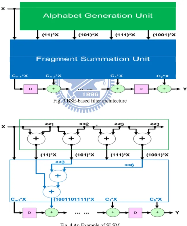
[14] proposes a new CSE method using binary representation of coefficients, called Binary Subexpression Elimination (BSE). BSE realizes a two-stage multiplier block architecture in Fig. 3. The first stage called alphabet generation unit generates binary common subexpressions or called symbols and the second stage called fragment summation unit uses these binary common subexpression to realize constant multiplication. Another application of BSE is constant multiplication for DCT which is proposed in [13].

[14] claims that their method offers average logical operator reduction of 21% over two CSE methods [15] and [16]. Even though the number of nonzero bits in the CSD representation is smaller than that in corresponding binary representation, the potential of the CSD-based CSE technique to reduce the number of adders by forming common subexpressions is less than that of binary when the number of nonzero bits is minimum.

The most important issue for BSE method is how to find out a match for a coefficient. In [14], they propose a heuristic method, called Sequential Longest Symbol Match (SLSM), which uses fixed-alphabet A={1, 11, 101, 111, 1001}. They claim that these symbols or called common subexpressions 11, 101, 111, 1001 are used to compose coefficients frequently and the reductions are not significant when other longer symbols like 10001 are used. In SLSM, we process one match at a time and sequentially match a coefficient from MSB to LSB in a piece-wise fashion. We choose the longest symbol for each partial match. Note that SLSM can only find one match for a coefficient though there are many possible solutions. For example,

assume C=1001101011. From MSB, 1(S1) or 1001(S9) can be chosen but we choose 1001(S9) instead of 1(S1) because 1001(S9) is the longest symbol where we can choose and so on. We can finally choose S9=1001 left shifts by 6 bits, S5=101 left shifts by 3 bits and S7=111. The result match is M={F(S9,6), F(S5,3), F(S3,0)} such that 1001000000+101000+11=C. After SLSM, we can use these fragment to realize the fragment summation unit, is shown in Fig. 4.

Fig. 3 BSE-based filter architecture

Chapter 3

Motivation

In this chapter, we briefly review the adder architectures and give four motivational examples to demonstrate the limitations of previous work. Based on SLSM and fixed-alphabet, we can find only one match for a coefficient. We try to find other possible matches such that we can get more benefit.

3.1 Delay and Area Calculation

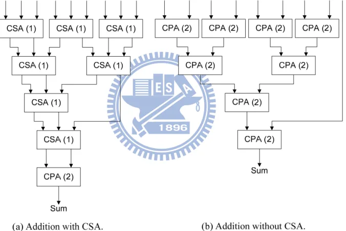
While designing a multiplier-less MCM, different adder architectures can be used depending on the design constraints. There are two kinds of widely used adder architectures, as shown in Fig. 5. General carry propagation adder (CPA) adds two numbers x and y to a number a. The carry save adder (CSA) takes three numbers, x, y, and z, and transform it to two numbers, a and b, such that x + y + z = a + b. Note that the output of CSA are not the final summation result. An extra CPA is required to calculate the final two subexpressions, CSA is preferred to iteratively cover the subexpressions then use a CPA to get the final results.

Because CPA is more complicated than CSA, we assume the delay and area ratio of CPA and CSA is 2. For a 9 number adder operation, we use 7 CSA with 1 CPA to realize this operation in Fig. 6 (a) rather than 8 CPA operations in Fig. 6 (b), so that we can reduce 7 units area and 2 units delay.

Fig. 5 Two Kinds of Adder Architectures

Fig. 6 An Example of Delay and Area Calculation

3.2 An Example of Alphabet Selection

In SLSM process, the number of fragments in result match rests with the length of symbols where we choose in each partial selection from fixed-alphabet. Thus, in this example,

we add a longer symbol 10001 in Alphabet which is called A1 and try to reduce the number of fragments in result match.

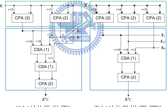
We use SLSM with the coefficient C=1111000110010 to realize the alphabet generation unit and the fragment summation unit. Fig. 7 (a) shows the circuitry that corresponds to the match Ma={F(S7,10), F(S1,9), F(S3,4) , F(S1,1)} with alphabet A0={1, 11, 101, 111, 1001} and Fig. 7 (b) shows the circuitry that corresponds to an alternative match Mb={F(S7,10),

F(S17,5), F(S9,1)} with alphabet A1. Obviously, the fragment summation unit reduces 1 CSA

cost that is equal to save 1 unit area and 1 unit delay. By adding longer symbol, it takes different alphabet and probably can get more efficient fragment summation unit.

Fig. 7 An Example of Alphabet Selection

3.3 An Example of Match Choice

of 1’s in the coefficient should be corresponded to a fragment. The following example shows an alternative match where we use an interleaving way such to cover all of 1’s in the coefficient.

We use a fixed-alphabet A=A0 and assume coefficient C=1001101101. Fig. 8 (a) shows the result Ma={F(S9,6), F(S5,3), F(S5,0)} based on SLSM. But the pattern 101101 in C can separate to two fragment F(S9,2) and F(S9,0) instead of F(S5,3) and F(S5,0) by an interleaving way. An alternative match Mb={F(S9,6), F(S9,2), F(S9,0)} is shown in (b). In this case, we can eliminate the symbol S5 which is not used by getting different match so that the alphabet generation unit can reduce 2 units area.

Fig. 8 An Example of Match Choice

3.4 An Example of Sharing Issue

In major MCM methods, common subexpression sharing is an important way to reduce the hardware cost. But SLSM does not consider other coefficients when process a coefficient.

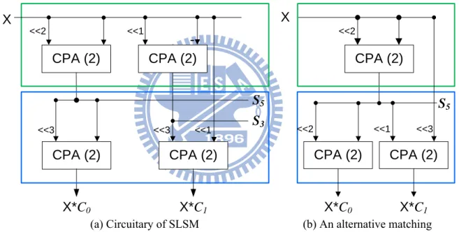
To consider more coefficients, the two coefficient C0=101101 and C1=011010 are used as this example.

Fig. 9 (a) shows SLSM result Ma0={F(S5,3), F(S5,0)} for C0 and Ma1={F(S3,3), F(S1,1)} for C1 . However, we can find another efficient matches Mb0={F(S5,3), F(S5,3)} for C0 and

Mb1={F(S5,1), F(S1,3)} for C1 as shown in (b). Take Ma1 and Mb1into comparison, Mb1 uses

the same symbol S5 in Mb0 without generating a new symbol S3. On alphabet generation unit, we can save 2 units area. In this case, we try to use a common symbol S5 to realize the two coefficients instead of process the two coefficients individually.

<<2 CPA (2) <<1 X*C0 CPA (2) CPA (2) X S5 S3 CPA (2) X <<2 CPA (2) X*C0 S5

(a) Circuitary of SLSM (b) An alternative matching

CPA (2) X*C1 CPA (2) X*C1 <<2 <<1 <<3 <<3 <<3 <<1

Fig. 9 An Example of Sharing Issue

3.5 An Example of Timing Issue

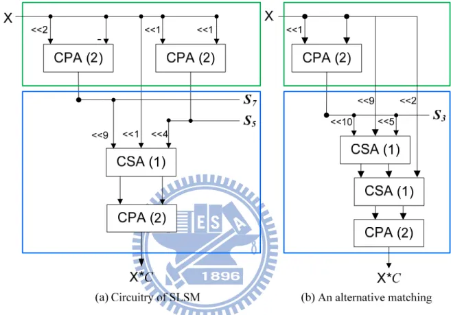
SLSM cannot take a trade-off between area and delay because of its fixed result. Under different timing constraint, we must choose a suitable match for a coefficient rather than a changeless match.

The following example shows two different matches, we assume coefficient C=111000110010 and alphabet is A0. Fig. 10 (a) shows that the match Ma={F(S7,9), F(S3,4),

F(S1,1)} is found by SLSM and (b) shows another match Mb={F(S3,10), F(S1,9) , F(S3,4), F(S1,1)}. Compared to Ma, maximum delay of Mb is longer than Ma but Mb has small area cost

than Ma. In our work, we provide users for a timing constraint, extend all of possible matches under this timing constraint and decide a best solution.

Fig. 10 An Example of Timing Issue

3.6 Problem Formulation

In this thesis, we address the problem of optimal MCM design based on two stage multiplier block architecture. We are given:

 a set of fixed-point coefficient {C0, C1…, Cn-1},

 the timing constraint from input X to output of fragment summation unit X*C,  the delay and area ratio of CSA and CPA.

Our goal is to minimize total area cost including alphabet generation unit and fragment summation unit under the given timing constraint.

Chapter 4

Our Proposed Algorithm

In this chapter, we describe our algorithm, called Global Optimal Symbol Match (GOSM), which can find out matches for coefficients and implement the delay and area optimal BSE-based FIR filters. Section 4.1 presents our algorithm including terminology (4.1.1), pseudo code (4.1.2), complexity analysis (4.1.3) and two enhanced methods (4.1.4 and 4.1.5). Section 4.2 illustrates a working example. Finally, section 4.3 gives Integer Linear Programming (ILP) formulation to optimize delay and area.

4.1 Algorithm Flow

The detail processes are shown in Fig. 11. Step 1, we enumerate all possible matches and construct the Coefficient Assembly Tree (CAT). Step 2, to reduce the complexity, we eliminate the redundant paths. Step 3, we use ILP to decide the best paths for all coefficients.

4.1.1 Terminology

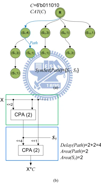
 Coefficient Assembly Tree, CAT(C): A tree which is extended for a coefficient C. For example, Fig. 12 (a) illustrates a CAT for a coefficient C=6’b011010.

 Path: A match which is from root to leaf in CAT(C).

For example, in Fig. 12 (a), The CAT includes 5 paths which correspond to 5 possible matches for this coefficient.

 SymSet(Path): A set of symbol that are used on Path.

For example, the marked path in Fig. 12 (a) includes two fragment, (S1,4) and (S5,1), therefore, SymSet(Path)={S1,S5}.

 Delay(Path): Delay of Path including symbol generation time.

For example, Fig. 12 (b) shows the implementation of alphabet generation unit and fragment summation unit which correspond to the Path={(S1,4),(S5,1)}. The maximum delay is 4 which is from X to X*C.

 Area(Path): Area cost of Path.

For example, we use a CPA to add two fragment, (S1,4) and (S5,1), is shown in below frame of Fig. 12 (b).

 Area(S): Area cost of symbol S.

For example, we use two symbols, S1 and S5, on this Path, since the alphabet generation unit includes two area cost, Area(S1)=0 and Area(S5)=2.

 Trim leading zero’s, TrimLZ(C): Trim the leading 0’s in C. For example, TrimLZ(011010)=11010 , TrimLZ(0001011)=1011.  Trim MSB, TrimMSB(C): Trim the MSB in C.

For example, TrimMSB(11010)=1010.

 |C|: Bitwidth of TrimLZ(C), where C is a binary number. For example, |1001|=4, |011010|=5, |11010|=5.

 Difference of length, DOL(C, S): Return |C|-|S|, where C is a coefficient and S is a symbol.

For example, DOL(11010,1001)=5-4=1 , DOL(11010,11)=5-2=3.  Residue(B, C): TrimLZ(B-C), where B and C are binary numbers.

For example, Residue(11010,10010)=TrimLZ(11010-10010)=TrimLZ(01000)=1000.

(a)

(b)

4.1.2 Coefficient Assembly Tree Enumerator

CAT enumerator enumerates a CAT for a coefficient. To find out all CATs, we execute CAT enumerator n times for n coefficients in coefficient set. The recursive pseudo code for CAT enumerator as follows.

Initial: A=;

CAT (Root, TrimLZ(C))

1 Symbol=;

2 for num_1 from 0 to NZB(C)-1 3 C’=TrimMSB(C);

4 S=1;

5 Sym_Enum(C’, S, num_1); 6 foreach S  Symbol

7 d=DOL(C, S);

8 create a child node r=F(S, d) for Root; 9 add symbol S into alphabet A;

10 CAT(r, Residue(C, S<<d)); End Sym_Enum(C’, S, num_1) 1. if(num_1==0) 2. add S to Symbol; 3. return; 4. if(MSB(C’)==0)

5. Sym_Enum(TrimMSB(C’), S<<1, num_1);// skip current 0 6. else// MSB(C’) == 1

7. if(NZB(C’)>num_1) // enough remaining 1’s? 8. Sym_Enum(TrimMSB(C’), S<<1, num_1);// skip current 1 9. Sym_Enum(TrimMSB(C’), S<<1+1, num_1-1);// pick current 1 End

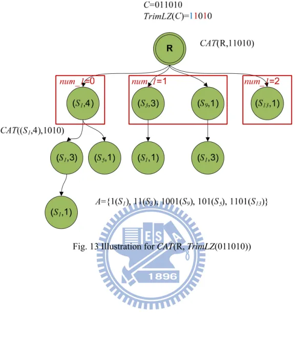
Note that, the alphabet A is empty initially. To simplify the calculation we trim the leading zero’s in C, before starting CAT. The first for loop in line 2 to line 5 generates the useable symbol. Num_1 indicates the number of 1’s which must be chosen in C’. For example,

assume C=011010 C’=TrimMSB(11010)=1010, it means zero 1‘s-combinations from two 1’s in C’(C ), one 1’s-combinations from two 1’s in C’(C ) and two 1’s-combinations from two 1’s in C’(C ), after the for loop, by three kinds of different combinations we can get 4 possible symbols 1(S1), 11(S3), 1001(S9), 1101(S13) and add them to a set Symbol. The second for loop in line 6 to line 10, for each symbol S in Symbol, we create a child node r= F(S, d) where d is

DOL(C, S), add S into A and use the Residue(C, S<<d) to recursive call CAT. For example, we

create a child node r=F(1,d) for Root where d is DOL(011010,1)=4, add 1(S1) to A and call

CAT(r,1010). The recursive call terminates when the first for loop don’t generate any

symbols.

The Sym_Enum is a sub-function in CAT line 5 which is used to generate the useable symbol for C. Before starting Sym_Enum, we trim the first 1 in C to an initial symbol S. By

Sym_Enum, the symbol S grows up to those useable symbols and stores in the set Symbol. In

each recursive call, we check the MSB(C’). If it’s 0, we skip this bit, let S<<1 and recursive call Sym_Enum for TrimMSB(C’). If it’s 1, we can skip this 1 as a 0 if the remaining 1’s in C’ still enough also we can pick this 1 and let (S<<1)+1 and decrease the index num_1 by 1. The recursive call terminates when num_1 counts down to 0. An example for

Sym_Enum(1010,1,1) is illustrated in Fig. 14. In this example, S grew up to 11(S3) and

Fig. 14 Illustration for Sym_Enum(1010,1,1)

4.1.3 Coefficient Assembly Tree Complexity

The analysis of CAT complexity, we try to find out NumP(k).

 NumP(k): Number of possible path in CAT(C) such that NZB(C)=k.

Actually, NumP(k) is only related to NZB(C). For example, the CAT of 10011 and the CAT of 11001 have identical number of paths because of their identical number of non-zero bits. According to CAT enumerator, the recursive equation as follows

  1, k 0, 1       

∑ C ∙ i 1 , otherwise (4.1)

, where C_ik-1 represents i-combination from n-1 bits.

NumP(3)= C₀2·NumP(2)+ C₁2·NumP(1)+ C₂2·NumP(0) =1*2+2+1=5. Table I shows NumP(k)

from k=0 to k=12.

Table I CAT Complexity

NZB(C) NumP(k) NZB(C) NumP(k) NZB(C) NumP(k)

0 1 5 52 10 115975

1 1 6 203 11 673224

2 2 7 877 12 4213597

3 5 8 4140 >12 >4213597

4 15 9 21147

4.1.4 Pruned Coefficient Assembly Tree

To consider the timing issue, during enumerating CAT, we can check maximum delay and prune those paths which are over timing constraint. The pseudo code of the modified

CAT, called PCAT is as follows.

Initial: A=;

Pathmiddle=;

PCAT (Root, TrimLZ(C), Pathmiddle)

1 Symbol=;

2 for num_1 from 0 to NZB(C)-1 3 C’=TrimMSB(C);

4 S=1;

5 Sym_Enum(C’, S, num_1); 6 foreach S  Symbol

7 d=DOL(C, S);

8 add F(S, d) to Pathmiddle;

9 if(Delay(Pathmiddle)<timing constraint)

12 PCAT(r, Residue(C, S<<d), Pathmiddle);

End

The differences between CAT and PCAT are marked by bold text. To calculate maximum delay of Path, we call PCAT with Pathmiddle and record every node we enumerate. The significant difference is that, before creating a childe node, we must estimate the delay if the child node F(S, d) add to a temporary path Pathmiddle, corresponding to line 8 and line 9.

For example, the coefficient C is 11011101 and we assume the delay and area ratio of CPA and CSA is 2 and the timing constraint is 5. When we execute to the node F(S5, 4) in Fig. 15, PCAT(F(S5,4), 1101, {F(S1,7), F(S5,4)}), we add the node F(S1,3) with an arrow to

Pathmiddle and calculate the maximum delay of Pathmiddle={F(S1,7), F(S5,4), F(S1,3)} to decide

whether we create child node F(S1,3) or not. Because the delay of Pathmiddle is 5, which is equal to the timing constraint, PCAT for node F(S1,3) will not be execute. By pruning on

F(S1,3), Those child nodes of F(S1,3) which are marked by dash circle will not be enumerated.

Pruned Coefficient Assembly Tree (PCAT) may not be enumerated completely as CAT since the complexity will not be as pessimistic as our analysis in section 4.1.3. In the following chapter (5.4), we will show the reduction rate by pruning with different timing constraint.

Fig. 15 A Pruning Example

4.1.5 Reduced Pruned Coefficient Assembly Tree

In this section, we propose a method, called reduction phase to reduce Coefficient Assembly Tree complexity again. Once a path is completed in PCAT process (not create any child node), we check SymSet(Path) and Area(Path) to decide whether we eliminate this path or not. Similar to SymSet(Path), we store the smallest area path from those path have completed so far. Since we only reserve the smallest area path for a kind of SymSet(Path). Using hashtable technique, we can realize SymSet(Path) check in linear time. For example, if the area ratio of CPA and CSA is 2 and coefficient C=11011101, we assume a path1 ={F(S1,7),F(S5,4),F(S1,3),F(S1,2),F(S1,0)} with respect to SymSet(Path1)={S1, S5} store in the temporary in previous action then a path2={F(S1,7),F(S5,4),F(S1,3),F(S5,0)} with respect to SymSet(Path2)={S1, S5} now is completed. Because they have same SymSet and

Area(Path2)=4 is smaller than Area(Path1)=5, we replace path1 by path2 into the temporary. path1 is a redundant path in this case, eliminate path1 does not affect our optimal solution

because Path2 is a better choice whatever considering other coefficient. In chapter 5, we show that the reduction phase can reduce about 20% total number of paths.

4.2 Working Example

We illustrate a complete example with two coefficients. The coefficient set is {101101(C0), 011010(C1)} and the delay and area ratio of CPA and CSA is 2, the timing constraint is 4. Fig. 16 shows the overall process, and deep color node indicates a pruning occur because of its timing violation. After executing PCAT for C0, an alphabet A extends completely. For each coefficient, through PCAT enumerator and reduction phase, we can get two RPCAT and there are five paths for each coefficient, as shows in Fig. 17.

Fig. 17 The RPCAT Results for C0 and C1

4.3 Integer Linear Programming (ILP) Formulation

In the previous section, we enumerate all possible matches and construct the CAT. Secondly, we form our problem to an ILP problem and use ILP solver to decide the best paths for all coefficients.

4.3.1 Variables

In the proposed ILP formulation, two variables are used to model the behavior of choosing a path in a CAT. First, VarPath indicates whether the path is selected or not. The other one is VarS which means the symbol selection in the alphabet. The following equation

lists the corresponding ILP formulations.

VarPath_i,j 1, if Pathi,j is chosen by ILP solver.      

0, if Path_i,j is not chosen by ILP solver. (4.2)

VarS_{i 0, if S}1, if Si is chosen by ILP solver.

i is not chosen by ILP solver.

(4.3)

4.3.2 Objective Function

Our proposed FIR filter is a two stage architecture, alphabet generation unit and fragment summation unit. Since VarS is a 0-1 variable, we can calculate the area of alphabet generation unit by ∑ Area(Si)·VarSi . Similarly, VarPath is also a 0-1 variable. The area of fragment summation unit can be calculated by similar equation, such as ∑ ∑ Area(Pathi,j)·VarPathi,j . In order to minimize the total area cost, the objective

function can be formulated as:

∑ Area(Si)·VarSi ∑ ∑ Area(Pathi,j)·VarPathi,j (4.4)

where n is number of coefficients

k is number of paths in ith coefficient and m is number of symbols in alphabet A.

4.3.3 Existence Constraint

In CAT, each path means a kind of implementation, which is composed by many symbols. If a Pathi,j is selected the corresponding symbols should be also existed in the alphabet, i.e. S  SymSet(Pathi,j).Therefore, the existence constraint is used to guarantee all of the symbols of the selected path is existed in the alphabet. The formulation is as follows:

VarPathi,j≤ min{VarS0,…, VarSn-1} ∀ Path_i,j|S SymSet(Pathi,j) (4.5)

A coefficient can be produced by several implementations. If multiple implementations are chosen, it results in hardware waste. In order to ensure only one path is chosen for a coefficient, the uniqueness constraint should be accordingly formulated as:

∑ VarSi

k-1

j=0 1  (4.6)

where k is number of paths for the coefficient

4.3.5 ILP Example

In section 4.2, we illustrate the example with two coefficients. After above procedure, we can get 5 possible paths for each coefficient C0 and C1 as show in Fig. 17. Then, the objective

is minimized

4VarPath0,0+2VarPath0,1+2VarPath0,2+2VarPath0,3+0VarPath0,4+ 3VarPath1,0+2VarPath1,1+2VarPath1,2+2VarPath1,3+0VarPath1,4+

0VarS1+2VarS3+2VarS5+2VarS9+3VarS11+3VarS13+3VarS37 +3VarS41+4VarS45. In addition, the corresponding constraints are listed below:

Existence constraint:

VarPath0,0≤ min{VarS1}; VarPath0,1≤ min{VarS5};

VarPath0,2≤ min{VarS9}; VarPath0,1≤ min{ VarS3, VarS33}; VarPath0,4≤ min{VarS45};

VarPath0,0≤ min{VarS1}; VarPath0,1≤ min{VarS5}; VarPath0,2≤ min{VarS3}; VarPath0,1≤ min{VarS9};

Uniqueness constraint:

VarPath0,0+VarPath0,1+VarPath0,2+VarPath0,3+VarPath0,4=1; VarPath1,0+VarPath1,1+VarPath1,2+VarPath1,3+VarPath1,4=1.

Eventually, we use ILP solver, named gurobi [17] to solve this ILP problem. The ILP result is VarPath0,2=1, VarPath1,3=1 and VarS9=1, as shown in Fig. 18 and the best solution is

Area(Path0,2)+Area(Path1,3)+Area(S9)=2+2+2=6.

Chapter 5

Experimental Results

5.1

Experiments

Setup

The proposed BSE algorithm, GOSM, is developed in C++/Linux environment. We also use this environment to develop SLSM [14]. The coefficient sets of these test designs are generated by Matlab FDAtool [18].

Two widely used CPA architectures. First, a ripple carry adder (RCA) is the simplest adder structure where the carry bit must wait for the previous full adder. Thus, the critical path delay is relatively longer than other adder structures. Second, a carry look-ahead adder (CLA) calculates the carry bits before the sum, which reduce the critical path delay dramatically.

Table II reports the synthesis results of these two CPA and CSA (refer to 3.1) architectures with different bitwidth under TSMC 180nm process. It apparently shows that RCA is the smallest with longer computation time and CSA is fastest with linear area increasing. Thus, in high speed application, such as software defined radio (SDR), it is desired to design a filter with shorter critical path delay. Therefore, we choose CLA as CPA and decide that area ratio is 4(1368/376) in 16 bitwidth, 3(968/306) in 12 bitwidth and delay ratio is 4(1.2/0.32) in 16 bitwidth, 3(0.95/0.32) in 12 bitwidth.

Table II Synthesis Results of Different Adder Architectures in TSMC .18μm

Architectures 4-bit 8-bit 12-bit 16-bit

RCA Delay(ns) 2.05 2.85 3.92 4.99 Area (μm2) 134 141 211 282 CLA Delay(ns) 0.60 0.79 0.95 1.2 Area (μm2) 301 814 968 1368 CSA Delay(ns) 0.32 0.32 0.32 0.32 Area (μm2) 190 235 306 376

5.2 Case Study I : Versus SLSM

Table III/IV illustrates 10 filter designs with 16/12 bitwidth coefficients, named lp (lowpass), hp (highpass), bp (bandpass), bs (bandsotp) and their filter length. The area & delay ratio is 4/3 for 16/12 bitwidth. First, we find out maximum delay and area cost for all designs by using SLSM method as show in 2nd and 3rd columns. Then, we use those Maximum delays as our timing constraints in GOSM method and the corresponding area result are shown in right side columns. Rate is the percentage of (area cost by SLSM-area cost by GOSM)/area cost by SLSM and #sym. represents number of symbols which ILP solver actually chooses in GOSM.

Under same timing constraint, GOSM can minimize area cost average 26/22% in 16/12 bitwidth with timing constraint. Using SLSM, with the growth of the filter length, the area cost of filter increase linearly. But in GOSM, the area cost of filter increase slower. Furthermore, by using GOSM, ILP solver chooses not only five symbols (avg. 18.) but grew up with the filter length. For longer length filters, the complex symbols appear in coefficient frequently. The benefit of those complex symbols causes the different of the reduction ratio between SLSM and GOSM in longer length filters. Therefore, the reduce ratio of area cost and the length of filter are in direct proportion.

GOSM can find the solutions when timing constraint is tighter which illustrate in rows of delay-2 and delay-1 since it expand the solution space. The Reduction rate of maximum delay is at most 20%.

Table III Results of Filters with Bitwidth of Coefficient=16 and Area & Delay Ratio=4

Designs SLSM GOSM

filter delay area delay delay-1 delay-2

area (rate) #sym. area (rate) #sym. area (rate) #sym.

bs_31 10 92 77 (16.3%) 6 80 (13%) 7 97 (-5.4%) 10 lp_32 10 89 76 (14.6%) 6 80 (10.1%) 8 95 (-6.7%) 9 hp_63 10 144 126 (12.5%) 10 138 (4.2%) 8 166 (-15.3%) 12 bp_64 11 156 135 (13.5%) 11 135 (13.5%) 12 147 (5.7%) 11 lp_127 10 231 186 (19.5%) 13 189 (18.2%) 13 234 (-1.3%) 22 bp_128 10 306 248 (18.9%) 17 271 (11.4%) 17 344 (-12.4%) 33 hp_255 10 387 267 (31%) 27 276 (28.7%) 27 311 (19.6%) 33 lp_256 10 395 254 (35.7%) 21 262 (33.7%) 21 300 (24.1%) 26 bs_511 10 626 354 (43.5%) 35 357 (43%) 35 424 (32.3%) 44 lp_512 10 820 378 (53.9%) 36 387 (52.8%) 36 440 (46.4%) 44 Avg. 10.1 324.6 210.1 (26%) 18.2 217.5 (23%) 18.4 255.8 (16.3%) 24.4

Table IV Results of Filters with Bitwidth of Coefficient=12 and Area & Delay Ratio=3

Designs SLSM GOSM

filter delay area delay delay-1 delay-2

area (rate) #sym. area (rate) #sym. area (rate) #sym.

bs_31 7 45 38 (15.6%) 6 43 (4.4%) 7 lp_32 7 38 33 (13.2%) 5 38 (0%) 5 hp_63 7 61 53 (13.1%) 8 62 (-1.6%) 8 bp_64 8 67 57 (15%) 9 57 (15%) 10 66 (1.5%) 10 lp_127 7 76 54 (28.9%) 9 57 (-25%) 10 bp_128 7 124 109 (12.1%) 13 hp_255 7 93 64 (31.2%) 12 70 (24.7%) 13 lp_256 7 80 56 (30%) 12 59 (26.3%) 12 bs_511 7 106 72 (32.1%) 12 lp_512 7 125 86 (31.2%) 14 93 (25.6%) 14 Avg. 7.1 81.5 62.2 (22.2%) 10 59.9 (8.7%) 9.9 66 (1.5%) 10

5.3 Case Study II : Synthesis Result

We use synopsys Design Compiler [19] and TSMC 0.18μm CMOS process on a workstation. Table V illustrates the synthesis result of test design: lp_32 with 16 bitwidth coefficients.

Compared GOSM with SLSM, our estimations are given from Case Study I multiplied by 1 CSA unit factor and corresponding synthesis results are shown in right side. In this design, we a little over estimate about 13% in delay and 6.6% in area. In Diff. row, we estimate GOSM can reduce 20% delay but increase 6.74% area overhead. Actually, GOSM can reduce 21% delay but increase 7.1% area overhead. It is means that the reduction rate in

Table III and IV can accurately correspond to their synthesis result.

Table V Synthesis Result of Test Design: lp_32

Algorithms

Our estimation Synthesis Result of Multiplier

Block (error rate)

Delay(ns) Area(μm2) Delay(ns) Area(μm2)

SLSM 10*0.32=3.2 89*376=33464 2.8 (12.5%) 31201.6 (6.7%)

GOSM 8*0.32=2.56 95*376=35720 2.2 (14.4%) 33420.3 (6.5%)

Diff. 20% -6.74% 21% -7.1%

5.4 Case Study III : Pruned CAT

In this case study, Table VI shows the comparison of number of paths without/with pruning (section 4.1.4). The bitwidth of coefficient is 16. 2nd column shows number of paths without pruning, CAT algorithm. Right side columns show number of paths using PCAT algorithm with 8~11 timing constraints. Number of paths extremely decreases to less than 5% remaining with 8 timing constraint. Under 10 timing constraint, pruning technique also reduces average 37.5% number of paths.

Table VI Results of PCAT

Designs # of possible paths with reduction phase(reduction rate)

filter Without pruning Timing constraint 11 10 9 8 bs_31 5447 5196 (4.6%) 3411 (37.4%) 494 (91%) 49 (99.1%) lp_32 1842 1821 (1.1%) 1590 (13.7%) 435 (76.4%) 49 (97.3%) hp_63 27200 24893 (8.5%) 8464 (68.9%) 635 (97.7%) 113 (99.6%) bp_64 21003 19909 (5.2%) 12359 (41.2%) 846 (96%) 120 (99.4%) lp_127 9413 9094 (3.4%) 6714 (28.7%) 1272 (86.5%) 216 (97.7%) bp_128 58780 53944 (8.2%) 19479 (66.9%) 1711 (97.1%) 236 (99.6%) hp_255 18684 17834 (4.5%) 11869 (36.5%) 1830 (90.2%) 463 (97.5%) lp_256 18077 17213 (4.8%) 11268 (37.7%) 1618 (91%) 487 (97.3%) bs_511 16912 16452 (2.7%) 12944 (23.5%) 2757 (83.7%) 829 (95.1%) lp_512 16521 16139 (2.3%) 13082 (20.8%) 4284 (74.1%) 1068 (93.5%) Avg. 19387.9 18249 (4.5%) 10118 (37.5%) 1588 (88.4%) 363 (97.6%)

5.5 Case Study IV : Reduced CAT

Table VII shows the comparison of number of paths before/after reduction phase (section 4.1.5). The bitwidth of coefficient is 16.There is no timing constraint and pruning occurrence. In # of possible paths column, reduction phase can reduce average 27.8% number of paths and save the run time of ILP solver. In bp_128 this case, we can extra cost no more than 1 sec on enumerating RCAT but get about 50% speedup on ILP solving time. By using reduction phase, we can reduce ILP solver overhead, only increase a little enumerating time.

Table VII Results of RCAT

Designs Before reduction After reduction

filter # of possible paths Run time(sec.) # of possible paths (reduction rate)

Run time(sec.)

Tree ILP Tree ILP

bs_31 5447 0.8 1.09 3965 (27.2%) 1.43 0.61 lp_32 1842 0.22 0.15 1428 (22.5%) 0.84 0.12 hp_63 27200 12.6 17.74 19782 (27.3%) 13.53 8.85 bp_64 21003 6.74 5.16 13789 (34.3%) 7.78 2.34 lp_127 9413 1.95 0.62 6786 (27.9%) 4.39 0.36 bp_128 58780 40.19 73.34 43710 (25.6%) 40.89 37.67 hp_255 18684 4.6 1.82 12930 (30.8%) 9.46 0.92 lp_256 18077 5.06 2.26 12732 (29.6%) 9.96 0.97 bs_511 16912 3.87 1 12179 (28%) 13.37 0.59 lp_512 16521 3.61 0.93 12393 (25%) 13.5 0.65 Avg. 19387.9 7.96 10.41 13969.4 (27.8%) 11.29 5.31

5.6 Case Study V : Reduced Pruned CAT

Combining pruning with reduction phase, Table VIII illustrate the results of RPCAT. Table VIII is the result of Table VI with reduction phase. Compared to Table VI, RPCAT also has the same tendency on timing axis but overall reduce about 20% number of path when timing constraint is 9~11. We succeed in reducing CAT complexity by using above two strategies.

Table VIII Results of RPCAT

Designs # of possible paths with reduction phase(reduction rate)

filter Without pruning Timing constraint 11 10 9 8 bs_31 3965 3725 (6.1%) 2397 (39.5%) 397 (90%) 49 (98.8%) lp_32 1428 1407 (1.5%) 1186 (17%) 336 (76.5%) 49 (96.6%) hp_63 19782 17636 (10.8%) 5940 (70%) 450 (97.7%) 111 (99.4%) bp_64 13789 12800 (7.2%) 7591 (44.9%) 575 (95.8%) 113 (99.2%) lp_127 6786 6481 (4.5%) 4641 (31.6%) 1017 (85%) 214 (96.8%) bp_128 43710 39167 (10.4%) 14120 (67.7%) 1260 (97.1%) 226 (99.5%) hp_255 12930 12121 (6.3%) 7673 (40.7%) 1409 (89.1%) 447 (96.5%) lp_256 12732 11902 (6.5%) 7471 (41.3%) 1255 (90%) 469 (96.3%) bs_511 12179 11737 (3.6%) 8793 (27.8%) 2118 (82.6%) 786 (93.5%) lp_512 12393 12019 (3.1%) 9403 (24.1%) 3223 (74%) 1000 (92%) Avg. 13969.4 12899 (6%) 6921.5 (40.5%) 1204 (88%) 346 (96.9%)

Chapter 6

Conclusions & Future Works

In this thesis, Global Optimal Symbol Match (GOSM) is proposed for FIR filer synthesis. This method explores a large solution space, gives an optimal solution under the given timing constraint by formed ILP problem, provides a delay and area optimal BSE-based FIR filters and makes trade-off between area and delay.

Compared to SLSM, under the same timing constraint, GOSM reduces area cost about 25% and reduces maximum delay at most 20%.

According to case study II, BSE-based FIR filter by GOSM method can achieve up to about 400MHz clock rate in .18μm process and it could be suitable for high speed DSP applications.

We also propose two different kinds of method, PCAT and RCAT to reduce the complexity of coefficient assembly tree. PCAT reduces 37.5% number of paths when the timing constraint is 10. RCAT takes at most 50% speedup on ILP solving time.

GOSM produces an optimal solution in BSE architecture with two reduction methods to seamless minimize the complexity of coefficient assembly tree. However, for some coefficient, the number of paths is still large and takes too much long time for ILP solver. From those cases which NZB(C) is much bigger (i.e., up to 13 bits), we can separate this coefficient C to some sub-coefficients and then their non-zero bits would be smaller. Although the optimal property is scarified, a good-quality BSE-based filter can be still generated for an extremely large filter case.

References

[1] K. Parhi, VLSI Digital Signal Processing Systems: Design and Implementation. New York: Wiley, 1999.

[2] D. R. Bull and D. H. Horrcks, “Primitive operator digital filters,” Proceeding Inst. Elect.

Eng.—Circuits Devices Systems, vol. 138, no. 3, pp. 401–412, Jun. 1991.

[3] A. G. Dempster and M. D. Macleod, “Use of minimum-adder multiplier blocks in FIR digital filters,” IEEE Transactions on Circuits and Systems. II, Analog Digital Signal

Process, vol. 42, no. 9, pp. 569–577, Sep. 1995.

[4] H.-J. Kang and I.-C. Park, “FIR filter synthesis algorithms for minimizing the delay and the number of adders,” IEEE Transactions on Circuits and Systems. II, Analog Digital

Signal Process, vol. 48, no. 8, pp. 770–777, Aug. 2001.

[5] A. Dempster et al., “Designing multiplier blocks with low logic depth,” IEEE

international symposium on Circuits and Systems, May 2002, vol. 5, pp. 773–776.

[6] Y. Takahashi and M. Yokoyama, “New cost-effective VLSI implementation of multiplierless FIR filter using common subexpression elimination," IEEE international

symposium on Circuits and Systems, May 2005, vol. 2, pp. 1445–1448.

[7] C. Yao, H. Chen, T. Lin, C. Chien and C. Hsu, “A novel common subexpression elimination method for synthesizing fixed-point FIR filters,” IEEE Transactions on

Circuits and Systems I, pp. 2211–2215, Nov. 2004.

[8] A. Hosangadi et al., “Algebraic methods for optimizing constant multiplications in linear systems,” J. VLSI Signal Process Systems, vol. 49, no. 1, pp. 31–50, Oct. 2007.

[9] O. Gustafsson and L. Wanhammar, “ILP modelling of the common subexpression sharing problem,” IEEE International Conference on Electronics, Circuits and Systems, Dec. 2002, vol. 3, pp. 1171–1174.

implementing FIR filters,” IEEE international symposium on Circuits and Systems, May 2007, pp. 3451–3454.

[11] R. M. Hewlitt and E. S. Swartzlander, “Canonical signed digit representation for FIR digital filters,” IEEE Workshop on Signal Processing Systems, 2000, pp. 416–426.

[12] J. H. Choi, et al., "Variation-aware low-power synthesis methodology for fixed-point FIR filters," IEEE Transactions on Computer-Aided Design Integrated Circuits and Systems, vol. 28, pp. 87-97, 2009.

[13] G Karakonstantis, N. Banerjee and K. Roy, “Process-variation resilient and voltage-scalable DCT architecture for robust low-power computing,” IEEE Transactions

on Very Large Scale Integrated Systems, pp. 1461-1470, 2010.

[14] R. Mahesh and A. P. Vinod, “A new common subexpression elimination algorithm for realizing low complexity higher order digital filters,” IEEE Transactions on

Computer-Aided Design Integrated Circuits and Systems, pp. 217–219, Feb. 2008.

[15] M. M. Peiro, E. I. Boemo, and L. Wanhammar, “Design of high-speed multiplierless filters using a nonrecursive signed common subexpression algorithm,” IEEE

Transactions on Circuits and Systems. II, Analog Digital Signal Process, vol. 9, no. 3, pp.

196–203, Mar. 2002.

[16] F. Xu, C. H. Chang, and C. C. Jong, “Contention resolution algorithm for common subexpression elimination in digital filter design,” IEEE Trans. Circuits Syst. II, Exp.

Briefs, vol. 52, no. 10, pp. 695–700, Oct. 2005.

[17] Gurobi optimizer online[available] http://www.gurobi.com/ [18] Matlab FDAtool