混合的偏斜常態分布其及應用

全文

(1)國立交通大學統計學研究所碩士論文混合的偏斜常態分佈及其應用 On the mixture of skew normal distributions and its applications. 研究生：顏淑儀指導教授：李昭勝博士林宗儀博士. 中華民國九十四年六月.

(2) 混合的偏斜常態分佈及其應用 On the mixture of skew normal distributions and its applications 研究生：顏淑儀指導教授：李昭勝林宗儀. Student：Shu-Yi Yen Advisor：Dr. Jack C. Lee Dr. Tsung I. Lin. 國立交通大學統計學研究所碩士論文 A Thesis Submitted to Institute of Statistics College of Science National Chiao Tung University in Partial Fulfillment of the Requirements for the Degree of Master in Statistics June 2005. Hsinchu, Taiwan, Republic of China 中華民國九十四年六月.

(3) 混合偏斜的常態分佈及其應用研究生：顏淑儀. 指導教授：李昭勝博士林宗儀博士. 國立交通大學統計學研究所. 摘要混合的常態分佈對於來自不同來自母體的異質性資料提供了一種的自然模型架構。近二十年來，偏斜的常態分佈對於處理非對稱的資料問題已被驗證是一種很有用的工具。本文我們提出了以概似函數與貝氏抽樣為基礎之方法去處理混合偏斜常態分佈的問題。我們將利用＂期望最大值型式＂(EM-type)演算法求最大概似估計值。對於所提出的先驗分佈及所推導之後驗分佈的結果, 我們也運用馬可夫鏈蒙地卡羅發展出貝氏的計算方法。最後我們透過兩個實例來闡述所提出模型之應用。.

(4) 致謝研究所兩年的生涯，在快樂、充實、努力的時刻中，匆匆的過去了，在面臨口試通過即將要畢業的時刻，中心百感交集，期待與不捨的情緒錯綜複雜，當然此刻心情充滿了感激及感動。論文得以順利的完成，首先要感謝的就是我的指導教授李昭勝老師，老師豐富的學識涵養和對於學生的關心和照顧，都讓我受益良多、心存感激，身為李老師的學生讓我覺得很驕傲也很開心；另一位對於這篇論文貢獻最大的是林宗儀學長，經由學長的指導和用心，才能順利的完成，在這裡要感謝學長不辭辛苦的指導；接著要感謝口試委員盧鴻興老師和林淑惠老師，特地抽空參加還給予我寶貴的意見。接著要感謝我們這間研究室 408 所有的朋友，包括了怡娟、婉菁、揚波、翊琳、秀仁和如美，因為有妳們這一群朋友，爲我研究生的生涯帶來了歡笑與淚水，讓我倍感溫馨與感動，因為有妳們的扶持與鼓勵，才能讓我快樂的度過，尤其要特別感謝怡娟，因為有妳的陪伴與支持，讓我在寫論文的這段期間，產生了有福同享、有難同當的患難真情，我會永遠珍惜的；接著要感謝大學的朋友玉華，感謝妳總是會在我最需要幫助的時候，給我打氣、加油，讓我對自己有更多的信心與動力，更有勇氣面對挫折與挑戰。最後我要感謝我的家人-父親顏荊州、母親羅錦秀、哥哥允健和弟弟義松，感謝他們給我一個溫馨又快樂的家庭，在背後默默的支持我、鼓勵我，讓我無後顧之憂的為自己的理想努力，得以順利完成論文；還要感謝我最重要的朋友-靖泓，從高中、大學和研究所，感謝你一路走來對我的包容與照顧，你總是默默的支持我，給我最大的信心與鼓勵，適時的給予我溫暖與幫助，因為有你，讓我一路有所依靠，才能有現在的我；在鳳凰花開、驪歌輕唱之際，謹以本文獻給所有的好友與至親，與你們分享我的喜悅。. 顏淑儀謹誌於交通大學統計學研究所中華民國九十四年六月二十日.

(5) Contents Abstract (in Chinese) Abstract (in English). 1. Acknowledgements (in Chinese). Contents 1. Introduction. 2. 2. The Skew Normal Distribution. 3. 2.1. Preliminaries . . . . . . . . . . . . . . . . . . . . . . . . . . . . . . .. 3. 2.2. Parameter estimation using EM-type algorithms . . . . . . . . . . . .. 5. 3. The Skew Normal Mixtures. 9. 3.1. The model . . . . . . . . . . . . . . . . . . . . . . . . . . . . . . . . .. 9. 3.2. Maximum likelihood estimation . . . . . . . . . . . . . . . . . . . . . 10 3.3. Standard errors . . . . . . . . . . . . . . . . . . . . . . . . . . . . . . 12 4. Bayesian Modelling For Skew Normal Mixtures. 13. 5. Examples. 15. 5.1. The enzyme data . . . . . . . . . . . . . . . . . . . . . . . . . . . . . 15 5.2. The faithful data . . . . . . . . . . . . . . . . . . . . . . . . . . . . . 18 6. Conclusion. 22. List of Tables 1. Estimated parameter values and the corresponding standard errors (SE) for model (18) with the enzyme data. . . . . . . . . . . . . . . . 16. 2. A comparison of log-likelihood maximum, AIC and BIC for the fitted skew normal mixture (SNMIX) model and normal mixture (NORMIX) model for the enzyme data. The number of parameters is denoted by m. . . . . . . . . . . . . . . . . . . . . . . . . . . . . . . . . . . . . . 16. i.

(6) 3. ML estimation results and MCMC summary statistics for the parameters of model (18) with the faithful data. . . . . . . . . . . . . . . 18. List of Figures 1. Standard skew normal densities for λ = −3, −2, −1, 0, 1, 2, 3. . . . . .. 4. 2. The skewness and kurtosis of the standard skew normal distribution.. 5. 3. Plot of the profile log-likelihood for λ1 and λ2 for the enzyme data. . 17. 4. Histogram of the enzyme data overlaid with a ML-fitted two-component skew normal mixture (SNMIX) distribution and various ML-fitted gcomponent normal mixture (NORMIX) distributions (g = 2 − 5). . . 17. 5. Convergence diagrams and histograms of the posterior sample of the parameters for model (18) with the faithful data. . . . . . . . . . . . 20. 6. (a)Histogram of the faithful data overlaid with densities based on two fitted two-component skew normal mixture (SNMIX) distributions (ML and Bayesian), and a ML-fitted two-component normal mixture (NORMIX) distribution; (b)Empirical CDF of the faithful data overlaid with CDFs based on two fitted two-component SNMIX distributions (ML and Bayesian) and a ML-fitted two-component NORMIX distribution. . . . . . . . . . . . . . . . . . . . . . . . . . . . . . . . . 21. ii.

(7) On the mixture of skew normal distributions and its applications Student: Shu-Yi Yen. Advisors:. Dr. Jack C. Lee Dr. Tsung I. Lin. Institute of Statistics National Chiao Tung University Hsinchu, Taiwan. Abstract The normal mixture model provides a natural framework for modelling the heterogeneity of a population arising from several groups. In the last two decades, the skew normal distribution has been shown to be useful for modelling asymmetric data in many applied problems. In this thesis, we propose likelihood-based and Bayesian sampling-based approaches to address the problem of modelling data by a mixture of skew normal distributions. EM-type algorithms are implemented for computing the maximum likelihood estimates. The prior as well as the resulting posterior distributions are developed for Bayesian computation via Markov chain Monte Carlo methods. Applications are illustrated through two real examples.. Key words:. EM-type algorithms; Fisher information; Markov chain Monte. Carlo; maximum likelihood estimation; skew normal mixtures. 1.

(8) 1. Introduction Finite mixture models have been broadly developed with applications to classification, density estimation and pattern recognition problems, as discussed by Titterington, Smith and Markov (1985), McLachlan and Basford (1988), McLachlan and Peel (2000), and the references therein. Due to the advances of computational methods, in particular for Markov chain Monte Carlo (MCMC), many authors are also devoted to Bayesian mixture modelling issues, including Diebolt and Robert (1994), Ecobar and West (1995), Richardson and Green (1997) and Stephens (2000), among others. In many applied problems, the shape of normal mixtures may be distorted and inferences may be misleading when the data involves highly asymmetric observations. In particular, the normal mixture model tends to “overfit” in that additional components are included to capture the skewness. Sometimes, increasing the number of pseudo-components may lead to difficulties and inefficiency in computations. Instead, we consider using the skew normal distributions proposed by Azzalini (1985) for mixture modelling to overcome the potential weakness in normal mixtures. The skew normal distribution is a new class of density functions dependent on an additional shape parameter and includes the normal density as a special case. It provides a more flexible approach to the fitting of asymmetric observations and uses fewer components for mixture modelling. A comprehensive coverage of the fundamental theory and new developments for skew-elliptical distributions is given by Genton (2004). It is not easy to deal with computational aspects of parameter estimation for the skew normal mixture model. For simplicity, we treat the number of components as known and carry out the maximum likelihood (ML) inferences via EM-type algorithms. In addition, Bayesian methods for skew normal mixtures are considered as an alternative technique. The specification of the priors and hyperparameters are chosen as weakly informative to avoid nonidentifiability problems in the mixture context. The rest of the thesis unfolds as follows. Section 2 briefly outlines some preliminaries of the skew normal distribution. Azzalini and Capitanio (1999) point out that the ML estimates can be optionally improved by a few EM iterations, but detailed expressions of the EM algorithm are not available in the literature. We 2.

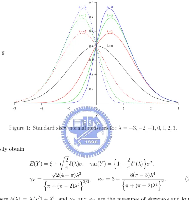
(9) thus present how to compute the ML estimates for the skew normal distribution by using the ECM and ECME algorithms. In Section 3 we show the hierarchical formulation for skew normal mixture models by comprising two latent variables. Based on the model, we derive EM-type algorithms for ML estimation. Meanwhile, the information-based standard errors are also presented. In Section 4 we develop the MCMC sampling algorithm used in simulating posterior distributions to conduct Bayesian inferences. In Section 5 two real examples are illustrated, and in Section 6 we provide some concluding remarks.. 2. The Skew Normal Distribution 2.1. Preliminaries As developed by Azzalini (1985, 1986), a random variable Y follows a univariate skew normal distribution with location parameter ξ, scale parameter σ 2 and skewness parameter λ ∈ R if Y has the following density function: ¶ ¶ µ µ y−ξ y−ξ 2 2 , Φ λ ψ(y | ξ, σ , λ) = φ σ σ σ. (1). where φ(·) and Φ(·) denote the standard normal density function and cumulative distribution function, respectively; then, for brevity, we shall say that Y ∼ SN (ξ, σ 2 , λ). Note that if λ = 0, then the density of Y will be reduced to N (ξ, σ 2 ) density. Figure 1 shows the plots of standard skew normal densities (ξ = 0, σ = 1) for various λ. ³ 2 ´ Lemma 1 If Y ∼ SN (ξ, σ 2 , λ) and X ∼ N ξ, σ 2 , we have 1+λ σ 2 d E(X n ). 1 + λ2 dξ q 2 δ(λ)σE(X n ). (ii) E(Y n+1 ) = ξE(Y n ) + σ 2 d E(Y n ) + π dξ © ªn © ªn−1 © ªn+1 (iii) E Y − E(Y ) = σ 2 d E Y − E(Y ) + nσ 2 E Y − E(Y ) dξ © ªn © ª © ªn q 2 − E(Y ) − ξ E Y − E(Y ) + π δ(λ)σE X − E(Y ) . (i) E(X n+1 ) = ξE(X n ) +. Lemma 1 provides a simple way of obtaining the higher moments without using the moment generating function. With some basic algebraic manipulations, we can. 3.

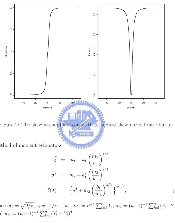
(10) Densities of standard Skew−Normal with various skewnesses 0.7 λ = −3. 0.6. λ=2. λ = − 1 0.5. λ=1. 0.4. λ=0. f(x). λ = −2. λ=3. 0.3. 0.2. 0.1. −3. −2. −1. 0. 1. 2. 3. x. Figure 1: Standard skew normal densities for λ = −3, −2, −1, 0, 1, 2, 3.. easily obtain r. n 2 2 o 2 2 δ(λ)σ, var(Y ) = 1 − δ (λ) σ , E(Y ) = ξ + π π √ 3 8(π − 3)λ4 2(4 − π)λ γY = n o2 , o3/2 , κY = 3 + n 2 2 π + (π − 2)λ π + (π − 2)λ. (2). √ where δ(λ) = λ/ 1 + λ2 , and γY and κY are the measures of skewness and kurtosis, respectively. It is easily shown that γY lies in (−0.9953, 0.9953) and κY in (3, 3.8692). Figure 2 displays γY and κY for different λ. Henze (1986) shows that the odd moments of the standard skew normal variable Z = (Y − ξ)/σ have the following expressions: r E(Z. 2k+1. )=. k X j!(2λ)2j 2 2 −(k+0.5) −k , λ(1 + λ ) 2 (2k + 1)! (2j + 1)!(k − j)! π j=0. while the even moments coincide with those of standard normal, as Z 2 ∼ χ21 . From (2), Arnold, Beaver, Groeneveld and Meeker (1993) show the following 4.

(11) 3.8. 1.0. kurtosis. 3.2. 3.4. 3.6. 0.5 0.0. skewness. -0.5. 3.0. -1.0. -40. -20. 0. 20. 40. -40. -20. lambda. 0. 20. 40. lambda. Figure 2: The skewness and kurtosis of the standard skew normal distribution.. method of moment estimators: µ ξ˜ = m1 − a1. m3 b1. ¶1/3 ,. ¶2/3 m3 , σ ˜ = m2 + b1 µ ¶2/3 o n −1/2 b1 2 ˜ , δ(λ) = a1 + m2 m3. µ. 2. a21. p. 2/π, b1 = (4/π−1)a1 , m1 = n−1 P and m3 = (n − 1)−1 ni=1 (Yi − Y¯i )3 .. where a1 =. Pn i=1. Yi , m2 = (n−1)−1. (3) Pn. ¯ 2 i=1 (Yi − Yi ). 2.2. Parameter estimation using EM-type algorithms We show two faster extensions of the EM algorithm (Dempster, Laird and Rubin, 1977), the ECM algorithm (Meng and Rubin, 1993) and the ECME algorithm (Liu and Rubin, 1994), for the ML estimation of the skew normal distribution. In order 5.

(12) to represent the skew normal model in an incomplete data framework, we extend the result of Azzalini (1986, p. 201) and Henze (1986, Theorem 1) to show that if Yj ∼ SN (ξ, σ 2 , λ), then Yj = ξ + δ(λ)τj +. p. 1 − δ 2 (λ)Uj ,. (4). with τj ∼ T N (0, σ 2 )I{τj > 0},. Uj ∼ N (0, σ 2 ),. where τj and Uj are independent, and T N (·, ·) denotes the truncated normal distribution, and I{·} represents an indicator function. Letting Y = (Y1 , . . . , Yn ) and τ = (τ1 , . . . , τn ), the complete-data log-likelihood of θ = (ξ, σ 2 , λ) given (Y , τ ) is ³ ´ n `c (θ) = −n log(σ 2 ) − log 1 − δ 2 (λ) 2 Pn Pn Pn 2 2 j=1 (yj − ξ) j=1 τj (yj − ξ) + j=1 τj − 2δ(λ) ³ ´ . (5) − 2σ 2 1 − δ 2 (λ) Obviously, the posterior distribution of τj is τj |Yj = yj ∼ T N (µτj , στ2 )I{τj > 0}, where µτj = δ(λ)(yj − ξ) and στ = σ. p. (6). 1 − δ 2 (λ).. Lemma 2 Let X ∼ T N (µ, σ 2 )I{a1 < x < a2 } be a truncated normal distribution with the following density function: ¾ ½ o−1 1 1 2 √ exp − 2 (x − µ) , f (x|µ, σ ) = Φ(α2 ) − Φ(α1 ) 2σ 2πσ 2. n. a 1 < x < a2 ,. where αi = (ai − µ)/σ, i = 1, 2. Then ³ 2 2 ń Φ(α − σt) − Φ(α − σt) o 2 1 σ . (i) MX (t) = exp µt + 2t Φ(α2 ) − Φ(α1 ) (ii) E(X) = µ − σ. φ(α2 ) − φ(α1 ) . Φ(α2 ) − Φ(α1 ). (iii) E(X 2 ) = µ2 + σ 2 − σ 2. φ(α2 ) − φ(α1 ) α2 φ(α2 ) − α1 φ(α1 ) . − 2µσ Φ(α2 ) − Φ(α1 ) Φ(α2 ) − Φ(α1 ). 6.

(13) By Lemma 2, we have E(τj |yj ) = µτj +. φ(µτj /στ ) φ(µτj /στ ) µτ στ . στ and E(τj2 |yj ) = µ2τj + στ2 + Φ(µτj /στ ) j Φ(µτj /στ ). Then we have the following ECM algorithm: E-step: Calculating the conditional expectation of (5) at the kth iteration yields ½ ³ ˆ(k) ´¾ (k) yj − ξ ˆ φ λ σ ˆ (k) (k) (k) ˆτ(k) , sˆ1j = E ˆ (k) (τj |yj ) = µ ˆ τj + ½ ³ y − ξˆ(k) ´¾ σ θ ˆ (k) j Φ λ σ ˆ (k) ½ ³ ˆ(k) ´¾ (k) yj − ξ ˆ φ λ σ ˆ (k) (k) 2 (k)2 (k)2 ˆτ(k) σ ˆτ(k) , ˆ τj + σ ˆτ + ½ sˆ2j = E ˆ (k) (τj |yj ) = µ j ³ y − ξˆ(k) ´¾ µ θ ˆ (k) j Φ λ σ ˆ (k) (k). (k). where µ ˆτj , σ ˆτ. ˆ (k) , are µτj and στ in (6) with ξ, σ and λ replaced by ξˆ(k) , σ ˆ (k) and λ. respectively. CM-steps CM-step 1: Update ξˆ(k) by ξˆ(k+1). 1 = n. Ã n X. ˆ (k) ) yj − δ(λ. j=1. n X. ! (k) sˆ1j. .. j=1. (k). CM-step 2: Update σ ˆ 2 by P Pn (k) (k) ˆ (k) ) Pn (yj − ξˆ(k+1) )ˆ s1j + nj=1 (yj − ξˆ(k+1) )2 ˆ2j − 2δ(λ j=1 j=1 s 2(k+1) . σ ˆ = ¡ ¢ ˆ (k) ) 2n 1 − δ 2 (λ (k+1) ˆ (k+1) as the solution of the , obtaining λ CM-step 3: Fix ξ = ξˆ(k+1) and σ 2 = σ ˆ2. following equation: nˆ σ. 2(k+1). n X ¡ ¢ (k) 2 2 δ(λ) 1 − δ (λ) + δ (λ) (yj − ξˆ(k+1) )ˆ s1j j=1. −δ(λ). n X j=1. (k). sˆ2j − δ(λ). n X. (yj − ξˆ(k+1) )2 = 0.. j=1. For the ECME algorithm, the E-step and the first two CM steps are the same as ECM, while the CM-Step 3 of ECM is modified as the following CML-step. 7.

(14) ˆ (k) by optimizing the constrained log-likelihood function, i.e., CML-step: Update λ ˆ (k+1). λ. ¾ ½ ³ yj − ξˆ(k+1) ´ . = argmax log Φ λ σ ˆ (k+1) λ j=1 n X. The maximization in the CML-step needs a one-dimensional search, which can be easily solved by the function “optim” embedded in the statistical package “R”. As noted by Liu and Rubin (1994), the ECME has a faster convergence rate than the ECM algorithm. Lemma 3 If Z ∼ SN (0, 1, λ), then ¾ q ½ φ(λZ) 2√ 1 . = π (i) E Φ(λZ) 1 + λ2 ¾ ½ 2k+1 φ(λZ) = 0, k = 0, 1, 2, . . .. (ii) E Z Φ(λZ) ¾ q ½ λ ¢ . 2¡ 2 φ(λZ) = π (iii) E Z 3/2 Φ(λZ) 1 + λ2 The method of moments estimators in (3) can provide good initial values. Applying Lemma 3, the Fisher information I(ξ, σ, λ) can be easily obtained. The results are shown in the following lemma. The standard errors of ML estimates can be computed by taking the square root of the corresponding diagonal elements of ˆσ ˆ I −1 (ξ, ˆ , λ). Lemma 4 The Fisher information for θ = (ξ, σ 2 , λ) is Ã I(θ) = E −. ∂ 2 `(θ|y) ∂θ∂θ >. . !. Iξξ. Iξσ2. Iξλ. .   =  Iξσ2 Iσ2 σ2 Iσ2 λ  , Iξλ Iσ2 λ Iλλ. 8. (7).

(15) where ¶ n ∂ 2 `(θ|y) (1 + λ2 a0 ), = Iξξ = E − σ2 ∂ξ 2 ! Ãr ¶ µ 2 2 λ + 2λ3 n ∂ `(θ|y) + λ2 a1 , = 3 Iξσ2 = E − π (1 + λ2 )3/2 2σ ∂ξ∂σ 2 ¶ µ ¶ µ 2 1 n 2 ∂ `(θ|y) − λa1 , = Iξλ = E − σ π (1 + λ2 )3/2 ∂ξ∂λ ¶ µ ¶ µ 2 1 2 n ∂ `(θ|y) = 4 1 + λ a2 , Iσ 2 σ 2 = E − 2 2σ ∂σ 2 ¶ µ 2 nλ ∂ `(θ|y) = − 2 a2 , Iσ2 λ = E − 2 2σ ∂σ ∂λ ¶ µ 2 ∂ `(θ|y) = na2 . Iλλ = E − ∂λ2 ³ ¡ ¢2 ´ k Note that the quantities ak = E Z φ(λZ)/Φ(λZ) , (k = 0, 1, 2) need to. µ. be evaluated numerically. Based on the large sample theorem, the standard errors 2 ˆ ML = (ξˆML , σ ˆ ML ) can be computed by taking estimates for the ML estimates θ ˆML ,λ ˆ ML ). the square root of the corresponding diagonal elements of J−1 (θ. 3. The Skew Normal Mixtures 3.1. The model We consider a finite mixture model in which a set of independent data Y1 , . . . , Yn are from a g-component mixture of skew normal densities f (yj | ω, Θ) =. g X. ωi ψ(yj | ξi , σi2 , λi ),. (8). i=1. where ω = (ω1 , . . . , ωg ) are the mixing probabilities which are constrained to be non-negative and sum to unity and Θ = (θ 1 , . . . , θ g ) with θ i = (ωi , ξi , σi2 , λi ) being the specific parameters for component i. We introduce a set of latent component-indicators Z j = (Z1j , . . . , Zgj ), j = 1, . . . , n, whose values are a set of binary variables with ( 1 if Y j belongs to group k, Zkj = 0 otherwise, 9.

(16) and. Pg i=1. Zij = 1. Given the mixing probabilities ω, the component-indicators. Z 1 , . . . , Z n are independent, with multinomial densities z. z. f (z j ) = ω11j ω22j · · · (1 − ω1 − · · · − ωg )zgj .. (9). We shall write Z j ∼ M N (1; ω1 , . . . , ωg ) to denote Z j with density (9). From (4), a hierarchical model for skew normal mixtures can thus be written as ³ ¡ ¢ ´ Yj | τj , Zij = 1 ∼ N ξi + δ(λi )τj , 1 − δ 2 (λi ) σi2 , τj | Zij = 1 ∼ T N (0, σi2 )I(τj > 0), Z j ∼ M N (1; ω1 , . . . , ωg ). (j = 1, . . . , n).. (10). 3.2. Maximum likelihood estimation As in (6), we have τj | Yj = yj , Zij = 1 ∼ T N (µτij , στ2i )I{τj > 0}, where µτij = δ(λi )(yj − ξi ),. στi = σi. p. 1 − δ 2 (λi ).. From (10), the complete-data log-likelihood function is ( g n X ³ ´ X 1 `c (θ) = Zij log(ωi ) − log(σi2 ) − log 1 − δ 2 (λi ) 2 j=1 i=1 ) τj2 − 2δ(λi )τj (yj − ξi ) + (yj − ξi )2 ³ ´ . − 2σi2 1 − δ 2 (λi ). (11). (12). Letting zîj = E ˆ (k) (Zij | Y ), sˆ1ij = E ˆ (k) (Zij τj | Y ) and sˆ2ij = E ˆ (k) (Zij τj2 | Θ Θ Θ Y ) be the necessary conditional expectations of (12), we obtain (k) zîj. (k). (k). (k). (k). ωi ψ(yj | ξi , σi2 , λi ). , (k) (k) 2(k) , λ(k) ) ωm ψ(yj | ξm , σm m ½  ³ ˆ(k) ´¾  yj −ξi (k) ˆ φ λ (k)   σ î (k) (k) (k) , ¾ ½ µ ˆ = zîj  + σ ˆ ´ ³ τ τ ij i   ˆ(k) y − ξ (k) j i ˆ Φ λ (k). = Pg. (13). m=1. (k). sˆ1ij. i. 10. σ î. (14).

(17) and   (k)2 2 (k) (k) ˆτij + σ sˆ2ij = zîj  ˆτ(k) + i µ. ½ ³ ˆ(k) ´¾ yj −ξi (k) ˆ φ λ (k). .  σ î , ½ ˆ(k) ˆτ(k) ³ ˆ(k) ´¾ µ τij σ i  y − ξ (k) j i ˆ Φ λ (k) i. (15). σ î. (k) (k) where µ ˆτij , σ ˆτi are µτij and στi in (11) with ξ, σ and λ replaced by ξˆ(k) , σ ˆ (k) and ˆ (k) , respectively. λ. The ECM algorithm is as follows: ˆ (k) , compute zˆ(k) , sˆ(k) and sˆ(k) for i = 1, . . . , g and j = E-step: Given Θ = Θ ij 1ij 2ij 1, . . . , n, using (13), (14) and (15). CM-step 1: Calculate. n. (k+1) ω î. 1 X (k) zˆ . = n j=1 ij. CM-step 2: Calculate ˆ (k) ) Pn sˆ(k) − δ(λ i j=1 1ij . Pn (k) z ˆ j=1 ij. Pn (k+1) ξî. (k) îj yj j=1 z. =. CM-step 3: Calculate Pn (k+1) σ î2. =. j=1. (k) ˆ (k) ) Pn sˆ(k) (yj − ξˆ(k+1) ) + Pn zˆ(k) (yj − ξˆ(k+1) )2 sˆ2ij − 2δ(λ i i i j=1 ij j=1 1ij . ¡ (k) ¢ Pn (k) 2 ˆ 2 1 − δ (λi ) z ˆ j=1 ij. (k+1) (k+1) ˆ (k+1) (i=1,. . . ,g) as the î2 , obtaining λ and σi2 = σ CM-step 4: Fix ξi = ξî i. solution of the following equation: ¡. (k+1) σ î2 δ(λi ). −δ(λi ). n X. n n X ¢X (k+1) (k) (k) 2 )ˆ s1ij 1 − δ (λi ) (yj − ξî zîj + δ (λi ) 2. (k). sˆ2ij − δ(λi ). j=1. j=1 n X. j=1. (k) (k+1) 2 zîj (yj − ξî ) = 0.. j=1. ECME is identical to ECM except for the CM-Step 4 of ECM, which can be modified by the following CML-Step:. 11.

(18) ˆ (k) as CML-step: Let λ = (λ1 , . . . , λg ) and update λ (k+1). ˆ λ. = argmax λ1 ,...,λg. n X j=1. log. µX g. (k+1) ψ(yj ω î. |. (k+1) , ξî. (k+1) σ î2 ,. ¶ λi ) .. i=1. We remark here that if the skewness parameters λ1 , . . . , λg are assumed to be identical, we shall use ECME since it is more efficient than ECM. Otherwise, the CML-step becomes a non-trivial high dimensional optimization problem while using the CM-step 4 can avoid the complication. 3.3. Standard errors We let I o (Θ | y) = −∂ 2 `(Θ | Y )/∂Θ∂Θ> be the observed information matrix for the mixture model (8). Under some regularity conditions, the covariance matrix ˆ can be approximated by the inverse of I o (Θ ˆ | y). We follow of ML estimates Θ Basford, Greenway, McLachlan and Peel (1997) to evaluate ˆ | y) = I o (Θ. n X. ˆsj ˆs> j ,. (16). j=1. where ˆsj = ∂ log. nP. g i=1. o ¯ ωi ψ(yj | ξi , σi2 , λi ) /∂Θ¯. ˆ . Θ=Θ Corresponding to the vector of all unknown 4g −1 parameters in Θ, we partition. ˆsj (j = 1, . . . , n) as ˆsj = (ˆ sj,ω1 , . . . , sˆj,ωg−1 , sˆj,ξ1 , . . . , sˆj,ξg , sˆj,σ1 , . . . , sˆj,σg , sˆj,λ1 , . . . , sˆj,λg )> . The elements of ˆsj are given by ˆg ) ˆ r ) − ψ(yj | ξˆg , σ ˆg2 , λ ψ(yj | ξˆr , σ ˆr2 , λ (r = 1, . . . , g − 1), Pg 2 ˆ î , σ , λ ) ω ˆ ψ(y | ξ ˆ i i j i i=1 (µ ª © ¶ ¶ µ ˆ 2ˆ ωr φ (yj − ξr )/ˆ σr yj − ξˆr yj − ξˆr ˆ − Φ λr = P î) σ ˆr σ ˆr ˆ i ψ(yj | ξî , σ î2 , λ σ ˆr2 gi=1 ω ) µ ˆr ¶ y − ξ j ˆr ˆr φ λ (r = 1, . . . , g), −λ σ ˆr. sˆj,ωr = sˆj,ξr. 12.

(19) sˆj,σr. sˆj,λr. ( ˆr ) (yj − ξˆr )2 1 ω ˆ r ψ(yj | ξˆr , σ ˆr2 , λ + − = Pg î) σ ˆr3 σ ˆr ˆ i ψ(yj | ξî , σ î2 , λ i=1 ω ¢) ¢ ¡ ¡ ˆ r (yj − ξˆr )/ˆ ˆ r (yj − ξˆr )φ (yj − ξˆr )/ˆ σr σr φ λ 2ˆ ωr λ (r = 1, . . . , g), − P î) ˆ i ψ(yj | ξî , σ î2 , λ σ ˆr3 gi=1 ω o n ¶ µ ˆ ˆ λ (y − ξ )/ˆ σ φ 2 ˆr ) r j r r yj − ξˆr ω ˆ r ψ(yj | ξˆr , σ ˆr , λ o (r = 1, . . . , g). n = Pg 2 ˆ î , σ σ ˆ ˆ ˆ r , λ ) ω ˆ ψ(y | ξ ˆ i i j λ (y − ξ )/ˆ σ Φ i i=1 r j r r. The information-based approximation (16) is asymptotically applicable. However, it may not be reliable unless the sample size is large. It is common in practice to use the bootstrap approach (Efron and Tibshirani, 1986) as an alternative Monte ˆ via generating a sufficient number of bootstrap samCarlo approximation of cov(Θ) ples. The bootstrap method may provide more accurate stand error estimates than (16). However, it requires enormous computational burden.. 4. Bayesian Modelling For Skew Normal Mixtures We consider a Bayesian approach where Θ is regarded as random with a prior distribution that reflects our degree of belief in different values of these quantities. Since fully non-informative prior distributions are not permissible in the mixture context, the prior distributions chosen are weakly informative subject to vague prior knowledge and avoid causing nonintegrable posterior distributions. The prior distributions for model (8) are of the forms ξi ∼ N (η, κ−1 ) (i = 1, . . . , g), σi−2 | β ∼ Ga(α, β) (i = 1, . . . , g), β ∼ Ga(ν1 , ν2 ), δ(λi ) ∼ U (−1, 1) (i = 1, . . . , g), ω ∼ D(h, . . . , h), with the restriction ξ1 < · · · < ξg .. (17). In (17), β is an unknown hyperparame-. ter, (η, κ, α, ν1 , ν2 , h) are known (data-dependent) constants, Ga(α, β) denotes the gamma distribution with mean α/β and variance α/β 2 , U (−1, 1) denotes the continuous uniform distribution on the interval [−1, 1] and D(h, . . . , h) stands for the. 13.

(20) Dirichlet distribution with the density function ³ X ´h−1 Γ(gh) h−1 h−1 ω · · · ωg−1 1 − ωi . Γ(h)g 1 i=1 g−1. For the values of (η, κ, α, ν1 , ν2 , h), we follow Richardson and Green (1997) by letting η be equal to the midpoint of the observed interval and κ−1 = R2 , where R is the range and setting α = 2, ν1 = 0.2, ν2 = 100ν1 /(αR2 ) and h = 1. Given Θ = Θ(k) , the MCMC sampling scheme at the (k + 1)th iteration consists of the following steps: (k+1). Step 1: Sample Z j. (j = 1, . . . , n) from M N (1; ω1∗ , . . . , ωg∗ ), where (k). ωi∗. = Pg. (k). (k). (k). ωi ψ(yj | ξi , σi2 , λi ) (k). (k). (k). 2(k) m=1 ωm ψ(yj | ξm , σm , λm ). (i = 1, . . . , g).. (k+1). Step 2: Given Zij = 1, sample τj (j = 1, . . . , n) from ³ ´ (k) ¡ (k) ¢ (k) (k) T N δ(λi )(yj − ξi ), σi2 1 − δ 2 (λi ) I{τj > 0}. Step 3: Sample β (k+1) from Ga(ν1 + gα, ν2 + (k+1). Step 4: Sample ω (k+1) from D(h+n1. Pg. (k). i=1. σi−2 ).. (k+1). , . . . , h+ng. (k+1). ), where ni. =. Pn j=1. (k+1). Zij. (k+1). Step 5: Given Zij = 1, sample ξi from Ã ¾−1 ! ½ (k+1) n (k+1) i , +κ N µξi , ¡ (k) ¢ 2(k) 1 − δ 2 (λi ) σi where Pn (k+1). µξi. =. (k+1). j=1 Zij. (k). (k+1). Step 6: Given Zij = 1, sample σi−2 b =. n nX. (k+1) 2(k+1) τj. Zij. Pn. (k). j=1 Zij. ¡ (k) ¢ 1 − δ 2 (λi ). ¡ ¢ (k+1) from Ga α + ni , β (k+1) + b , where (k). − 2δ(λi ). j=1. +. (k+1) (k+1) τj. + κησi2 ¡ (k) (k) ¢ (k+1) ni + κσi2 1 − δ 2 (λi ). yj − δ(λi ). n X. (k+1). Zij. (k+1). τj. (k+1). (yj − ξi. j=1 n X. o n ¡ ¢o (k+1) (k+1) 2 2 (k) Zij (yj − ξi ) / 2 (1 − δ (λi ) .. j=1. 14. ). .. ..

(21) ¡ (k+1) (k+1) ¢ Step 7: Sample δ (k+1) = δ(λ1 ), . . . , δ(λg ) via the Metropolis Hastings (MH) algorithm (Hastings, 1970) from # (k+1) " ½ g (k+1) (k+1) ¾ Zij n Y ¡ ¢ Y ¡ ¢ 2δ(λ )τ (y − ξ ) i j j −1/2 i ¡ ¢ . f δ ∝ 1 − δ 2 (λi ) exp 2(k) 2 1 − δ (λ ) 2σ i i i=1 j=1 To elaborate on Step 7 of the above algorithm, we transform δ(λi ) to δ ∗ (λi ) = ©¡ ¢ ¡ ¢ª log 1 + δ(λi ) / 1 − δ(λi ) and then apply the M-H algorithm to the following function:. g ¡ ∗¢ ¡ ¢Y ∗ g δ = f δ(δ ) Jδ∗ (λi ) , i=1. ¢2 ¡ ¢ ¡ ∗ ∗ where δ ∗ = δ ∗ (λ1 ), . . . , δ ∗ (λg ) , and Jδ∗ (λi ) = 2eδ (λi ) / 1 + eδ (λi ) is the Jacobin of transformation from δ(λi ) to δ ∗ (λi ). A g-dimensional multivariate normal distribution with mean δ ∗. (k). (k). and covariance matrix c2 Σ ∗ is chosen as the proposal δ √ distribution, where the scale c ≈ 2.4/ g, as suggested in Gelman, Roberts and Gilks (1995). The value of Σ. (k). can be estimated by the inverted sample informaδ∗ (k) tion matrix given y and Θ = Θ . Having obtained δ ∗ from the M-H algorithm, we ∗. ∗. transform it back to δ by δ(λi ) = (eδ (λi ) − 1)/(eδ (λi ) + 1) (i = 1, . . . , g), and then p transform δ(λi ) back to λi by δ(λi )/ 1 − δ 2 (λi ). To avoid the label-switching problem and slow stabilization of the Markov chain, our initial values Θ(0) are chosen to (0). (0). be dispersed around the ML estimates with the restriction ξ1 < · · · < ξg .. 5. Examples 5.1. The enzyme data We first carry out our methodology for the enzyme data set with n = 245 observations. The data was first analyzed by Bechtel, Bonaita-Pellieé, Poisson, Magnette and Bechtel (1993), who identified a mixture of skew distributions by the maximum likelihood techniques of Maclean, Morton, Elston and Yee (1976). Richardson and Green (1997) provide the reversible jump MCMC approach for the univariate normal mixture models with an unknown number of components and identify the most possible values of g to be between 3 and 5. We fit the data to the two-component skew normal mixture model f (y) = ωψ(y|ξ1 , σ12 , λ1 ) + (1 − ω)ψ(y|ξ2 , σ22 , λ2 ). 15. (18).

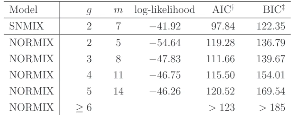
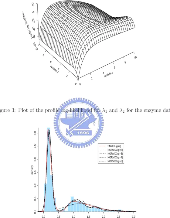
(22) The ECM algorithm was run with various starting values and was checked for convergence. The resulting ML estimates and the corresponding standard errors are listed in Table 1. We found that the standard error for λ2 is relatively large. This is due to the fact that the log-likelihood function can be fairly flat near the ML estimates of the shape parameter of the skew normal components. We have shown this by plotting the profile log-likelihood function of (λ1 , λ2 ) in Figure 3. For comparison purposes, we also fit the data to the normal mixture models (λ1 = λ2 = 0) with g = 2 − 5 components. The log-likelihood maximum and two information-based criteria, AIC (Akaike, 1973) and BIC (Schwarz, 1978), are displayed in Table 2. As expected, the fitting of a skew normal mixture model is superior to normal mixtures since it has the largest log-likelihood with parsimonious parameters as well as the smallest AIC and BIC. A histogram of the data overlaid with various fitted mixture densities is displayed in Figure 4. Table 1: Estimated parameter values and the corresponding standard errors (SE) for model (18) with the enzyme data. ω. ξ1. ξ2. σ1. σ2. λ1. λ2. Estimate. 0.6240 0.0949. 0.7802. 0.1331 0.7150. 3.2780. 6.6684. SE. 0.0310 0.0107. 0.0516. 0.0109. 0.9467. 3.9640. 0.0607. Table 2: A comparison of log-likelihood maximum, AIC and BIC for the fitted skew normal mixture (SNMIX) model and normal mixture (NORMIX) model for the enzyme data. The number of parameters is denoted by m.. †. Model. g. m. log-likelihood. AIC†. BIC‡. SNMIX. 2. 7. −41.92. 97.84. 122.35. NORMIX. 2. 5. −54.64. 119.28. 136.79. NORMIX. 3. 8. −47.83. 111.66. 139.67. NORMIX. 4. 11. −46.75. 115.50. 154.01. NORMIX. 5. 14. −46.26. 120.52. 169.54. NORMIX. ≥6. > 123. > 185. © ª AIC=−2(log-likelihood−m); ‡ BIC=−2 log-likelihood−0.5m log(n) .. 16.

(23) 20 0. ood. -80. ih kel g-li e lo l i f Pro 0 -20 -60 -4. 10 8. 10 6. 8. lam. 6. bd 4 a.2. 4. 2. 2 0. lam. .1 bda. 0. 2.5. 3.0. Figure 3: Plot of the profile log-likelihood for λ1 and λ2 for the enzyme data.. 0.0. 0.5. 1.0. density 1.5. 2.0. SNMIX (g=2) NORMIX (g=2) NORMIX (g=3) NORMIX (g=4) NORMIX (g=5). 0.0. 0.5. 1.0. 1.5. 2.0. 2.5. 3.0. y. Figure 4: Histogram of the enzyme data overlaid with a ML-fitted two-component skew normal mixture (SNMIX) distribution and various ML-fitted g-component normal mixture (NORMIX) distributions (g = 2 − 5). 17.

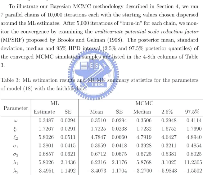
(24) 5.2. The faithful data As another example, we consider the Old Faithful Geyser data taken from Silverman (1986). It consists of 272 eruption lengths (in minutes) of the Old Faithful Geyser in the Yellowstone National Park, Wyoming, USA. The data appear to be bimodal with asymmetrical components. We fit a two-component skew mixture normal model (18) by analogy with the previous example. The ML estimates and the corresponding standard errors are reported in the second and third columns of Table 3, respectively. To illustrate our Bayesian MCMC methodology described in Section 4, we ran 7 parallel chains of 10,000 iterations each with the starting values chosen dispersed around the ML estimates. After 5,000 iterations of “burn-in” for each chain, we monitor the convergence by examining the multivariate potential scale reduction factor (MPSRF) proposed by Brooks and Gelman (1998). The posterior mean, standard deviation, median and 95% HPD interval (2.5% and 97.5% posterior quantiles) of the converged MCMC simulation samples are listed in the 4-8th columns of Table 3. Table 3: ML estimation results and MCMC summary statistics for the parameters of model (18) with the faithful data. Parameter. MCMC. ML Estimate. SE. Mean. SE. Median. 2.5%. 97.5%. ω. 0.3487. 0.0294. 0.3510. 0.0294. 0.3506. 0.2948. 0.4114. ξ1. 1.7267. 0.0291. 1.7225. 0.0238. 1.7232. 1.6752. 1.7690. ξ2. 5.8026. 0.0511. 4.7847. 0.0660. 4.7919. 4.6427. 4.8940. σ1. 0.3801. 0.0415. 0.3959. 0.0418. 0.3928. 0.3211. 0.4854. σ2. 0.6857. 0.0621. 0.6712. 0.0675. 0.6725. 0.5381. 0.8025. λ1. 5.8026. 2.1436. 6.2316. 2.1176. 5.8768. 3.1025. 11.2305. λ2. −3.4951. 1.1492. −3.4073. 1.1704. −3.2700. −5.9843. −1.5502. Figure 5 displays the convergence diagrams and histograms of the posterior samples of the parameters. It is evident that the shape of the posterior distribution of λ1 is skewed to the right, while the shape of the posterior distribution of λ2 is skewed 18.

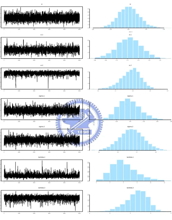
(25) to the left. It is interesting to note that the posterior distributions of the parameters (λ1 , λ2 ) which regulate the skewness are skewed as well. Finally, we compare the ML-fitted normal mixture density with the fitted skew normal mixture densities via ML and Byesian methods based on graphical visualization. The ML density estimation for normal and skew normal mixtures densities together with Bayesian predictive density are shown in Figure 6(a). We have also plotted the comparison of fitted and empirical cumulative density functions (CDFs) in Figure 6(b). Obviously, the ML and Bayesian methods are quite comparable for the data. However, the appropriateness of density fitting for skew normal mixtures is clearly better than for normal mixtures. Furthermore, the CDFs of the skew normal mixtures track closer to the real data.. 19.

(26) w. 0. 0.25. 2. 0.30. 4. 6. 0.35. 8. 0.40. 10. 12. 0.45. w. 0. 1000. 2000. 3000. 4000. 5000. 0.25. 0.30. 0.35. 0.40. 0.45. par[, 1]. xi.1. 0. 1.65. 5. 1.70. 1.75. 10. 1.80. 15. 1.85. xi.1. 0. 1000. 2000. 3000. 4000. 5000. 1.66. 1.68. 1.70. 1.72. 1.74. 1.76. 1.78. xi.2. 0. 4.2. 2. 4.4. 4. 4.6. 4.8. 6. 5.0. xi.2. 0. 1000. 2000. 3000. 4000. 5000. 4.6. 4.7. 4.8. 4.9. 5.0. sigma.1. 0. 0.3. 2. 4. 0.4. 6. 0.5. 8. 0.6. sigma.1. 0. 1000. 2000. 3000. 4000. 5000. 0.25. 0.30. 0.35. 0.40. 0.45. 0.50. 0.55. sigma.2. 0. 0.4. 1. 0.5. 2. 0.6. 3. 0.7. 4. 0.8. 5. 0.9. 6. sigma.2. 0. 1000. 2000. 3000. 4000. 5000. 0.5. 0.6. 0.7. 0.8. lambda.1. 0. 0.0. 5. 0.05. 10. 0.10. 15. 0.15. 20. 0.20. 25. lambda.1. 0. 1000. 2000. 3000. 4000. 5000. 2. 4. 6. 8. 10. 12. lambda.2. 0.0. -10. 0.1. -8. -6. 0.2. -4. -2. 0.3. 0. lambda.2. 0. 1000. 2000. 3000. 4000. 5000. -8. -6. -4. -2. 0. Figure 5: Convergence diagrams and histograms of the posterior sample of the parameters for model (18) with the faithful data.. 20.

(27) 0.8. (a). 0.0. 0.2. density 0.4. 0.6. SNMIX (Bayesian) SNMIX (ML) NORMIX (ML). 1.3. 2.0. 3.0. 4.0. 5.0. y. 1.0. (b). 0.0. 0.2. 0.4. CDFs. 0.6. 0.8. Empirical SNMIX (Bayesian) SNMIX (ML) NORMIX (ML). 2. 3. 4. 5. y. Figure 6: (a)Histogram of the faithful data overlaid with densities based on two fitted two-component skew normal mixture (SNMIX) distributions (ML and Bayesian), and a ML-fitted two-component normal mixture (NORMIX) distribution; (b)Empirical CDF of the faithful data overlaid with CDFs based on two fitted two-component SNMIX distributions (ML and Bayesian) and a ML-fitted two-component NORMIX distribution.. 21.

(28) 6. Conclusion We have proposed and illustrated ML and Bayesian density estimations for finite mixture modelling using the skew normal distribution. The key contributions lie in the development of computational techniques for the hierarchical skew normal mixtures. We provide EM-type algorithms for calculating the ML estimates and a workable MCMC algorithm for sampling the posterior distributions in the Bayesian paradigm. In our illustrated examples, it is quite appealing that the skew normal mixtures can provide more appropriate density estimation than normal mixtures based on information-based criteria and graphical visualization. Future work on extensions includes generalizations to mixture of multivariate skew normal distributions (e.g., Azzalini and Dalla Valle, 1996 and Gupta, González-Far´ıas and Dom´ınguez-Monila, 2004) and offering techniques to model the number of components and the mixture components parameters jointly.. Appendix A. Proof of Lemma 1 (i) √ 2 ¡ 1 + λ2 ¢ 1 + λ (x − ξ) dx, φ E(X n ) = xn σ σ √ √ Z 2 2 ¡ 1 + λ2 ¢ 1+λ d n 1+λ n (x − ξ) dx φ (x − ξ)x E(X ) = 2 σ σ σ dξ 2 2 1+λ 1+λ E(X n ), E(X n+1 ) − ξ = 2 σ2 σ σ2 d n+1 n E(X n ). E(X ) = ξE(X ) + 2 1 + λ dξ. √. Z. (ii). Z n. E(Y ) =. 2 ¡y − ξ ¢ ¡ y − ξ ¢ dy, Φ λ yn φ σ σ σ. 22.

(29) Z λ n 2 ¡y − ξ ¢ ¡ y − ξ ¢ y − ξ n 2 ¡y − ξ ¢ ¡ y − ξ ¢ dy φ λ y φ dy − Φ λ y φ 2 σ σ σ σ σ σ σ σ Z y − ξ¢ 1 n ¡√ E(Y n+1 ) ξE(Y n ) 2λ √ dy y φ 1 + λ2 − − = 2 2 2 σ σ σ σ 2π σ E(Y n+1 ) ξE(Y n ) 2λ 1 E(X n ). − 2√ √ − = 2 2 2 σ σ σ 2π 1 + λ. d E(Y n ) = dξ. Z. Hence, d E(Y n+1 ) = ξE(Y n ) + σ 2 E(Y n ) + dξ. r. 2 δ(λ)σE(X). π. (iii) ¡. ¢n d ¡ E Y − E(Y ) dξ. Z. ¢n 2 ¡ y − ξ ¢ ¡ y − ξ ¢ dy, Φ λ φ y − E(y) σ σ σ Z ¢ 2 ¡y − ξ ¢ ¡ y − ξ ¢ ¡ ¢n−1 ¡ d dy Φ λ E(Y ) φ = − n Y − E(Y ) σ σ σ dξ Z ¢n 2 ¡ y − ξ ¢ ¡ y − ξ ¢ y − ξ¡ dy Φ λ φ Y − E(Y ) + σ σ σ σ2 Z ¡ ¢n λ 2 ¡ y − ξ ¢ ¡ y − ξ ¢ dy φ λ φ Y − E(Y ) − σ σ σσ ¡ ¢n−1 = −nE Y − E(Y ) Z ¢n+1 2 ¡ y − ξ ¢ ¡ y − ξ ¢ 1 ¡ dy Φ λ φ E Y − E(Y ) + σ σ σ σ2 Z ¡ ¢n y − ξ 2 ¡ y − ξ ¢ ¡ y − ξ ¢ dy Φ λ φ Y − E(Y ) + σ σ σ2 σ Z ¡ ¢n λ 2 1 ¡√ y − ξ¢ √ φ 1 + λ2 dy Y − E(Y ) − σ σ σ 2π ¢n+1 ¡ ¢n−1 1 ¡ = −nE Y − E(Y ) + 2 E Y − E(Y ) σ r ¢n ¡ ¢ ¡ ¢n 1 ¡ 2 1 δ(λ) E X − E(Y ) . + 2 E(Y ) − ξ E Y − E(Y ) − σ π σ. ¢n = E Y − E(Y ). ¡. Hence, ¢n ¡ ¢n−1 ¡ ¢n+1 d ¡ E Y − E(Y ) = σ 2 E Y − E(Y ) + nσ 2 E Y − E(Y ) dξ r ¡ ¢n ¡ ¢ ¡ ¢n 2 δ(λ)σE X − E(Y ) . − E(Y ) − ξ E Y − E(Y ) + π. 23.

(30) B. Proof of Lemma 2 (i) ¡ ¢ MX (t) = E etx =. Z. a2. etx f (x | µ, σ 2 )dx a1 Z a2 ¢ ¡ 1 1 1 1 exp − 2 (x − µ)2 dx etx √ 2σ Φ(α2 ) − Φ(α1 ) a1 2π σ Z a2 2 2 ¢ ¡ 1 ¡ 1 1 σ t ¢ 1 √ exp − 2 [x − (µ + σ 2 t)]2 dx exp µt + 2σ 2 Φ(α2 ) − Φ(α1 ) 2π σ a1 Z α2 −σt 2 2 ¡ 1 ¢ ¡ 1 σ t ¢ 1 √ exp − z 2 dz exp µt + 2 2 Φ(α2 ) − Φ(α1 ) 2π α1 −σt 2 2¢ ¡ σ t Φ(α2 − σt) − Φ(α1 − σt) . exp µt + Φ(α2 ) − Φ(α1 ) 2. = = = = (ii). σ 2 t2 Φ(α2 − σt) − Φ(α1 − σt) ) M (t) = (µ + σ t) exp (µt + Φ(α2 ) − Φ(α1 ) 2 2 2 φ(α2 − σt) − φ(α1 − σt) σ t , )σ − exp (µt + Φ(α2 ) − Φ(α1 ) 2 φ(α2 ) − φ(α1 ) 0 . E(X) = M (0) = µ − σ Φ(α2 ) − Φ(α1 ) 0. 2. (iii) ¡ σ 2 t2 ¢ Φ(α2 − σt) − Φ(α1 − σt) 00 M (t) = σ 2 exp µt + Φ(α2 ) − Φ(α1 ) 2 ¡ σ 2 t2 ¢ Φ(α2 − σt) − Φ(α1 − σt) +(µ + σ 2 t)2 exp µt + Φ(α2 ) − Φ(α1 ) 2 2 2¢ ¡ φ(α2 − σt) − φ(α1 − σt) σ t σ −(µ + σ 2 t) exp µt + Φ(α2 ) − Φ(α1 ) 2 2 2 ¡ σ t ¢ φ(α2 − σt) − φ(α1 − σt) σ −(µ + σ 2 t) exp µt + Φ(α2 ) − Φ(α1 ) 2 2 2 ¡ σ t ¢ (α2 − σt)φ(α2 − σt) − (α1 − σt)φ(α1 − σt) . σ − exp µt + Φ(α2 ) − Φ(α1 ) 2 φ(α2 ) − φ(α1 ) 00 E(X 2 ) = M (0) = σ 2 + µ2 − µσ Φ(α2 ) − Φ(α1 ) α2 φ(α2 ) − α1 φ(α1 ) φ(α2 ) − φ(α1 ) −σ −µσ Φ(α2 ) − Φ(α1 ) Φ(α2 ) − Φ(α1 ) φ(α2 ) − φ(α1 ) α2 φ(α2 ) − 1αφ (α1 ) . − 2µσ = µ2 + σ 2 − σ Φ(α2 ) − Φ(α1 ) Φ(α2 ) − Φ(α1 ) 24.

(31) C. Proof of Lemma 3 (i) ¡ φ(λZ) ¢ = E Φ(λZ). Z. φ(λz) dz Φ(λz) Z 1 2 2 1 2 1 1 = 2 √ e− 2 z √ e− 2 λ z dz 2π Z 2π 1 1 2 2 e− 2 (1+λ )z dz = π 1 1√ 2π √ = π 1 + λ2 r 1 2 √ . = π 1 + λ2. (ii) ¡ φ(λZ) ¢ = E Z 2k+1 Φ(λZ). 2φ(z)Φ(λz). Z. φ(λz) dz Φ(λz) Z 1 2 2 1 2 1 1 = 2z 2k+1 √ e− 2 z √ e− 2 λ z dz 2π 2π Z 1 1 2 2 z 2k+1 e− 2 (1+λ )z dz = π = 0 (k = 0, 1, 2, · · · ).. (iii) φ(λZ) ¢ = E Z Φ(λZ) ¡. 2. 2φ(z)Φ(λz)z 2k+1. Z. φ(λz) dz Φ(λz) Z 1 2 2 1 2 1 1 = 2z 2 √ e− 2 z √ e− 2 λ z dz 2π 2π Z 1 1 2 2 z 2 e− 2 (1+λ )z dz = π 1 1 1√ 2π √ = 2 π 1 + λ 1 + λ2 r λ 2 . = π (1 + λ)3/2 2φ(z)Φ(λz)z 2. D. Proof of Lemma 4 The log-likelihood function is n. `(θ|y) ∝ −n log(σ) −. n. 1X 2 X z + log(Φ(λzi )), 2 i=1 i i=1 25.

(32) where θ = (ξ, σ 2 , λ), y = (y1 , y2 , . . . , yn ) and zi =. yi − ξ . σ. Let ψ(λzi ) = φ(λzi )/Φ(λzi ), then ∂λzi φ(λzi ) ∂λzi ∂ log(Φ(λzi )) . = ψ(λzi ) = ∂θj Φ(λzi ) ∂θj ∂θj With the following algebraic operations, we have ¶ µ ∂λzi ∂φ(λzi ) 1 ∂ψ(λzi ) 2 − φ (λzi ) Φ(λzi ) = ∂θj ∂θj Φ2 (λzi ) ∂θj ¶ ¶ µ µ ∂λzi ∂λzi 1 2 − φ (λzi ) Φ(λzi ) −λzi φ(λzi ) = ∂θj ∂θj Φ2 (λzi ) ³ ´ ∂λz i = −ψ(λzi ) λzi + ψ(λzi ) ∂θj ∂λzi , = −η(λzi ) ∂θj ³ ´ where η(λzi ) = ψ(λzi ) λzi + ψ(λzi ) . Note that the 1st differentials are ∂λzi λzi λ ∂λzi ∂λzi = zi . = − 2 and =− , 2 ∂λ 2σ σ ∂σ ∂ξ The score vector and Hessian matrix are as follows:     Hξξ Hξσ2 Hξλ sξ     s(θ|Y ) =  sσ2  , and H(θ|Y ) =  Hξσ2 Hσ2 σ2 Hσ2 λ  . Hξλ Hσ2 λ Hλλ sλ The elements of the score vector s(θ|Y ) are n. n. sξ. −1 1 X −1 X ∂`(θ|y) + ψ(λzi )λ 2zi =− = σ σ 2 i=1 ∂ξ i=1 =. n n λX 1X ψ(λzi ), zi − σ i=1 σ i=1 n. n. sσ2. −1λ(yi − ξ) 1 X −1(yi − ξ) X n ∂`(θ|y) + ψ(λzi )λ zi − = − = 4 2 2 2σ 3 σ 2 i=1 2σ ∂σ i=1 n n λ X 1 X 2 n zi ψ(λzi ), z − 2 = − 2+ 2 2σ i=1 2σ i=1 i 2σ n. sλ =. ∂`(θ|y) X = zi ψ(λzi ). ∂λ i=1 26.

(33) The elements of Hessian matrix H(θ|Y ) are Hξξ. n n λ2 X n −λ −n λ X ∂ ∂`(θ|y) η(λzi ), =− 2 − 2 −η(λzi ) = 2 − = σ i=1 σ σ σ i=1 σ ∂ξ ∂ξ. Hξσ2 =. n n n n −λzi λX −λ X 1 X −zi −1 X ∂ ∂`(θ|y) −η(λz ) ψ(λz ) − − z + = i i i 2σ 2 σ i=1 σ i=1 2σ 2 2σ 3 i=1 2σ 3 i=1 ∂σ 2 ∂ξ. n n n λ2 X λ X 1 X zi η(λzi ), ψ(λzi ) − 3 zi + 2 = − 3 2σ i=1 2σ i=1 σ i=1. Hξλ. n n λX 1X ∂ ∂`(θ|y) −η(λzi )zi ψ(λzi ) − =− = σ i=1 σ i=1 ∂λ ∂ξ. = −. n n λX 1X zi η(λzi ), ψ(λzi ) + σ i=1 σ i=1. ∂ ∂`(θ|y) ∂σ 2 ∂σ 2 ¶ µ n n n −λzi λ −λ X 2 3λ X 1 X 2 n z −η(λzi ) zi ψ(λzi ) − 2 2 z + 4 − = σ 2σ 2σ i=1 i 4σ i=1 2σ 4 σ 4 i=1 i. Hσ 2 σ 2 =. n n n λ2 X 2 3λ X 1 X 2 n z η(λzi ), zi ψ(λzi ) − 4 z + 4 − = 4σ i=1 i 4σ i=1 2σ 4 σ 4 i=1 i. Hσ2 λ. n n λ X 1 X ∂ ∂`(θ|y) zi η(λzi )zi zi ψ(λzi ) + 2 =− 2 = 2σ i=1 2σ i=1 ∂λ ∂σ 2 n n λ X 2 1 X z η(λzi ), zi ψ(λzi ) + 2 = − 2 2σ i=1 i 2σ i=1 n. n. Hλλ. X X ∂ ∂`(θ|y) =− zi2 η(λzi ). zi η(λzi )zi = − = ∂λ ∂λ i=1 i=1. In order to simplify symbols, let ³ ´ ³ ´ ak = EY Z k ψ 2 (λZ) , bk = EY Z k ψ(λZ) ,. ³ ´ ck = EY Z k η(λZ) ,. where. Y −ξ . σ ¢ ¡ 1 k Let X ∼ N 0, 1+λ 2 , then we have the relationship between EX (X ) and bk : Z=. α EX (X k ), bk = √ 2 1+λ 27. r α=. 2 . π. (19).

(34) ¡ ¢ Since η(λZ) = ψ(λZ) λZ + ψ(λZ) , we then have ¡ ¢ ck = EY Z k η(λZ) = λbk+1 + ak = αδ EX (X k+1 ) + ak ,. δ=√. λ . 1 + λ2. The elements of the Fisher information are given as follows: ¢ ¢ n ¡ n ¡ 2 2 , 1 + λ a = 1 + λ c 0 0 σ2 σ2 µ ¶ 1 1 n E(−Hξσ2 ) = 3 EZ (Z) − λb0 + λ2 c1 2 2 σ ¶¶ µ µ αδλ α n − λa1 − 2αδ − λ √ 2σ 3 1 + λ2 1 + λ2 ¶ µ ¶ µ αδ(1 + 2λ2 ) n αδλ2 n 2 2 + λ a1 , + λ a1 = 3 αδ + 1 + λ2 2σ 1 + λ2 2σ 3 ¢ n¡ n b0 − λ2 b2 − λa1 E(−Hξλ ) = (b0 − λc1 ) = σ σ ! Ã ¶ ¶ µ µ 2 α n λ α n √ − λa1 , − λa1 = 1− σ (1 + λ2 )3/2 1 + λ2 σ 1 + λ2 ¶ µ 1 2 3 1 n 2 E(−Hσ2 σ2 ) = 4 − + EZ (Z ) − λb1 + λ c2 4 4 2 σ ´ ³ ¢ ¡ n 1 1 n − + 1 + λ2 a2 = 2 2 + λ2 a2 , 4 4σ 4 2 σ nλ n E(−Hσ2 λ ) = 2 (b1 − λc2 ) = − 2 a2 , 2σ 2σ E(−Hλλ ) = nc2 = na2 .. Iξξ = E(−Hξξ ) = Iξσ2 = = = Iξλ = = Iσ 2 σ 2 = = Iσ2 λ = Iλλ =. Therefore, the Fisher information can be reexpressed by   Iξξ Iξσ2 Iξλ ³ ´    I(θ) = E − H(θ |Y ) =  2λ 2 σ2 2 I I I σ σ ξσ   . Iξλ. Iσ2 λ ³. Iλλ. ´ ´ ³ αδ(1+2λ2 ) α 3 2 /σ − λa /2σ + λ a (1 + λ2 a0 ) /σ 2 1 1 2 1+λ (1+λ2 )3/2 ´ ³ αδ(1+2λ2 ) −λa2 /2σ 2 + λ2 a1 /2σ 3 (1 + λ2 a2 /2) /2σ 4 1+λ2.    = n   ³. α (1+λ2 )3/2. ´ − λa1 /σ. −λa2 /2σ 2. 28. a2.     .  .

(35) The proof of (19):. ³ ´ bk = EY Z k ψ(λZ) Z ∞ φ(λz) 2 φ(z) Φ(λz) dy = zk Φ(λz) σ −∞ Z ∞ Z ∞ 2 k z k φ(λz) φ(z) dz = z φ(λz) φ(z) dy = 2 σ −∞ −∞ Z ∞ = 2 z k (2π)−1/2 (1 + λ2 )−1/2 φX (z) dz −∞. = √. α EX (X k ). 2 1+λ. References Akaike, H. (1973). Information theory and an extension of the maximum likelihood principle. In 2nd Int. Symp. on Information Theory, Ed. B. N. Petrov and F. Csaki, pp. 267-81. Budapest: Akademiai Kiado. Arnold, B. C., Beaver, R. J., Groeneveld, R. A. and Meeker, W. Q. (1993). The nontruncated marginal of a truncated bivariate normal distribution. Psychometrika 58, 471-88. Azzalini, A. (1985). A class of distributions which includes the normal ones. Scand. J. Statist. 12, 171-78. Azzalini, A. (1986). Further results on a class of distributions which includes the normal ones. Statistica 46, 199-208. Azzalini, A. and Capitaino, A. (1999). Statistical applications of the multivariate skew-normal distribution. J. R. Statist. Soc. B 65, 367-89. Azzalini, A. and Dalla Valle, A. (1996). The multivariate skew-normal distribution. Biometrika 83, 715-26. Basord, K. E., Greenway D. R., McLachlan G. J. and Peel D. (1997). Standard errors of fitted means under normal mixture. Comp. Statist. 12, 1-17. Bechtel, Y. C., Bonaiti-Pellieé, C., Poisson, N., Magnette, J. and Bechtel, P. R. (1993). A population and family study of N -acetyltransferase using caffeine urinary metabolites. Clin. Pharm. Therp. 54, 134-41. 29.

(36) Brooks, S. P. and Gelman, A. (1998). General methods for monitoring convergence of iterative simulations. J. Comp. Graph. Statist. 7, 434-55. Dempster, A. P., Laird, N. M. and Rubin, D. B. (1977). Maximum likelihood from incomplete data via the EM algorithm (with discussion). J. R. Statist. Soc. B 39, 1-38. Diebolt, J. and Robert, C. P. (1994). Estimation of finite mixture distributions through Bayesian sampling. J. R. Statist. Soc. B 56, 363-75. Efron B. and Tibshirani R. (1986). Bootstrap method for standard errors, confidence intervals, and other measures of statistical accuracy. Statist. Sci. 1, 54-77. Escobar, M. D. and West, M. (1995). Bayesian density estimation and inference using mixtures. J. Amer. Statist. Assoc. 90 577-88. Gelman, A., Robert, G. and Gilks, W. (1995). Efficient Metropolis jumping rules. In Bayesian Statistics 5, ed. J. M. Bernardo, J. O. Berger, A. P. Dawid and A. F. M. Smith. New York: Oxford University Press. Genton, M. G. (2004). Skew-Elliptical Distributions and Their Applications. New York: Chapman & Hall. Gupta, A. K., González-Far´ıas G. and Dom´ınguez-Monila, J. A. (2004). A multivariate skew normal distribution. J. Multivariate Anal. 89, 181-90. Hastings, W. K. (1970). Monte Carlo sampling methods using Markov chains and their applications. Biometrika. 57, 97-109. Henze, N. (1986). A probabilistic representation of the “skew-normal” distribution. Scand. J. Statist. 13. 271-75. Liu, C. H. and Rubin, D. B. (1994). The ECME algorithm: a simple extension of EM and ECM with faster monotone convergence. Biometrika 81, 633-48. Maclean, C. J., Morton, N. E., Elston, R. C. and Yee, S. (1976). Skewness in commingled distributions. Biometrics 32, 695-99.. 30.

(37) McLachlan, G. J. and Basord, K. E. (1988). Mixture Models: Inference and Application to Clustering. New York: Marcel Dekker. McLachlan, G. J. and Peel D. (2000). Finite Mixture Models. New York: Wiely. Meng, X. L. and Rubin, D. B. (1993). Maximum likelihood estimation via the ECM algorithm: A general framework. Biometrika 80, 267-78. Richardson, S. and Green, P. J. (1997). On Bayesian analysis of mixtures with an unknown number of components. J. R. Statist. Soc. B 59, 731-92. Schwarz, G. (1978). Estimating the dimension of a model. Ann. Statist. 6, 461-4. Silverman, B. W. (1986). Density Estimation for Statistics and Data Analysis. London: Chapman & Hall. Stephens, M. (2000). Bayesian analysis of mixture models with an unknown number of components – an alternative to reversible jump methods. Ann. Statist. 28, 40-74. Titterington, D. M., Smith, A. F. M. and Markov, U. E. (1985). Statistical Analysis of Finite Mixture Distributions. New York: Wiely.. 31.

(38)