國 立 交 通 大 學
經營管理研究所
碩 士 論 文
放空型ETF的評價
The Evaluation of the Short ETFs
研 究 生:林文元
指導教授:周雨田 博士
中 華 民 國 九十七 年 六 月
放空型ETF的評價
The Evaluation of the Short ETFs
研 究 生︰林文元 Student︰Wen-Yuan Lin 指導教授︰周雨田 博士 Advisor︰Dr. Ray Yeu-Tien Chou
國立交通大學
經營管理研究所
碩士論文
A Thesis
Submitted to Institute of Business and Management College of Management
National Chiao Tung University in Partial Fulfillment of the Requirements
for the Degree of
Master of Business Administration
June 2008
Taipei, Taiwan, Republic of China 中華民國 九十七 年 六 月
放空型ETF的評價
研究生︰林文元 指導教授︰周雨田 博士
國立交通大學經營管理研究所碩士班
摘 要
本篇文章使用一般化自我相關條件異質變異模型(Generalized Autoregressive Conditional Heteroscedasticity ; GARCH) 以 及 動 態 條 件 相 關 係 數 模 型 (Dynamic Conditional Correlation ; DCC)來對放空型指數股票型基金(Exchanged-Traded Fund ; ETF)的追蹤誤 差和避險績效進行評價。本文發現對於同一指數的放空和雙倍放空 ETF 的追蹤誤差而 言,道瓊工業平均指數以及標準普爾中型企業 400 的放空型 ETF 比起雙倍放空 ETF 有 較小的追蹤誤差,相反的,標準普爾的雙倍放空 ETF 比放空型 ETF 有較佳的追蹤能力。 而在不同指數間的比較上,那斯達克 100 的放空型 ETF 與標準普爾中型企業 400 的雙倍 放空型 ETF 有最大的追蹤誤差。本文也證實了指數與 ETF 報酬間的不完全相關會產生 ETF 的追蹤誤差。在產生追蹤誤差的因素上,我們發現由於 ProShares 在操作雙倍放空 ETF 時使用了較多的指數期貨,因此如同預期,實證結果也顯示出標準普爾以及標準普 爾中型企業 400 此兩種指數的雙倍放空 ETF 的追蹤誤差比起放空 ETF 的追蹤誤差更容 易受到指數期貨的波動所影響,此外,本文也觀察到放空和雙倍放空 ETF 的追蹤誤差會 隨著交易量的增加而上升。最後,我們比較了放空以及雙倍放空型 ETF 的避險績效,對 於道瓊工業平均指數以及標準普爾中型企業 400 而言,放空型 ETF 比起雙倍放空 ETF 有較佳的避險績效,而標準普爾的雙倍放空 ETF 比起放空型 ETF 有較好的避險績效。 在跨指數的比較中,標準普爾中型企業 400 的放空型 ETF 與標準普爾的雙倍放空 ETF 擁 有最好的避險績效。這些結果可以作為投資人在投機交易以及避險上的一個參考依據。 關鍵字: 指數型股票基金, 追蹤誤差,避險績效,一般化自我相關條件異質變異模型, 動態條件相關係數模型
The Evaluation of the Short ETFs
Student︰Wen-Yuan Lin Advisor︰Dr. Ray Yeu-Tien Chou
Institute of Business and Management National Chiao Tung University
ABSTRACT
Based on the Generalized Autoregressive Conditional Heteroscedasticity (GARCH) of Bollerslev (1986) and the Dynamic Conditional Correlation (DCC) Model of Engle (2002), we investigate the tracking errors and the hedging effectiveness of each short ETF. We find that when it comes to tracking errors of Short/UltraShort ETFs related to the same benchmark, the Short ETFs of DJIA and S&P400 MidCap outperform the UltraShort ETFs of these two indices. On the contrary, the UltraShort ETF of S&P500 has the better tracking ability than the Short ETF of the S&P500. As for the cross indices comparison, the Short ETF of NASDAQ100 is the worst on tracking performance in the group of Short ETFs while the MZZ has the worst tracking ability in the group of UltraShort ETFs. Furthermore, we also examine the relationship between tracking errors and volatilities of their related index futures as well as that between tracking errors and trading volumes. We conclude that the tracking errors of DOG and DXD are affected almost equally by the volatilities of DJIA index futures while the volatilities of S&P500 (S&P400 MidCap) index futures have more influences on the tracking errors of SDS (MZZ) than on those of SH (MYY). These results coincide with the facts that the ProShares uses more index futures on UltraShort ETFs than on Short ETFs. We also find that over-trading on the shot ETFs may lead to larger tracking errors, and this effect is quite obvious regarding MYY and MZZ. Finally, we research the hedging performance of each short ETFs. We find that Short ETFs outperform UltraShort ETF when DJIA and S&P400 MidCap are concerned while the UltraShort (SDS) ETF of S&P500 has the better hedging performance than SH. Besides, the MYY has the best hedging performance among the Short ETFs when SDS has the best hedging effectiveness among the UltraShort ETFs.
誌 謝
兩年的研究生生活,現在回想起來,真的是過得很快,人生的一個階段完成後,下 個階段已經在眼前了,首先,感謝經營管理研究所提供的教學資源以及所有教授熱心的 指導,讓我可以在每一門專業課程中學到了很多寶貴的知識和經驗,使我在這兩年獲益 匪淺。本論文能夠順利完成,最重要的,要感謝我的指導教授周雨田教授,周老師讓我們 選擇自己有興趣的題目,使我們得以自由發揮,並且於研究期間適時提供寶貴的意見與 細心的指導,將我們導引到正確的寫作方向同時也提供了許多的靈感,讓本論文充實許 多。還要感謝劉炳麟學長幾次參與我們的研究討論,給予我們在操作計量模型與軟體上 相當大的助益。除此之外,感謝口試委員胡均立教授、張元晨教授與周恆志教授於口試 時所提出的建議以及更正,以及書審委員丁承教授於書審時給予的許多寶貴意見,使本 研究內容更趨於完整。 我也非常感謝同門的伙伴們:致宏、念青與維苡在學業的幫助;動作總是比我們快 的志豪、志勤、美娟、安婷以及士漢學長的鼓勵,特別是安婷在我們口試時給予了非常 大的幫助,讓我們在緊張之餘不至於慌張;也感謝守正、繼良、宣琪、珮婷、柔均、彥 良還有瓊文總是陪我吃飯玩樂,使我的研究生生活更加的有趣。 感謝我的大學好朋友們:大家三不五時的聚餐總是讓我可以充充電、轉換心情、提 振一下精神。也謝謝我的國中死黨們,雖然大家都很忙,但總是能保持聯絡甚至挪出時 間一同出遊,因為有你們的友情支柱,讓我總是能面對接下來的挑戰! 最後也最感謝的就是我的家人,特別是爸爸、媽媽,因為有你們在我這二十多年的 求學生涯中,不斷地對我付出、關懷,讓我可以無後顧之憂地、恣意地享受自己所選擇 的生活。 林文元 謹誌 2008 年 6 月
Contents
中文摘要..………i ABSTRACT………ii 誌謝…...………iii Contents……….iv List of Tables………..v List of Figures………vi .Introduction Ⅰ ………1 . Literature review Ⅱ ……….62.1 Exchange-Traded Fund (ETF) and the Tracking Error………..6
2.2 Hedging With Index-Linked Products………...9
2.3 The Development of the Dynamic Conditional Correlation Model (DCC) …………...12
.Methods Ⅲ ………14
3.1 Tracking Error and volatility Measures………...14
3.2 The Dynamic Conditional Correlation (DCC) Model……….16
3.3 The minimum-variance hedge ratio model and the hedging performance………..18
.Empirical results and Discussions Ⅳ ………....20 4.1 Data………..20 4.2 Descriptive Statistics………21 4.3 Empirical Analysis………...22 .Conclusions Ⅴ ………..32 References.………34
List of Tables
Table 1 The Short/Ultrashort ETFs and the Index Futures………...37 Table 2 Descriptive Statistics of U.S.Broad Market Indices, ETFs, and Index Futures…… ...38 Table 3 Estimation of Bivariate Return-based DCC Model Using Daily Dow Jones Industrial Average Index and Its Corresponding ETFs………..40 Table 4 Estimation of Bivariate Return-based DCC Model Using Daily S&P 500 Index and
Its Corresponding ETFs……….41 Table 5 Estimation of Bivariate Return-based DCC Model Using Daily S&P400 MidCap
Index and Its Corresponding ETFs………42 Table 6 Estimation of Bivariate Return-based DCC Model Using Daily NASDAQ100 Index
and Its Corresponding ETF………43 Table 7 Estimation of Univariate GARCH(1,1) Models for Discrepancy between Returns of
Daily Dow Jones Industrial Average Index and The Daily Returns of Its Corresponding ETFs………...44 Table 8 Descriptive Statistics of the Tracking Error between the Dow Jones Industrial
Average Index and Its Corresponding ETFs………...45 Table 9 Estimation of Univariate GARCH(1,1) Models for Discrepancy between Returns of
Daily S&P500 Index and The Daily Returns of Its Corresponding ETFs………….46 Table 10 Descriptive Statistics of the Tracking Error between the S&P500 Index and Its
Corresponding ETFs………...47 Table 11 Estimation of Univariate GARCH(1,1) Models for Discrepancy between Returns of
Daily S&P400 MidCap Index and The Daily Returns of Its Corresponding ETFs
Table 12 Descriptive Statistics of the Tracking Error between the S&P400 MidCap Index and
Its Corresponding ETFs………...49
Table 13 Estimation of Univariate GARCH(1,1) Models for Discrepancy between Returns of Daily NASDAQ100 Index and The Daily Returns of Its Corresponding ETFs……50
Table 14 Descriptive Statistics of the Tracking Error between the NASDAQ100 Index and Its Corresponding ETF………51
Table 15 Comparison of Tracking Errors of Short/UltraShort ETF Related to Different Stock Market Indices………52
Table 16 The Average Trading Volumes of Each ETF and the Unconditional Correlation between Tracking Errors and Trading Volumes………53
Table 17 The Trading Volumes and the Tracking Errors of Each Short ETF………..54
Table 18 Estimation of Univariate GARCH(1,1) Models for Index Futures………55
Table 19 The hedging effectiveness of each short ETF………56
List of Figures
Figure 1 Returns of DJIA, DOG, DXD, and DD………..57Figure 2 Returns of S&P500, SH, SDS, and ES………...58
Figure 3 Returns of S&P400 MidCap, MYY, MZZ, and EMD………...59
Figure 4 Returns of NASDAQ100, and PSQ………60
Figure 5 Tracking Error and Dynamic Conditional Correlation Between the Dow Jones Industrial Average Index and Its Corresponding “Short”(DOG)/ “UltraShort”(DXD) ETF……….61
Figure 6 Tracking Error and Dynamic Conditional Correlation Between the S&P500 Index and Its Corresponding “Short”(SH)/ “UltraShort”(SDS) ETF………..62 Figure 7 Tracking Error and Dynamic Conditional Correlation Between the S&P400 MidCap
Index and Its Corresponding “Short”(MYY)/ “UltraShort”(MZZ) ETF…………...63 Figure 8 Tracking Error and Dynamic Conditional Correlation Between the NASDAQ100
Index and Its Corresponding “Short”(PSQ) ETF………...64 Figure 9 Tracking Error and Trading Volumes of the “Short”(DOG)/ “UltraShort”(DXD) ETF of Dow Jones Industrial Average Index……….65 Figure 10 Tracking Error and Trading Volumes of the “Short”(SH)/ “UltraShort”(SDS) ETF
of S&P500 Index………....66 Figure 11 Tracking Error and Trading Volumes of the “Short”(MYY)/ “UltraShort”(MZZ)
ETF of S&P400 MidCap Index……….67 Figure 12 Tracking Error and Trading Volumes of the “Short”(PSQ) ETF of NASDAQ100
Index………...68 Figure 13 Tracking Error of DOG/DXD and volatility of DJIA Index Futures………...69 Figure 14 Tracking Error of DOG/DXD and volatility of S&P500 Index Futures…………..70 Figure 15 Tracking Error of MYY/MZZ and volatility of S&P400 MidCap Index Futures…71 Figure 16 MVHRs for Dow Jones Industrial Average Index and S&P500………..72 Figure 17 MVHRs for S&P400 MidCap and NASDAQ100………73
Ⅰ. Introduction
Exchange-traded funds (ETFs) are a rapidly growing class of financial instruments and they are now widely used investment vehicles. Although the Exchange-traded funds became more and more popular in the last few years, they yet received much attention in the academic literatures comparing to the mutual funds (Kostovetsky 2003). Each ETF is designed to track a specific index. They provide the availability to a wide range of investment styles, asset classes, and individual sectors. The idea of trading a portfolio in a single transaction did not come from the Toronto Stock Exchange Index Participation (TIPS) or Standard & Poor’s Depositary Receipts (SPDRS) that are the earliest examples of the modern portfolio-traded-as-a-share structure. It originated in what has come to be known as program trading. In the late 1970s and early 1980s, program trading was the revolutionary ability to trade a whole portfolio. The progress in electronic order entry technology and the availability of large order desks in the investment banking industry made early portfolio trades attainable (2001).
For the retail and institutional investor, buying and selling ETFs is the essence of simplicity. The trading rules are the same as those of the stock market. Instead of being purchased from a fund and resold to a fund, the ETFs are purchased and sold in the secondary market, like stocks or closed-end funds. ETFs are traded like stocks, so they can be bought or sold any time during the trading day, not just at 4:00 p.m. when net asset values (NAV) of funds are determined. Though the opportunities for intraday trading may not be important to everyone who trades ETFs, they doubtless have appeal to many investors whenever it comes to one’s ability to get out of a position before the market close when the market is volatile.
We would expect almost all index funds to have an ETF share in time.
For the first time in July 2007, eight short ETFs launched into the market. Unlike the traditional ETFs which use the creation-redemption process to operate the products. ProShares uses derivatives to operate the Short ETFs and UltraShort ETF to gain profits that reverse the performance of the broad market indices or to gain the effects that double reverse the performance of tracking benchmark indices. These derivatives include index futures and swap, which are contracts between two parties to exchange an income stream. The index futures are sold, or sold short. The ETF uses swaps with a negative correlation to the index which essentially means shorting the swaps as well.
The swaps exchange the income streams depending on the direction of the index. The short side of the swap receives an interest payment all the time for allowing the long side of the swap to get the fund's potential upside. However, if the price of the fund falls, the short side of the swap receives the interest as well as the downside returns. Besides, index futures are margined tools which give leverage. For an ETF returning the reverse return of an index, the ETF needs to put only 10% of its money into the futures. If the ETF needs a 200% negative return of an index, it puts 20% of its cash into the futures.
The short ETFs allow investors to bet against a market without having to sell stocks short or sell the related exchange-traded funds short. This makes short ETFs a much easier, cheaper instrument to taking a bearish position on a sector or market compared to short sales.
In this article, we would like to evaluate the short ETFs in two ways. Specifically, we will investigate the tracking errors of the short ETFs, as well as their effectiveness of hedging the broad market indices. The prior studies focused on the hedging efficiency of index futures due to that these investment instruments make the investment and risk management strategies
more flexible. The index futures greatly enhance one’s ability to hedge their stock portfolios (see Figlewski, 1984). However, when the short ETFs hit the market, they provide a cheaper and easier way to hedge the broad market indices. This is because that one has no need to pay the margin calls to short broad market indices. As to the tracking error, it can be represented as the volatility of return differences between the tracking portfolio and their benchmark
(Ammann and Zimmermann, 2001), and it actually means that the fund exposes to great risk.
For the passively-managed portfolios such as ETFs particularly, a small tracking error is generally considered desirable due to these funds seek to replicate index returns. From the point view of fund managers, if the creation and redemption mechanism for ETFs can’t allow arbitrage chances to be exploited profitably whenever the ETFs’ prices deviate from the NAV of the underlying portfolio, the ETFs fail to achieve the goal. Moreover, if the premiums (discounts) are large and persistent, the ETFs will lose their characteristic and become worthless.
There are numerous studies examining the efficiency of hedging stock indices with index-linked instruments such as index futures. Since the short ETFs hit the market, they provide investors a new choice for hedging stock indices. In order to estimate the minimum-variance hedge ratio, we need to estimate the correlation between individual assets first. Engle (2002) developed the Dynamic Conditional Correlation (DCC) model which provides a very good approximation to a variety of time varying correlation processes, so we will estimate the hedge ratio based on DCC model. For the comparison between the hedging performances of each ETF, we build the portfolios implied by the calculated hedge ratios each day and compute the variance of the returns of these portfolios. There are also abundant literatures discussing the tracking error between assets which are the same in essence. In this study, we follow Trynor and Black (1973) to define the tracking error of an ETF to be the volatility of returns of a portfolio relative to that of its benchmark index. However, we make
some modifications that we use the Generalized Autoregressive Conditional Heteroskedasticity (GARCH) model presented by Bollerslev (1986) to estimate the volatility. Furthermore, we will discuss the relationship between tracking error and trading volumes of short ETF as well as the relationship between tracking error and the volatilities of their related index futures.
This article evaluates the shot ETFs concerning the tracking errors and the hedging effectiveness of each short ETF. As for the tracking errors, there is no clear conclusion whether Short or UltraShort ETFs have the better tracking ability and we show that the unperfect correlation between shot ETFs and their benchmarks will lead to tracking erros. Furthermore, we examine the relationship between tracking errors and volatilities of their related index futures as well as that between tracking errors and trading volumes. We find that volatilities of S&P500 and S&P400 MidCap index futures have more influences on tracking errors of UltraShort ETFs than on those of short ETFs. These results coincide with the facts that the ProShares uses more index futures on UltraShort ETFs than on Short ETFs. We also find that over-trading on the shot ETFs may lead to larger tracking errors.
Finally, we research the hedging performance of each short ETFs. We find that Short ETFs outperform UltraShort ETF when DJIA and S&P400 MidCap are concerned while the UltraShort (SDS) ETF of S&P500 has the better hedging performance than SH. Besides, the MYY has the best hedging performance among the Short ETFs when SDS has the best hedging effectiveness among the UltraShort ETFs.
The rest of this article is organized as follows: In the next section, we introduce literature related to ETF as well as the measurement of tracking error in the first part, and we review the literature concerning cross-market hedge with index-linked products in the second part. In the third part, we introduce the Autoregressive Conditional Heteroskedasticity (ARCH) family
and review the literature regarding the development of the DCC model. Section Ⅲ presents the method employed in this article. Section Ⅳ shows the data used in this study together with their descriptive statistics and discuss the empirical results. The conclusions are given in section Ⅴ.
Ⅱ. Literature Review
There are plenty research on the tracking error of ETFs as well as hedging effectiveness. In this section, we provide a review of literature related to this article for the further empirical discussions.
2.1 Exchange-Traded Fund (ETF) and the Tracking Error
Chen and Stockum (1986) as well as Lee and Rahnian (1990) find that there is a limited number of fund managers have the selectivity and market-timing skills required to outperform the market, analysis by Malkiel (1995) and Bogle (1998) has shown that without prior knowledge of the few superior fund managers, investors would do best to stay in index funds. Furthermore, the reason individual investors might be persuaded to pay out 2% of assets annually, plus 20% of profits, is that it's hard for them to hedge on their own.
ProShares has launched 29 ETFs that short the broad market and its subsectors. Clash (2007) suggests that with a short ETF, one’s risk is limited to his initial investment as well as there is no margin calls. However, with a stock the risk can be infinite. Therefore, with the short ETFs, one can create his own hedge fund, at a lower cost. Besides, Tax rules favor ProShares (see Poterba and Shoven, 2002; Gastineau, 2002 chapter 4; Bergstresser and Poterba, 2002), at least if one makes money on them.
There are numerous literatures examining comovements of prices of substantially the same assets in different markets. This leads to the measurement of correlation of these assets which are the same in essence. Closed-end mutual funds and futures markets are the two widely researched examples of essentially the same asset trading in different forms. In this
article, we focus on the comovements of the returns of ETFs and the returns of their benchmark indices.
Ackert and Tian (2000) find that Standard & Poor’s Depository Receipts or SPDR or Spiders do not trade at economically significant discount because the SPDRs redemption feature facilitates arbitrage so that the traders can eliminate mispricing. However, they report an economically significant discount for MidCap SPDRs due to higher arbitrage costs. The arbitrage costs come from higher fundamental risk, higher transaction cost, and lower dividend yields.
Elton, Gruber, Comer, and Li (2002) also examine the characteristics and performance of Spider. They suggest that the differences in return based on the price of the Spider and its net asset value (NAV) is less than 1.8 basis points per year on average and that almost all of the difference disappear within one day. Furthermore, they find that the NAV of the Spider, measured before management fees and dividends on the underlying securities, keeps close to market price by the ability to create and delete the Spider by in-kind transactions. They report that the Spiders (NAV) underperform the S&P Index by 28.4 basis points. The two principal causes of the tracking errors are the management fee of 18.45 basis points and the loss of return from dividend reinvestment of 9.95 basis points.
Engle and Sarkar (2006) examine the magnitude of premiums and discounts for a wide range of Exchange Traded Funds. Because of both the price and NAV may be measured with errors, they develop a statistical approach to measuring the true premium by correcting some of the measurement errors in net asset value. They take futures prices and the futures returns from 4:00 PM to 4:15 PM into account to generate a model calling dynamic model. Due to this, they reduce further the observed standard deviation. They also examine how the standard deviation moves over time. The resulting standard deviation of the premium is averages 14.7
bps for the domestic funds and 77.7 bps for the international funds. And they also show that for the international ETFs the premiums (discounts) are much larger and more persistent than the domestic ETFs. This is probably the higher cost of creation and redemption for the international products.
Hehn (2005) suggests that index-linked ETFs are subject to ‘tracking error’ risks. Factor such as imperfect correlation between ETFs and their underlying index may cause the ETFs’ performance to diverge from that of their benchmark index. Although there are small divergences in performance between an ETF and its benchmark index, the optimised replication of the tracked index means that ETF performance is usually close to that of its benchmark index, regardless of the trading volume. This is because the liquidity of ETFs is mostly caused by the liquidity of the underlying shares instead of demand for the ETF itself. She also mentions that ETFs are flexible investments that allow investors to quickly react to what they needs; besides, ETFs can be used for hedging purposes. They can be sold short to hedge a portfolio of stocks, and allow an investor to protect a portfolio from overall market losses. In other words, ETFs can be used in a same way to index futures, but they have more flexibility. Based on the reasons above, she concludes that ETFs can match the main advantage of index futures, the advantage which enables investors to trade both long and short; moreover, ETFs have several advantages over index futures.
Ammann and Zimmermann (2001) research the relationship between statistical measures of tracking error and asset allocation restrictions expressed as acceptable weight ranges. Particularly, they investigate how the size of admissible deviations from the benchmark weights relates to the tracking error. The authors use two different methods to measure tracking error. The first way is to use the standard deviation of the difference in the portfolio and benchmark returns. Alternatively, they follow Treynor and Black (1973) to define the
tracking error of a portfolio as the residual volatility of the tracking portfolio with respect to the benchmark. Specifically, the tracking error of a tracking portfolio can be computed as the standard deviation of the residuals of a linear regression between the tracking portfolio’s returns and those of the benchmark portfolio. They conclude that imposing rather large tactical asset allocation ranges leads to surprising small tracking errors.
2.2 Hedging With Index-Linked Products
In early 1982, trading in futures contracts based on stock indices began at three different exchanges. Stock index futures were a success, and led to the spread of new futures and options markets tied to many different indices.
Figlewski (1984) was the first one who analyzed the hedging effectiveness of stock index futures. He suggested that the reason for this success was that index futures enlarged the range of investment and risk management strategies available to investors. In considering the potential applications of index futures, it is clear that almost in every case a cross-hedge is involved. He mentioned that return and risk for an index futures hedge will depend upon the behavior of the difference between the futures price and the cash price. Hedging a position in stock will inevitably expose it to some risk that the change in the futures price over time will not track exactly the value of the cash position. Furthermore, he argued that there are two primary risks of hedging indices with index futures. The first risk is that returns of the index portfolio include dividends, while the index futures only track the capital value of the portfolio. This may not be a terrible shortcoming because dividends are low and stable. The more important risk is that the futures price is not undeviatingly tied to the underlying index, expect for the settlement price on the expiration date. Just as the tracking error risks between index-linked ETFs and the indices can be traded away by the creation-redemption process; the
magnitude of risk that the futures price is not undeviatingly tied to the underlying index is limited by the feasibility of arbitrage between cash and futures markets. For stock index futures, however, a perfect arbitrage appears to be impossible.
Still, he investigated hedging performance for three stock index futures and concluded that a more effective hedge may be reachable with a more specialized investment tools, such as an industry group index option or futures. He also observed that, different from what has been suggested in other literatures, the risk minimizing hedge ratio was smaller than the beta of the portfolio being hedged. Finally, he found that about 70 percent of a discrepancy between the actual futures price and the spot index is eliminated in one day. Overall, he argued that the stock index futures market is now rather efficient and the efficiency is getting better and better.
Junkus and Lee (1985) examined the hedging effectiveness of USA stock index futures contracts across the three exchanges (Kansas City Board of Trade, New York Futures Exchange, and Chicago Mercantile Exchange) due to differences in these stock index contract specifications. This article also used four hedging strategies as well as different maturities of contract (a short, intermediate, and long maturity) to evaluate the hedging performance. They found the minimum-variance hedge ratio was the most effective method at decreasing the risk of a portfolio comprising the index underlying the index futures contract.
Graham and Jennings (1987) were first to evaluate hedging effectiveness for cash portfolios not matching a broad market index. They used random sampling methods to form portfolios of common stocks, so that the portfolios exposed to different systematic risk. Then, they added short position of the S&P 500 Stock Index futures to each portfolio and used three hedge methods (naïve, beta and minimum-variance) to calculate the hedge ratio. They conclude that the minimum-variance hedge strategy was considerably better than the other
two strategies. Besides, this study indicated that hedging these non-index portfolios with short position of the index futures was less than half as effective as hedging broad market indices.
Butterworth and Holmes (2001) provide the first evaluation of hedging performance of the FTSE-Mid250 (Mid250) stock index futures contract. In contrast to previous researches, the cash portfolio to be hedged is an actual diversified portfolio in the form of investment trust companies (ITCs, an ITC is similar to a mutual fund), rather than a broad market index. Their results show that despite relatively thin trading, the Mid250 contract plays an important additional hedging role. Surprisingly, when it comes to hedge the actual cash portfolios in the form of ITCs, the results distinctly demonstrate the average standard deviation of returns is lower when the portfolios is hedged with Mid250 as compared to be hedged with FTSE-100 contract.Furthermore, they also show that previous studies of hedging effectiveness of UK stock index futures have overstated the risk reduction which can be obtained in that they use the broad market index as the portfolio to be hedged.
Laws and Thompson (2005) used a variety of strategies to estimate the optimal hedge ratio. The hedged portfolios in this article were assets of seventeen investment companies as well as two portfolios which were designed to match the corresponding cash index. They used FTSE100 and FTSE250 to hedge those portfolios described above. They concluded that the Exponential Weighted Moving Average method was superior to other methods used in this article in estimating the hedge ratios and the FTSE250 index provided a better hedging effectiveness than the FTSE100 index. Furthermore, the risk reduction afforded by hedging was quite small for the investment companies’ portfolios than the two composite portfolios which were designed to match the corresponding cash index.
Merrick (1988) mentions that the presence of the mispricing return of stock index futures has implications for hedge ratio and hedging effectiveness. The article argues that some
adjustments should be made for the hedge ratios to eliminate the variance of stock market return.
2.3 The Development of the Dynamic Conditional Correlation Model (DCC)
The autoregressive conditional heteroskedasticity (ARCH) model, introduced by Engle(1982), has been widely use to formulate time-varying conditional volatility in time series data. It proves to be an effective tool in modeling temporal behavior and the volatility clustering phenomenon of many economic variable, especially financial market data. The traditional econometrics models assume the one period forecast variance to be constant, however the ARCH model free this assumption and assumes that variance of residuals to be time-varying and conditional on past samples.
Bollerslev (1986) extends the ARCH model to Generalized ARCH, or GARCH which brings the previous volatility term into the ARCH model. The GARCH model provides a more flexible framework to capture various dynamic structures of conditional variance. In particular, Bollerslev (1987) as well as Lamoureux and Lastrapes (1990) mention that the GARCH(1,1) model has been especially popular in econometric modeling since it has been shown to be a parsimonious representation of conditional variance that adequately fits many economic time series. Bollerslev, Chou, and Kroner (1992) also suggest that such small numbers of parameters appear to modeling the variance dynamics sufficiently over a very long run sample period.
Moreover, some studies strive to estimate the covariance and correlation matrices of multiple variables, especially large sets of asset prices. Bollerslev, Engle, and Wooldridge (1988) proposed the VECH model which provided a general framework for the multivariate volatility models. Bollerslev (1990) presented the constant conditional correlation (CCC)
model, where univariate GARCH models are estimated for each asset and then the correlation matrix is estimated using MLE correlation estimator using transformed residuals. The strong assumption of constant correlation makes the estimation process simple, but this assumption imposes restrictive constraints, which the dynamic structure of covariance is completely determined by individual volatilities.
The BEKK (Baba-Engle-Kraft-Kroner) model of Engle and Kroner (1995) model developed a general quadratic form for the conditional covariance equation. The large number of parameters needing to be estimated for the BEKK model makes the estimation difficult. The VECH and the BEKK models are more flexible comparing to the CCC model because they allow time-varying correlations.
Engle (2002) proposed the Dynamic Conditional Correlation (DCC) model which have the flexibility of univariate GARCH but not the complexity of multivariate GARCH. The DCC model, which parameterizes the conditional correlations directly, are naturally estimated in two steps – the first is a series of univariate GARCH estimates and the second the correlation estimate.
The comparison of DCC with simple multivariate GARCH and several other estimators shows that the DCC is often the most accurate. With all the advantages of DCC model, I will use this model to perform the further analyses.
Ⅲ. Methods
3.1 Tracking Error and volatility Measures
As we can see in the last section, tracking errors can be captured by a variety of statistical measures. Treynor and Black (1973), Ammann and Zimmermann (2001) define the tracking error of a portfolio to be the residual volatilities of the tracking portfolio with respect to the benchmark. In particular, they mention that the tracking error (TE) can be calculated as the standard deviation of the residuals of a linear regression between the returns of the tracking portfolio and those of their benchmark portfolio:
2 1 ) ( ) ( P RP PB TE =σ ε =σ −ρ , (1)
where σ(RP) is the volatility of the tracking portfolio and ρPB represents the correlation of the returns of the portfolio with the returns of their benchmark portfolio.
In this article, we use Generalized Autoregressive Conditional Heteroscedasticity (GARCH) model to compute the standard deviation of the discrepancy between returns of the portfolio and returns of its benchmark instead of linear regression method.
In this way, we can define the tracking error of Short ETFs as: )
(rs rb
Var
TE = + , (2) where r is the return of each Short ETF, and s r is the return of benchmark index of each b ETF. Because the goal of Short ETF is to seek daily investment results that are equivalent to the inverse of daily performance of the corresponding benchmark index, we use the sum of the return of Short ETF and the return of its benchmark here.
For UltraShort ETF, we modify the above equation of tracking error to:
) ) 2 ((ru rb Var TE = + , (3)
where r is the return of each UltraShort ETF. Because the goal of UltraShort ETF is to seek u investment results that correspond to twice the opposite of daily performance of the corresponding benchmark index, we divide r by 2. u
The GARCH volatility structure can be illustrated as below: t t y = , ε εt It−1 ~ Ν
(
0,ht)
,
(4) 1 2 1 − − + + = t t t h h ω αε β,
(5) where the first equation is the conditional mean equation and the second equation is the conditional variance equation.It−1 is the information set at time t-1, y is the difference of t return between short ETF and the benchmark index, and N(0,ht) represents the normal density with zero mean and variance h . The advantage of a GARCH model is that it t captures the tendency in financial data for volatility clustering. For a GARCH structure to be well-defined and stationary, it is necessary for the coefficients (ω,α,β) are all non-negative andα + <1 (see Bollerslev, Chou, and Kroner, 1992). βWe also use the univariate GARCH (1,1) models to measure the volatilities of Index Futures. We simply adjust the model to:
t t r = , ε εt It−1 ~Ν
(
0,ht)
,
(6) 1 2 1 − − + + = t t t h h ω αε β,
(7) where only r is changed to denote the returns of index futures. t3.2 The Dynamic Conditional Correlation (DCC) Model
The DCC model remains the flexibility of the univariate Generalized Autoregressive Conditional Heteroscedasticity (GARCH) model of individual assets’ volatilities with a simple GARCH-like time varying correlation.
Traditionally, we can define the conditional covariance and correlation between two random variables r1,t and r2,t with zero mean as:
) ( 1, 2, 1 , 12t Et rtr t COV = − , (8) ) ( ) ( ) ( 2 , 2 1 2 , 1 1 , 2 , 1 1 , 12 t t t t t t t t r E r E r r E − − − = ρ , (9)
In the definition above, we can see that the conditional covariance and correlation are determined by previous information. However, this method has two shortcomings: the first is that we give previous information equal weight so that it will cause uncoupling estimation, and the other is that we might use too premature data.
Bollerslev (1990) presents the Constant Correlation Coefficient (CCC) model which can be shown as: t t t t DR D H = , (10) where R is the correlation matrix and Dt =diag{ hi,t}. As to the hi.t , it’s the square root of the estimated variance for the i return series. The assumption of a constant correlation th makes estimating a large model achievable. However, the constant conditional correlation could be too restrictive since that the correlation tends to be time varying in real application.
Engle (2002) extends the CCC to DCC which can be viewed as a generalization of CCC. The DCC model differs from CCC model only in that the DCC allows the correlation matrix,
R, to be time varying. The DCC model can be written as: t
t t t DR D
H = , )Ht ≡Et−1(rtrt' is the conditional covariance matrix of returns. 2 / 1 2 / 1 } { } { − − = t t t t diag Q Qdiag Q
R is the time-varying correlation matrix,
where Dt =diag{ hi,t}. As to the hi.t , it’s the square root of the estimated variance for the th
i return series. Q t is the conditional standardized residuals(zt) covariance matrix, in a bivariate case specifically,
(
)
⎥ ⎦ ⎤ ⎢ ⎣ ⎡ + ⎥ ⎦ ⎤ ⎢ ⎣ ⎡ + ⎥ ⎦ ⎤ ⎢ ⎣ ⎡ − − = ⎥ ⎦ ⎤ ⎢ ⎣ ⎡ − − − − − − − − − − 1 , 22 1 , 21 1 , 12 1 , 11 2 1 , 2 1 , 1 1 , 2 1 , 2 1 , 1 2 1 , 1 , 12 , 12 , 22 , 21 , 12 , 11 1 1 1 t t t t t t t t t t t t t t t t q q q q b z z z z z z a q q b a q q q q(11)
and q12,t = E(z1,tz2,t), then the typical element of R can be obtained in the form of t
jj ii ijt
ijt =q / q q
ρ (12)
The DCC model is built to permit for two-stage estimation of the conditional covariance matrixH . In the first step, we utilize an univariate volatility model fitted by the returns of t each asset and the estimates ofhi,t, are obtained.
The univariate volatility model we use here is GARCH, and the GARCH model can be illustrated as: t i t i r, =ε , εi,t Ιt−1 ~Ν
(
0,hi,t)
, i=1,2 (13)
1 , 2 1 , ,t = i + i it− + i it− i h h ω α ε β(14) t i t i t i r h z, = , / ,
(15) In the second step, the asset returns transformed by their estimated standard deviations and then we can use the standardized residuals (z ) and t q12,t =E(z1,tz2,t) to obtain the conditional correlations.
(
)
⎥ ⎦ ⎤ ⎢ ⎣ ⎡ + ⎥ ⎦ ⎤ ⎢ ⎣ ⎡ + ⎥ ⎦ ⎤ ⎢ ⎣ ⎡ − − = ⎥ ⎦ ⎤ ⎢ ⎣ ⎡ − − − − − − − − − − 1 , 22 1 , 21 1 , 12 1 , 11 2 1 , 2 1 , 1 1 , 2 1 , 2 1 , 1 2 1 , 1 , 12 , 12 , 22 , 21 , 12 , 11 1 1 1 t t t t t t t t t t t t t t t t q q q q b z z z z z z a q q b a q q q q (16)The conditional correlation matrix is given by q12,t / q11,tq12,t . (17)
For its log-likelihood function, we can express it as:
∑
∑
∑
− − − − − + + + − = + + − = + + − = t t t t t t t t t t t t t t t t t t t R R D k r D R D r D R D k r H r H k L ) log log 2 ) 2 log( ( 2 1 ) log ) 2 log( ( 2 1 ) log ) 2 log( ( 2 1 1 ' 1 1 1 ' 1 ' ε ε π π π(18)
Let the parameters inD be denoted byt θ1and the other parameters inRt to be denoted as
2
θ . The log-likelihood can be rewritten as the sum of a volatility partLv(θ1)and a correlation
part Lc(θ1,θ2) . The two step approach is to maximize the log-likelihood and find )} ( max{ ˆ 1 1 θ
θ = Lv and then take this value into the second step: max{Lc(θ1,θ2)}to obtainθˆ2.
3.3 The minimum-variance hedge ratio model and the hedging performance
After performing the DCC model, we use the covariance and the variance collecting from the model to calculate the minimum-variance (MV) hedge ratios.
At time t, we set R to be the return of the broad market index and tb R to be the return te of its corresponding short ETF. We assume that the investor has a hedged portfolio that includes both h units of the short ETFs and a stock portfolio that represents the broad market index. Then, the return of the hedged portfolio can be written as rt =Rtb +ht−1Rte. (19)
The conditional variance of r at time t-1 is ) ( ) , ( 2 ) ( ) ( 1 1 1 21 1 1 e t t t e t b t t t b t t t
t r Var R h Cov R R h Var R
Var− = − + − − + − − (20) Based on the partial difference equation, we can acquire the minimum-variance (MV) hedge ratio ) ( ) , ( 1 1 1 e t t e t b t t t R Var R R Cov h − − − =− (21)
For the comparison between the hedging performances of each ETF, we build the portfolios implied by the calculated hedge ratios each day and compute the variance of the returns of these portfolios. In particular, we evaluate
) (Rb h*Re
Var + , where h is the computed hedge ratios. *
After calculating the variance of the returns of these portfolios, we use the equation
2 2 2 u h u MV HE σ σ σ −
= to compute the hedging effectiveness (HE),
where σh2 is the variance of return of hedged portfolio and σu2 is the variance of return of unhedged portfolio.
This equation measures the variance reduction from hedge, and the more the variance reduction, the better the hedging effectiveness. Because of this reason, the increase of HE value represents the increasing performance of hedge.
Ⅳ. Empirical results and Discussions
4.1 Data
The data employed in this study consist of four U.S. stock market indices (Dow Jones Industrial Average Index, S&P500 Index, S&P400 MidCap Index, and Nasdaq100 index) as well as their corresponding Short/UltraShort ETFs and index futures spanning from 07/13/2006 to 03/18/2008, which comprises 423 daily observations for each asset. We acquire the indices and ETFs data from Yahoo’s database (www.yahoo.com/finance), and we gain the return data of index futures from DataStream.
< Table 1 is inserted about here >
Panel A in Table 1 presents the Short/UltraShort Exchange-traded funds (ETFs) we used in this article. We can see clearly the relationship between Short/UltraShort ETFs and their benchmark index. For the terms ‘Short’ of the product names mean that the ETFs seek daily investment results, before fees and expenses, that correspond to inverse (100%) the daily performance of the corresponding benchmark indices. Moreover, the terms ‘UltraShort’ of the product names indicate that the ETFs pursue daily investment results, before fees and expenses, that are equivalent to twice (200%) the daily performance of their benchmark indices. We remove the UltraShort ETF (QID) of Nsadaq100 index because when we apply GARCH (1,1) model to this asset, the coefficients are not all non-negative. As we mention in the section of literature review, the management fees and dividends on the underlying securities will also cause the tracking errors. In this article, we use the adjusted closing prices of all broad market indices and ETF products to avoid the problem of dividends. However, we omit the management fees due to their essential stability. For simplicity, we will use the ticker to represent each ETF product in the following analyses.
Panel B in Table 1 shows the index futures products of each U.S. stock market index. We remove the index futures of Nsadaq100 index because when we apply GARCH (1,1) model to this asset, the coefficients are not all non-negative. The Dow Jones index futures is the product of The Chicago Board of Trade (CBOT), whereas others are products of Chicago Mercantile Exchange (CME). We will also use the ticker to represent each index futures for the reason of simplicity.
4.2 Descriptive Statistics
< Figure 1 is inserted about here > < Figure 2 is inserted about here > < Figure 3 is inserted about here > < Figure 4 is inserted about here >
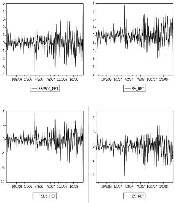
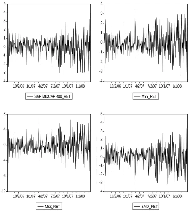
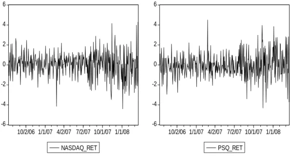
Figure 1-4 show the graphs for the daily returns of four U.S. stock market indices (Dow Jones Industrial Average Index, S&P500 Index, S&P400 MidCap Index, and Nasdaq100 index) as well as their corresponding Short/UltraShort ETFs and index futures spanning from 07/13/2006 to 03/18/2008. The returns of all stock market indices, ETFs, and index futures are defined as rt =100(log(ptclose/ptclose−1 )). As we can see, the shape of figure of stock index and index futures are very similar, and so are the Short and UltraShort ETF. Also, the returns of Short (UltraShort) ETFs are (twice) opposite to those of their benchmark. This reveals the nature of Short and UltraShort ETFs.
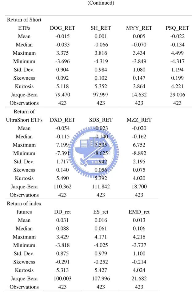
The descriptive statistics for the returns of these univariate series spinning from 07/13/2006 to 03/18/2008 are given in Table 2. The table shows that the mean returns of the four U.S. stock indices and their index futures are positive, and those of the short ETFs are all negative. This result is agreeing with the feature of short ETFs. The mean returns of Short/UltraShort ETFs are not exactly the value that inverse and twice the inverse of mean returns of their benchmarks, while the mean returns of index futures are very close to the returns of their corresponding U.S. stock indices. The standard deviations in this table also reveal that the Nasdaq100 index and its ETF product are more volatile than other indices and their ETF products. Besides, the standard deviations of Short ETFs and index futures are close to those of their benchmarks whereas the standard deviations of UltraShort ETFs are close to twice the values of their benchmarks. As for the higher moments of the return data, each of them has the excess kurtosis. This indicates that these data exhibit fat-tail distributions. Furthermore, return data of the four stock indices and their related index futures have negative skewness while return data of each short ETF has positive skewness. As to all the data series, the Jarque-Bera statistics strongly reject the null hypothesis of a normal distribution.
4.3 Empirical Analysis
< Table 3 is inserted about here > < Table 4 is inserted about here > < Table 5 is inserted about here > < Table 6 is inserted about here >
Table 3-6 present the empirical results of the estimation with the DCC model over the sample period from 07/13/2006 to 03/18/2008. Because of the procedure for parameters which are
estimated under the setting of standard DCC mode, we divide these tables into two parts consistent with the two steps in the DCC estimation. In Panel A of each table, we apply the GARCH model to individual assets to obtain the standardized residuals. Then, these standardized residuals series are brought into the second stage for dynamic conditional correlation estimating, and we show the estimated parameters of DCC model in Panel B of each table.
Furthermore, in panel A of Table 3-6, we can find that most of the coefficients estimated in the univariate GARCH (1,1) models are significant under 5% level excluding some coefficients of constant parameters in the conditional variance equations. The results reveal that very strong time-varying conditional heteroskedasticity is shown by the large t-statistics of the coefficients of the lagged squared residuals (α) and the lagged conditional variance terms (β). Besides, the sums of α+β for all series are near to one, and this is the evidence that there exists strong persistence in the conditional variances.
Finally, in Panel B of Table 3-6, the results show that almost all of the estimated coefficients (b) are significant at 5% level. These outcomes indicate that the correlations are significantly dynamic, and we can conclude that current dynamic conditional correlations are significantly affected by previous dynamic conditional correlations.
Based on the results above, we will focus on the tracking errors of each ETF in this section. First, the comparison of the tracking error between Short ETF and UltraShort ETF related to the same benchmark will be delivered. Furthermore, we try to observe whether the less perfect conditional correlation leads to the larger tracking error. Although the conditional correlations between returns of stock market indices and returns of their short ETF products are negative, we modify these numbers to positive for intuitive understanding. Then, we will also make the comparison of tracking error across the different stock market indices. Besides,
we will investigate the relationship between tracking error and trading volume of each short ETF as well as the relationship between tracking error of ETF and the return volatilities of its corresponding index futures.
< Table 7 is inserted about here > < Table 8 is inserted about here >
Table 7 show that all of the coefficients estimated in the univariate GARCH (1,1) models are significant under 5% level. The results reveal very strong time-varying conditional heteroskedasticity. The sums of α+β for are near to one, and this is the evidence that there exists strong persistence in the conditional variances. Table 8 presents the descriptive statistics of the tracking error (TE) between the Dow Jones Industrial Average index (DJIA) and its corresponding ETFs. As we can see, the TE also presents the fat-tail distributions and is found to reject the null hypothesis of a normal distribution. This indicates that the TE also has the same characteristics like most of the financial data. Also, in Table 8, the mean of TE between DJIA and its related Short ETF (DOG) is smaller than that between DJIA and UltraShort product (DXD). This means, on average, the DXD has the larger TE than that of DOG while the standard deviation between DOG and DXD does not have large differences. Based on these results, a conclusion can be made that the TE of DOG is smaller than TE of DXD.
< Figure 5 is inserted about here >
Figure 5 shows the comparison between the dynamic conditional correlation and the tracking error of short ETFs related to the DJIA. Although we can’t observe the perfect relationship between these two series, the less perfect conditional correlation seems to produce the larger tracking error. This phenomenon exists in both DOG and DXD. The
unconditional correlation between the TE and the dynamic conditional correlation for DOG is -0.557 while that for DXD is -0.377, which is much lower.
< Table 9 is inserted about here > < Table 10 is inserted about here >
Table 9 reveals that all of the coefficients estimated in the univariate GARCH (1,1) models are significant under 5% level except one coefficients of constant parameter. Table 10 shows the descriptive statistics of the tracking error (TE) between the S&P500 index and its corresponding Short (SH)/UltraShort (SDS) EFTs. The TE series of the SH presents the fat-tail distributions, whereas that of SDS is not. Both series are found to reject the null hypothesis of a normal distribution. Moreover, as shown in Table 10, both the mean and the standard deviation of TE between S&P500 and its related UltraShort ETF (SDS) outperform that between S&P500 and its Short product (SH). As a result, we can conclude that the SDS is better on the tracking ability than SH.
< Figure 6 is inserted about here >
Figure 6 shows the comparison between the dynamic conditional correlation and the tracking error of short ETFs related to the S&P500. In this figure, the relationship between these two series is not obvious. However, we still find the positive unconditional correlations between these two series. The value for SH is -0.529, and the value is only -0.112. Consequently, the less perfect conditional correlation will cause the TE to be larger.
< Table 11 is inserted about here > < Table 12 is inserted about here >
Table 11 reveals that all of the coefficients estimated in the univariate GARCH (1,1) models are significant under 5% level. Table 12 shows the descriptive statistics of the tracking error (TE) between the S&P400 MidCap index and its corresponding Short (MYY)/UltraShort (MZZ) EFTs. The TE series of the MYY and MZZ present the fat-tail distributions, and both series are found to reject the null hypothesis of a normal distribution. Furthermore, Table 12 also exhibit that both the mean and the standard deviation of TE between S&P400 MidCap and its related Short ETF (MYY) outperform that between S&P400 MidCap and its UltraShort product (MZZ). Based on these results, we can conclude that the MYY is better on the tracking performance than MZZ.
< Figure 7 is inserted about here >
Figure 7 reveals the comparison between the dynamic conditional correlation and the tracking error of short ETFs related to the S&P400.MidCap. We can see the strong positive relationship between these two series. The unconditional correlation between these two series of Short ETF (MYY) is -0.726, and that of UltraShort (MZZ) is -0.598. The less perfect conditional correlation between S&P400 MidCap and its corresponding short ETFs also leads to larger TE for these two ETFs.
< Table 13 is inserted about here > < Table 14 is inserted about here >
Table 13 reveals that all of the coefficients estimated in the univariate GARCH (1,1) models are significant under 5% level. Table 14 shows the descriptive statistics of the tracking error (TE) between the NASDAQ100 index and its corresponding Short (PSQ) EFTs. The TE series of the PSQ shows the fat-tail distributions, and are found to reject the null hypothesis of a normal distribution. Furthermore, Table 12 exhibits the mean of TE is 0.317, and the
standard deviation is 0.247.
< Figure 8 is inserted about here >
Figure 8 reveals the comparison between the dynamic conditional correlation and the tracking error of PSQ. We can see the comovement between the two series is very obvious. The unconditional correlation between the two series of PSQ is -0.893.
After we investigate the TEs of each Short/UltraShort ETF related to the same stock market index, here we try to compare the TE of Short/UltraShort ETF related to the different stock market index. Specifically, we try to show which Short/UltraShort ETF, across the different stock market indices, has the smallest TE.
< Table 15 is inserted about here >
Table 15 shows the statistics of tracking error of Short/UltraShort ETFs across different market indices. As we can see in Table 15, the PSQ is the worst on tracking performance in the group of short ETFs because it has the largest mean and standard deviation of tracking error while in the group of UltraShort ETFs, the MZZ is the worst on tracking performance due to the same reason.
In this section, we will investigate the relationship between tracking error and trading volumes of each ETF.
< Figure 9 is inserted about here >
The relationsip between tracking error and trading volumes of the “Short”(DOG)/ “UltraShort”(DXD) ETF of Dow Jones Industrial Average index seems vague. The unconditional correlation of these two series is 0.538 for DOG and 0.621 for DXD. This result shows that the larger the volumes, the larger the tracking error.
< Figure 10 is inserted about here >
In figure 10, we can’t not see clearly the relatioship between tracking error and trading volumes of the “Short”(SH)/ “UltraShort”(SDS) ETF of S&P500. We report that the unconditional correlation of these two series is 0.526 for SH and 0.857 for SDS. This result also shows that the larger the volumes, the larger the tracking error.
< Figure 11 is inserted about here >
In figure 11, the relatioship between tracking error and trading volumes of the “UltraShort”(MZZ) ETF is easier to observe than that of “UltraShort”(MZZ) ETF . The unconditional correlation of these two series is 0.439 for MZZ, and the value is mush smaller for MYY (0.007). This result reveals that the larger the volumes, the larger the tracking error.
< Figure 12 is inserted about here >
In figure 12, it’s hard for us to tell whether there is any relation between tracking error and trading volumes of the “Short”(PSQ) ETF. The unconditional correlation of these two series is only 0.191. This result also reveals that there is weak positive relation between the tracking error and trading volumes.
< Table 16 is inserted about here >
We utilize Table 16 to discuss the positive relationship between tracking error and trading volumes of each ETF. As we can see in Table 16, the higher correlation between tracking errors and trading volumes accompanies higher trading volumes. One possible reason for this phenomenon is that when the trading volumes go too large, the large trading volumes themselves generate the large tracking errors. This implies that when investors throng to market to buy these products, the over-trading will produce tracking errors. We can see the trading volumes of MYY and MZZ.
When the trading volumes are six times more for MZZ than MYY, the unconditional correlation goes from 0.007 for MYY to o.439 for MZZ
< Table 17 is inserted about here >
We use Table 17 to confirm our conjecture. In Table 17, we can find that the more the trading volumes, the bigger the tracking errors of each short ETF except MYY. This table also shows that the tracking errors come from the quarter which contains the larger trading volumes, are larger than the average tracking errors. Because of this reason, we conclude that the over-trading will lead to larger tracking error.
We will investigate the relationship between tracking error and volatilities of index futures in this section. ProShares uses index futures to rebalance its UltraShort ETFs daily to keep leverage consistent with each ETF’s daily investment objective so ProShares uses more index futures on UltraShort ETFs than on Short ETFs. When the volatilities of index futures go up, it may cause ProShares to miss the target prices and lead to tracking errors of ETFs. Because of this reason, we presume that volatilities of index futures have more influences on tracking errors of the UltraShort ETF than on those of Short ETF.
< Table 18 is inserted about here >
Table 18 reveals that all of the coefficients estimated in the univariate GARCH (1,1) models are significant under 5% level except one coefficients of constant parameter. The results show very strong time-varying conditional heteroskedasticity. The sums of α+β for are near to one, and this is the evidence that there exists strong persistence in the conditional variances.
After the the estimations of GARCH (1,1) for each index futures are made, we can difine the conditional standard deviations form GARCH (1,1) as the volatilities of index futures. Now we can use these results to discuss the relationship between the volatilities of index
futures and the tracking errors.
< Figure 13 is inserted about here >
Figure 13 shows that the relationsip between the tracking error of DOG/DXD and the volatilities of DJIA index futures seems to correlate positively. The unconditional correlation of these two series is 0.688 for DOG and 0.680 for DXD. This result shows that the tracking errors of “Short” (DOG)/”UltraShort” (DXD) ETF of DJIA are affected almost equally by the volatilities of DJIA index futures.
< Figure 14 is inserted about here >
The relationsip between the tracking error of SH/SDS and the volatilities of S&P500 index futures shown in Figure 14 also seems to correlate positively. The unconditional correlation of these two series is 0.676 for SH and 0.882 for SDS. This result shows that the volatilities of S&P500 index futures have more influences on the tracking errors of the UltraShort (SDS) ETF than on those of Short (SH) ETF.
< Figure 15 is inserted about here >
The relationsip between the tracking error of MYY/MZZ and the volatilities of S&P400 MidCap index futures shown in Figure 15 is obscure. The unconditional correlation of these two series is 0.388 for MYY and 0.556 for MZZ. This result shows that the volatilities of S&P400 MidCap index futures have more influences on tracking errors of the UltraShort (MZZ) ETF than on those of Short (MYY) ETF.
According to the daily holdings of short ETFs revealed by ProShares, this company uses more index futures on the UltreaShort ETFs than on the Short ETFs. Coinciding with this fact, our results show that the volatilities of S&P500 and S&P400 MidCap index futures have more influences on tracking errors of the UltraShort ETFs than on those of Short ETFs.
However, the tracking errors of “Short” (DOG)/”UltraShort” (DXD) ETF of DJIA are affected almost equally by the volatilities of DJIA index futures.
Finally, the hedge performance of short ETFs will be shown, and the comparison will be made. Based on the results of performing DCC, we can use the conditional covariance and variance to calculate the hedge ratios.
< Figure 16 is inserted about here > < Figure 17 is inserted about here >
Figures 16 and 17 show that the minimum-variance hedge ratios (MVHRs) for stock market indices using their related Short ETF are all close to 1 and the values are close to 0.5 using their related UltraShort ETF. We can conclude that the basic functions of the Short ETF and the UltraShort ETF exist.
< Table 19 is inserted about here >
Table 19 reports that there is no certain answer that which knid of ETF outperform the other kind when it comes to hedging performance. For ETFs relate to DJIA, the Short (DOG) ETF has the better hedging performance than the UltraShort (DXD) ETF. The Short ETF (MYY) of S&P400 MidCap also outperform MZZ in hedging performance while the UltraShort (SDS) ETF of S&P500 outperform SH in hedging performance. Futhermore, for the comparison across different market indices, the MYY has the best hedging performance among the Short ETFs. SDS has the best hedging effectiveness among the UltraShort ETFs.
Ⅴ. Conclusion
We investigate the tracking errors and the hedging effectiveness of each short ETF. This article shows that when it comes to tracking errors of Short/UltraShort ETFs related to the same benchmark, the Short ETFs of DJIA and S&P400 MidCap outperform the UltraShort ETFs of these two indices. On the contrary, the UltraShort ETF of S&P500 has the better tracking ability than the Short ETF of the S&P500. As for the cross indices comparison, the Short ETF of NASDAQ100 is the worst on tracking performance in the group of Short ETFs while the MZZ has the worst tracking ability in the group of UltraShort ETFs. Still, after the time-varying correlations between ETFs and their benchmark are estimated from the DCC model, we report the negtive unconditional correlation between tracking errors and these time-varying correlations. This result corroborates that the unperfect correlation between ETFs and their benchmarks will lead to tracking errors as mentioned by Hehn (2005).
Furthermore, we also examine the relationship between tracking errors and volatilities of their related index futures as well as that between tracking errors and trading volumes. We conclude that the tracking errors of DOG and DXD are affected almost equally by the volatilities of DJIA index futures while the volatilities of S&P500 (S&P400 MidCap) index futures have more influences on tracking errors of SDS (MZZ) than on those of SH (MYY). The results, except for the short ETFs of DJIA, coincide with the facts that ProShares uses more index futures on UltraShort ETFs than on Short ETFs. ProShares uses index futures to rebalance its UltraShort ETFs daily to keep leverage consistent with each ETF’s daily investment objective. When the volatilities of index futures go up, it may cause ProShares to miss the target prices and lead to tracking errors of ETFs. We also find that over-trading on the shot ETFs may lead to larger tracking errors, and this effect is quite obvious regarding MYY and MZZ.
ETFs outperform UltraShort ETF when DJIA and S&P400 MidCap are concerned while the UltraShort (SDS) ETF of S&P500 has the better hedging performance than SH. Besides, the MYY has the best hedging performance among the Short ETFs when SDS has the best hedging effectiveness among the UltraShort ETFs.