汽車音訊訊號處理系統之設計與實現

全文

(1)國立交通大學機械工程學系碩士論文. 汽車音訊訊號處理系統之設計與實現 Design and Implementation of Automotive Audio Signal Processing Systems. 研究生：洪志仁指導教授：白明憲教授中華民國九十七年七月.

(2) 汽車音訊訊號理系統之設計與實現 Design and Implementation of Automotive Audio Signal Processing Systems. 研究生：洪志仁指導教授：白明憲. Student：Jhih-Ren Hong Advisor：Mingsian R. Bai. 國立交通大學機械工程學系碩士論文. A Thesis Submitted to Institute of Mechanical Engineering College of Engineering National Chiao Tung University in partial Fulfillment of the Requirements for the Degree of Master in Mechanical Engineering July 2008 Hsinchu, Taiwan, Republic of China. 中華民國九十七年七月.

(3) 汽車音訊訊號處理系統之設計與實現. 學生：洪志仁. 指導教授：白明憲. 國立交通大學機械工程學系（研究所）碩士班. 摘. 要. 本論文研究重點在於應用在汽車上之立體空間音效處理系統的設計與實現。共提出十個演算法以克服不同乘客及輸入訊號數目的播放模式。其中，兩個分別針對雙聲道立體聲及 5.1 聲道輸入所設計的聲道擴展/縮減演算法，目的在於平衡車內前後側揚聲器之聲音輸出。而另外八個基於反算濾波的演算法則可分成兩大類，第一類方法根據在汽車內所量測之頭部相關轉移函數(HRTF)設計，此類方法考慮到因人體頭部、耳朵及軀幹所產生繞射及遮蔽效應。而第二類方法則稱為點接收器模型，用一個位於乘客頭部中心的點接收器來模擬聲音的傳播。所提出之演算法在不同的聆聽模式下，透過一系列包含車內定位實驗的主、客觀實驗加以比較。實驗結果透過多變異量分析(MANOVA)及費雪最小顯著差異法(Fisher’s LSD)的事後檢定(post hoc test)檢視是否有統計上的顯著差異。實驗結果指出，在單一乘客的情況下，反算濾波法表現較佳，而在多位乘客的情況下，聲道擴展/ 縮減法的表現優於其他處理方法。. i.

(4) Design and Implementation of Automotive Audio Signal Processing Systems. Student：Jhih-Ren Hong. Advisor：Dr. Mingsian R. Bai. Department (Institute) of Mechanical Engineering National Chiao Tung University. ABSTRACT. Design and implementation strategies of spatial sound processing are investigated in this paper for automotive scenarios.. Ten design algorithms are implemented for. various rendering modes with different number of passengers and input channels. Two up/downmixing algorithms aimed at balancing the front and rear reproduction are developed for the stereo two-channel input and the 5.1-channel input, respectively. Eight algorithms based on inverse filtering are implemented in two approaches.. The. first approach is based on binaural HRTFs (Head-Related Transfer Functions) measured in the car interior, which accounts for the diffraction and shadowing effect due to the head, ears and torso.. In the second approach termed the point-receiver. model, sound rendering is targeted at a point receiver positioned at the head center of the passenger. The proposed processing algorithms were compared via series of objective and subjective experiments under various listening conditions.. In. particular, a localization test was undertaken in the car interior to compare the proposed algorithms.. Test data were processed by the multivariate analysis of. variance (MANOVA) and the least significant difference method (Fisher’s LSD) as a post hoc test to justify the statistical significance. ii. The results indicate that inverse.

(5) filtering methods are preferred for the single passenger mode.. For the. multi-passenger mode, however, up/downmixing algorithms have attained better performance than the other processing techniques.. iii.

(6) 誌. 謝. 時光飛逝，兩年碩士班研究生涯轉眼就過去了。首先感謝指導教授白明憲博士的指導與教誨，使我順利完成學業與論文，在此致上最誠摯的謝意。而老師指導學生時豐富的專業知識，嚴謹的治學態度以及待人處事方面，亦是身為學生的我學習與景仰的典範。在論文寫作上，感謝陳宗麟和鄭泗東教授在百忙中撥冗閱讀並提出寶貴的意見，使得本文的內容更趨完善與充實，在此本人致上無限的感激。回顧這兩年的日子，承蒙同實驗室的博士班李志中學長、陳榮亮學長、林家鴻學長及碩士班陳暉文學長、莊崇源學長、楊鎮懇學長、郭軒愷學長、蕭博耀學長及張寰生學長在研究與學業上的適時指點，並有幸與同學黃兆民、謝秉儒及劉青育在學業上互相討論，在遭遇困挫時得以突破瓶頸。而與學弟艾學安、何克男、王俊仁、郭育志及劉冠良在生活上的朝夕相處，亦是值得回憶。沒有你們，我可能只能自己孤拎拎的去球場打球。最後僅將此篇論文，獻給我親愛的家人。感謝我的父親兼好友洪文憲先生總是給我無條件的支持與鼓勵，感謝已故的母親李娜珠女士從小對我無微不至的呵護與諄諄教誨；感謝女友孫銘儀總是陪在我身邊，聽我在得意時的自吹自擂，在我低潮時給我加油鼓勵。要感謝的人實在太多，上述名單如有疏漏，在此一併致上我最深的謝意。. iv.

(7) TABLE OF CONTENTS 摘. 要.............................................................................................................i. ABSTRACT...................................................................................................................ii. 誌. 謝.......................................................................................................iv. TABLE LIST..............................................................................................................vii FIGURE LIST.......................................................................................................... viii I.. INTRODUCTION ......................................................................................................1. II. UP/DOWNMIXING APPROACHES ............................................................................3 2.1. Up/Downmixing algorithms .................................................................................. 3. 2.2. Up/Downmixing approaches ................................................................................. 4. III. INVERSE FILTERING APPROACHES .......................................................................5 3.1. Multichannel inverse filtering............................................................................... 5. 3.2. System formulation ................................................................................................ 6. 3.2.1 HRTF model ............................................................................................................ 6 3.2.2 Point-receiver model ................................................................................................ 8 3.3. Equivalent complex smoothing techniques.......................................................... 9. 3.4. Inverse filtering-based approaches..................................................................... 10. 3.4.1 HRTF-based Inverse Filtering for single listener with upmixing (upmixingHIF1) method.................................................................................................................... 11 3.4.2 HRTF-based Inverse Filtering for single listener (HIF1) method.......................... 11 3.4.3 HRTF-based Inverse Filtering for two listener (HIF2) method ............................. 12 3.4.4 HRTF-based Inverse Filtering for two listener by filter superposition (HIF2a) method.................................................................................................................... 12 3.4.5 Point-receiver-based Inverse Filtering for single listener with upmixing (upmixingPIF1) method......................................................................................... 12 v.

(8) 3.4.6 Point-receiver-based Inverse Filtering for single listener (PIF1) method.............. 12 3.4.7 Point-receiver-based Inverse Filtering for two listener by filter superposition (PIF2a) method ...................................................................................................... 13 3.4.8 Point-receiver-based Inverse Filtering for four listener (PIF4) method................. 13. 4. OBJECTIVE AND SUBJECTIVE EVALUATIONS .....................................................13 4.1. Objective experiment........................................................................................... 14. 4.1.1 HRTF model .......................................................................................................... 14 4.2.2 Point-receiver model .............................................................................................. 15 4.2. Subjective experiment.......................................................................................... 16. 4.2.1 Experiment I........................................................................................................... 17 4.2.2 Experiment II ......................................................................................................... 19 4.2.3 Experiment III ........................................................................................................ 20 4.2.4 Experiment IV........................................................................................................ 21 4.3. 5. Localization test.................................................................................................... 21. CONCLUSIONS AND FUTURE WORK ....................................................................23. REFERENCES................................................................................................................26. vi.

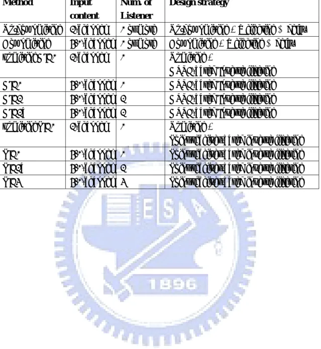
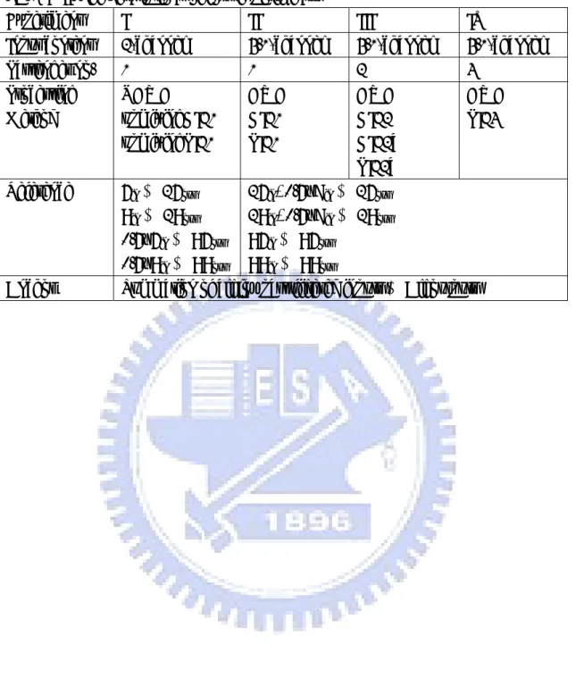
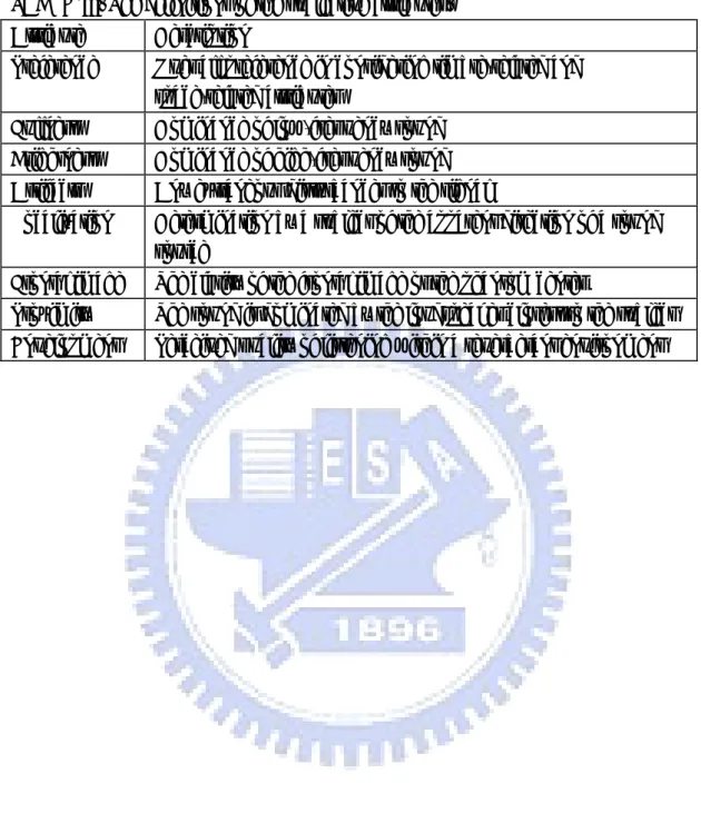
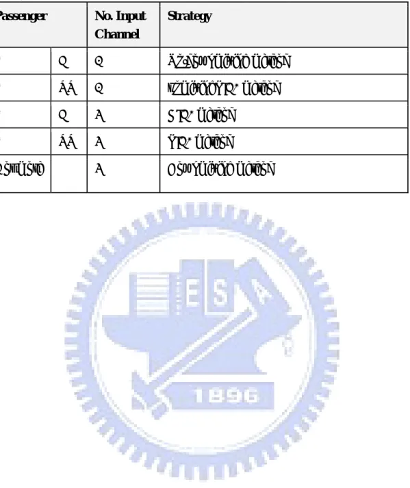
(9) TABLE LIST TABLE I. The descriptions of ten automotive virtual surround processing methods. 30 TABLE II. The descriptions of four experiments........................................................31 TABLE III. The definitions of the subjective attributes. .............................................32 TABLE IV. The description of five levels of grade for the localization test...............33 TABLE V. Summary of the strategies for various listening mode..............................34. vii.

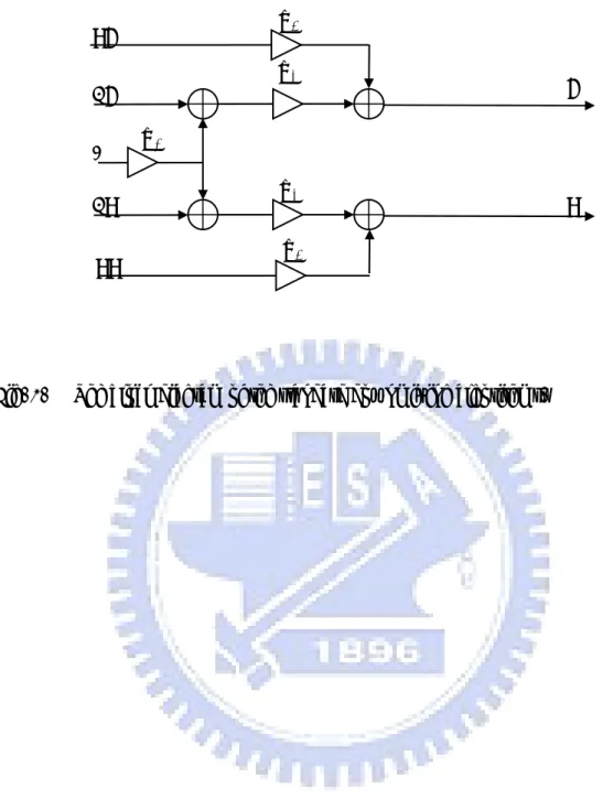
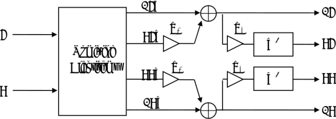
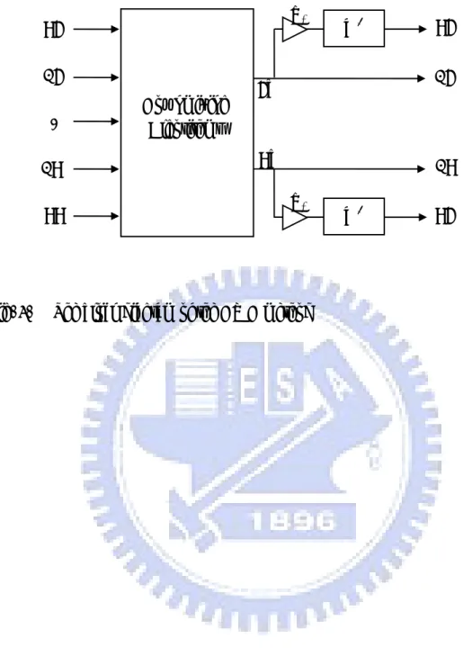
(10) FIGURE LIST Fig. 1.. The block diagram of the standard downmixing algorithms. ......................35. Fig. 2.. The block diagram of the reverberation-based upmixing algorithms. (a) The structure of the reverberator. (b) Block diagram of the upmixing algorithm ......................................................................................................................36. Fig. 3.. The block diagram of the UDWD method...................................................37. Fig. 4.. The block diagram of the DWD method......................................................38. Fig. 5.. The block diagram of the multichannel model matching problem. L: number of control points, M: number of loudspeakers, and N: number of program input. ............................................................................................................39. Fig. 6.. The geometry of HRTF model.....................................................................40. Fig. 7.. The geometry of point receiver model. The left plot shows the model for single listener case, and the right plot indicates the loudspeakers and the seats..............................................................................................................41. Fig. 8.. The geometry of the matching model for point receiver model in four-listener sitting mode.............................................................................42. Fig. 9.. The block diagram of the upmixingHIF1 method. ......................................43. Fig. 10. The block diagram of the HIF1 method, the HIF2 method and the HIF2a Method. ........................................................................................................44 Fig. 11.. The block diagram of the upmixingPIF1 method. ...................................45. Fig. 12.. The block diagram of the PIF1 method and the PIF2a method. ..............46. Fig. 13.. The block diagram of the PIF4 method. ..................................................47. viii.

(11) Fig. 14. The photos of the experimental arrangement (a) External view (b) Internal view..............................................................................................................48 Fig. 15. The frequency response of the HRTF-based acoustical plant at the front-left seat. (a) the front-side loudspeakers (b) the rear-side loudspeakers. The dotted lines represent the measured responses and the solid lines represent the smoothed responses................................................................................49 Fig. 16. The frequency responses of the HRTF-based inverse filters for front-left seat. (a) For the front sound image. (b) For the rear sound image...............50 Fig. 17. The frequency responses for the virtual sound image rendering.. The solid. lines represent the matching model responses M and the dotted lines represent the multichannel filter-plant product HC. (a) For the front sound image (b) For the rear sound image .............................................................51 Fig. 18. The frequency responses of the HRTF-based inverse filters for front-left and rear-right seats. (a) For the front sound image. (b) For the rear sound image 52 Fig. 19. The frequency responses for the virtual sound image rendering.. The solid. lines represent the matching model responses M and the dotted lines represent the multichannel filter-plant product HC. (a) For the front sound image (b) For the rear sound image .............................................................54 Fig. 20. The frequency responses of the point receiver-based acoustical plant at the front-left seat.. The dotted lines represent the measured responses and the. solid lines represent the smoothed responses...............................................55 Fig. 21. The frequency responses of the point receiver-based inverse filters for the front-left seat................................................................................................56. ix.

(12) Fig. 22. The frequency responses for the virtual sound image rendering.. The solid. lines represent the matching model responses M and the dotted lines represent the multichannel filter-plant product HC.....................................57 Fig. 23. The frequency responses of the point receiver-based acoustical plant for four listener mode.. The dotted lines represent the measured responses and. the solid lines represent the smoothed responses.........................................58 Fig. 24. The frequency responses of the point-receiver-based inverse filters for four-listener mode........................................................................................59 Fig. 25. The frequency responses for the virtual sound image rendering.. The solid. lines represent the matching model responses M and the dotted lines represent the multichannel filter-plant product HC.....................................60 Fig. 26. The means and spreads (with 95% confidence intervals) of the grades for Exp. I. (a) The first four attributes for FL seat (b) The last four attributes for FL seat (c) The first four attributes for RR seat (d) The last four attributes for RR seat. ..................................................................................................62 Fig. 27. The means and spreads (with 95% confidence intervals) of the grades for Exp. II. (a) The first four attributes for FL seat (b) The last four attributes for FL seat (c) The first four attributes for RR seat (d) The last four attributes for RR seat. ..................................................................................64 Fig. 28. The means and spreads (with 95% confidence intervals) of the grades for Exp III. (a) The first four attributes (b) The last four attributes ..................65 Fig. 29. The means and spreads (with 95% confidence intervals) of the grades for Exp IV. (a) The first four attributes (b) The last four attributes ..................66. x.

(13) Fig. 30. The arrangement for localization test. The markers positioned on the boundary of the car at the eye level with resolution 30°. .............................67 Fig. 31. The results of the localization test. (a) Unprocessed case for FL seat. (b) Unprocessed case for RR seat.. (c) The downmixing method for FL seat.. (d) The downmixing method for RR seat. seat.. (f) The HIF1 method for RR seat.. (e) The HIF1 method for FL. (g) The PIF1 method for FL seat.. (h) The PIF1 method for RR seat. (i) The PIF4 method for FL seat. (j) The PIF4 method for RR seat. (k) The HIF2a method for FL seat. (l) The HIF2a method for RR seat....................................................................73 Fig. 32. The means and spreads (with 95% confidence intervals) of the grades for Exp. IV. (a) The first four attributes (b) The last four attributes. ................74. xi.

(14) I.. INTRODUCTION With the rapidly growing of the digital telecommunication and data storage. technologies, it is possible to have compelling listening experience in automobiles. In addition to the conventional audio systems such as the radio broadcast set and Compact Disc (CD) playback, the Digital Versatile Disc (DVD) playback is commonly equipping in the car nowadays so that the multi-channel audio content can be rendered in the automotive environments to bring about the quality audio reproduction. However, there remain numerous challenges in automotive audio reproduction due to the nature of automotive listening environment.. The confined space results in. much shorter reverberation times compared to those of a concert hall, and the proximity of windows and seats creates strong reflections [1]. The loudspeakers and seats are positioned in an asymmetric arrangement, and thus the loudspeakers lead to produce poor sound images. the reproduced sound.. Further, ambient noise decreases the dynamic range of. For these reasons, the interior of a car is known as a. notorious listening environment [2].. This motivates the current research to develop. automotive audio spatializers to create a proper listening environment for vehicles. In addition to conventional multi-channel panning techniques [3], there are two advanced methods for spatial audio rendering: binaural audio [4]–[17] and wave field synthesis (WFS) [18]–[21].. Binaural audio is usually intended for one user using a. pair of stereo loudspeakers.. This approach, however, suffers from the limited size. problem of the so-called “sweet spot” in which the system remains effective [12]–[17]. In the other extreme, the WFS technique is ideally immune from the sweet spot problem and the listeners are free to move in the reproduction area.. However,. considerable coverage of WFS in academia has not lead to widespread commercial adoption of this technique.. The key issue is that large number of loudspeakers, and 1.

(15) hence complex processing, is required in the use of this approach, which limits its implementation in practical systems.. Pragmatic approaches will be presented in this. study as a compromise between binaural audio and WFS. Although spatial audio reproduction has been studied extensively by researchers, little can be found for automotive applications with regards to this technology.. By. contrast, there are already some luxury cars in the market place which are equipped with multi-channel surround system.. These systems are usually comprised of many. high-quality loudspeakers alongside digital audio processors, e.g., Lexicon’s LOGIC 7™ [22], Dolby’s® Prologic II [23], and SRS® Labs’ SRS Automotive™ [24].. Logic 7. and Prologic II are upmixers for extending 2-5.1-channel systems.. Bose®. AudioPilot® [25], and Bang & Olufsen advanced sound system [26] can automatically adjust the volume according to the background noise.. Crockett et al. pointed out. new trends in automotive audio technology and suggested methods to improve stereo imaging for off-center listeners [27].. However, the majority of current commercial. automotive audio systems are based on panning or equalization methods.. For. instance, Pioneer’s® MCACC (Multi-Channel Acoustic Calibration) [28] compensates the acoustical plants between the listener’s position and each loudspeaker by a 9-band equalizer. Few of sophisticated and accurate approaches are employed to cope with the spatial sound rendering problem for automobile. In this paper, various inverse filtering and up/down mixing techniques are used to design the automotive audio spatializers. Ten strategies are proposed for various listener sitting modes and input channels. The proposed approaches have been implemented on a real car by using a fixed-point digital signal processor (DSP) and compared via series of objective and subjective experiments in accordance with various listening conditions. Furthermore, the localization tests are conducted to examine the source localization of the proposed approaches.. Test data were processed by multivariate analysis of variance 2.

(16) (MANOVA) [29] and least significant difference method (Fisher’s LSD) for post hoc test to justify the statistical significance.. II. UP/DOWNMIXING APPROACHES In this section, theories of the up/downmixing algorithms and design strategies based on up/downmixing algorithms are introduced.. For the situations that the. 2-channel input signals such as MP3, CD and radio broadcast are considered, the left-channel signals are fed to the front-left and the rear-left speakers in traditional automotive audio.. However, the problem of this approach is that the front and rear. channels are too correlated to create natural-sounding surround effect [2].. Thus,. referring to a previous subjective listening test, a reverberation-based upmixing algorithm that is found to be very effective in producing sense of space is employed for extending 2-channel input to 4-channel [30].. When upmixed signals or. 5.1-channel input content from Dolby Digital or DTS decoder in DVD players are available, it is improper to feed these signals directly to the rendering loudspeakers owing to the non-ideal loudspeaker/listener positions.. To cope with this problem,. concatenated upmixing and downmixing processing is required.. The standard. downmixing algorithm is employed in the up/downmixing-based methods to reduce the input channel from four to two with very low computational loading [31]. 2.1 Up/Downmixing algorithms First, the standard downmixing algorithm is introduced. The standard, ITU-R BS.775-1, describes in detail how to downmix multi-channel signals with simple gain adjustment [31]. algorithm.. Figure 1 shows the block diagram of the standard downmixing. The center channel is weighted by 0.71 (or -3 dB) and mixed into the. front channels.. Similarly, the rear left and the rear right surround channels are. weighted by 0.71 and mixed into the front left and the front right channels, 3.

(17) respectively. That is, L = FL + 0.71× C + 0.71× RL R = FR + 0.71× C + 0.71× RR. ’. (1). depending on the rendering loudspeaker system, the LFE channel can be mixed into the front channels as an option. Next, the reverberation-based upmixing algorithm is presented. diagram is illustrated in Fig. 2.. The block. In order to produce the ambience-enriched surround. channels, an artificial revereberator is employed.. The artificial reverberator is. composed of 3 parallel comb filters and a 3-layered nested-allpass filter as shown in Fig. 2(a).. In this paper, a space with medium room size is selected to be simulated. by the artificial reverberator. The parameters are tuned by the Genetic Algorithm (GA) [30].. The left and right input signals are summed as the input signal of the. reverberator. The difference between the left and right input signals is mixed into the reverberator output to enhance ambience.. The rear-left and rear-right channels. are weighted and made 180° out of phase. 2.2 Up/Downmixing approaches For two-channel input, the Up/Downmixing with Weighting and Delay (UDWD) method is developed to improve the spaciousness and balance the front and rear. Figure 3 shows the block diagram, in which the input signals are first extended to four-channel by a reverberation-based upmixer and then downmixed into two-channel. The processed two-channel signals are next fed to the front and rear channels with delay (20ms) and weightings (0.65). For 5.1-channel input, the Downmixing with Weighting and Delay (DWD) method is developed for inputs in 5.1-format, as depicted in the block diagram of Fig. 4. In the method, the center channel is first mixed into the front two channels and then the ipsi-lateral channels are summed to produce the two frontal channels.. 4. Next,.

(18) the frontal channels are weighted and delayed to produce the rear channels. The remaining channel, LFE, is mixed into each loudspeaker, assuming that the subwoofer is unavailable.. III. INVERSE FILTERING APPROACHES Design procedure of multichannel inverse filters and equivalent complex smoothing techniques are presented in this section. on inverse filtering are introduced.. Then, the design strategies based. The multichannel inverse filters serve two. purposes in this spatial audio problem. One is to ‘de-reverberate’ the room response and another is to position virtual sound images according to the standard 5.1-channel configuration [31].. In what follows, strategies based on two categories of acoustical. model will be discussed.. The first approach is based on the binaural HRTFs. (Head-Related Transfer Functions) which account for the diffraction and shadowing effect due to the head, ears and torso.. The second approach is the point-receiver. model which regards the passenger’s head as a simple point receiver at the center. Based on the HRTF model, four strategies are investigated to aim at reproducing four virtual sound images located at ±30° and ±110°, according to the International Telecommunications Union (ITU) standard, ITU-R Rec. BS.775-1. database measured by MIT Media Lab [32], [33] is employed.. The HRTF. Alternatively, four. strategies based on the point-receiver model are proposed to compensate the frequency response between the loudspeakers and the microphone placed at the point receivers. 3.1 Multichannel inverse filtering This inverse filtering problem can be viewed from a model-matching perspective, as shown in Fig. 5.. In the block diagram, x ( z ) is a vector of N. program inputs, v ( z ) is a vector of M loudspeaker inputs, and e ( z ) is a vector of 5.

(19) L error signals or control points.. M ( z ) is an L × N matrix of matching model,. H ( z ) is an L × M plant transfer matrix, and C ( z ) is a M × N matrix of the. inverse filters. The z − m term accounts for the modeling delay to ensure causality of the inverse filters.. For arbitrary inputs, minimization of the error output is. tantamount to the following optimization problem,. min M − HC C. 2. (2). F. where F symbolizes the Frobenius norm [34].. Using Tikhnov regularization, the. inverse filter matrix can be shown to be [35].. (. C = HH H + β I. ). −1. HH M. (3). The regularization parameter β can either be constant or frequency-dependent. In the paper, the criterion for choosing β is dependent on a gain threshold applied to C [11]. It is noted that the filter C in Eq. (3) is a frequency-domain formulation. Inverse Fast Fourier transform (FFT) along with circular shift (hence the modeling delay) are needed to obtain causal FIR filters.. 3.2 System formulation 3.2.1 HRTF model For single listener sitting on the arbitrary seat in the car, the geometry for the measurement is illustrated as Fig. 6. This system involves two control points for one listener’s ears, four loudspeakers, and four input channels.. Therefore, the 2×4. acoustical plant matrix H(z) and the 2×4 matching model matrix M(z) can be represented as: ⎡ H ( z ) H12 ( z ) H13 ( z ) H14 ( z ) ⎤ H ( z ) = ⎢ 11 ⎥ ⎣ H 21 ( z ) H 22 ( z ) H 23 ( z ) H 24 ( z ) ⎦. 6. (4).

(20) ⎡ HRTF30i M( z) = ⎢ c ⎣ HRTF30. HRTF30c. i HRTF110. HRTF30i. c HRTF110. c ⎤ HRTF110 , i ⎥ HRTF110 ⎦. (5). where the superscripts i and c refer to the ipsilateral and contralateral side, respectively. The subscripts 30 and 110 are the azimuths of the HRTF, respectively. This results in a 4×4 inverse filter matrix, however, the design of the inverse filter can be separated into two parts: the front and the rear. That is to say, the front-side loudspeakers are employed to generate the ±30° sound images, and the rear-side ones for ±110°.. Consequently, the plant, the matching model and the inverse filter. matrices can be represented as: ⎡ H ( z ) H12 ( z ) ⎤ R ⎡ H13 ( z ) H14 ( z ) ⎤ = z H F ( z ) = ⎢ 11 H , ( ) ⎢ H ( z) H ( z)⎥ ⎥ 24 ⎣ H 21 ( z ) H 22 ( z ) ⎦ ⎣ 23 ⎦. (6). ⎡ HRTF30i M F ( z) = ⎢ c ⎣ HRTF30. (7). i ⎡ HRTF110 HRTF30c ⎤ R z , ( ) M = ⎥ ⎢ c HRTF30i ⎦ ⎣ HRTF110. c ⎤ HRTF110 i ⎥ HRTF110 ⎦. ⎡C11F ( z ) C12F ( z ) ⎤ R ⎡ C11R ( z ) C12R ( z ) ⎤ C ( z) = ⎢ F ⎥ , C ( z) = ⎢ R ⎥, F R ⎣C21 ( z ) C22 ( z ) ⎦ ⎣C21 ( z ) C22 ( z ) ⎦ F. (8). where superscripts F and R denote the front-side and the rear-side, respectively. The inverse matrices can be obtained by Eq. (3). A great saving of computation can be obtained by applying this procedure. The number of the inverse filters reduces from sixteen (one 4×4 matrix) to eight (two 2×2 matrices). Next, two listeners sitting on different seats are concerned. In this problem, four control points for two listeners’ ears, four loudspeakers, and four input channels are involved. By following the step borrowed from single listener mode, the design of the inverse filter can be divided into two parts. Therefore, the acoustical plants are two 4×2 matrices, the matching models are two 4×2 matrices and the inverse filters are two 2×2 matrices:. 7.

(21) ⎡ H11 ( z ) H12 ( z ) ⎤ ⎡ H11 ( z ) H12 ( z ) ⎤ ⎢ H ( z) H ( z)⎥ ⎢ H ( z) H ( z)⎥ 21 22 22 F R ⎢ ⎥ ⎥ H ( z) = , H ( z ) = ⎢ 21 ⎢ H 31 ( z ) H 32 ( z ) ⎥ ⎢ H 31 ( z ) H 32 ( z ) ⎥ ⎢ ⎥ ⎢ ⎥ ⎣ H 41 ( z ) H 42 ( z ) ⎦ ⎣ H 41 ( z ) H 42 ( z ) ⎦. (9). ⎡ HRTF30i ⎢ HRTF30c F M ( z) = ⎢ ⎢ HRTF30i ⎢ c ⎢⎣ HRTF30. (10). i ⎡ HRTF110 HRTF30c ⎤ ⎥ ⎢ c HRTF30i ⎥ R ⎢ HRTF110 , ( ) M z = i ⎢ HRTF110 HRTF30c ⎥ ⎥ ⎢ c HRTF30i ⎥⎦ ⎢⎣ HRTF110. c ⎤ HRTF110 i ⎥ HRTF110 ⎥ c ⎥ HRTF110 i ⎥ HRTF110 ⎥⎦. ⎡C F ( z ) C12F ( z ) ⎤ R ⎡ C11R ( z ) C12R ( z ) ⎤ C F ( z ) = ⎢ 11F , C ( z ) = ⎥ ⎢ R ⎥ (11) F R ⎣C21 ( z ) C22 ( z ) ⎦ ⎣C21 ( z ) C22 ( z ) ⎦. 3.2.2 Point-receiver model In this section, two situations are considered. The first case is when single listener sitting on the arbitrary seat in the car, the geometry is illustrated as the left plot of Fig. 7. Based on this model, the acoustical plant matrix H(z) for single listener mode can be represented as four SISO (single-input-single-output) systems. Thus, Eq. (3) can be rewritten as. H m∗ ( z ) M ( z ) Cm ( z ) = H m∗ ( z ) H m ( z ) + β. (12). where the subscript m indicates the mth loudspeaker.. The frequency response. function measured in an anechoic chamber is designated as the matching model M(z), where the loudspeaker used in matching model measurement is the same type of the one in a realistic car. Therefore, four SISO inverse filters C(z) are obtained. The second case is when four listeners sitting on the front-left, front-right, rear-left and rear-right seats, respectively. This issue involved four control points for four listeners, four loudspeakers and four input channels.. For convenience, the. transfer function between the mth (m=1~4) control point and nth (n=1~4) loudspeaker is expressed as H mn ( z ) . The geometry for representation of the positions of four control points and four loudspeakers are shown in the right plot of Fig. 7. Therefore, 8.

(22) H(z) can be formulated as ⎡ H11 ⎢H H ( z ) = ⎢ 21 ⎢ H 31 ⎢ ⎣ H 41. H12. H13. H 22. H 23. H 32 H 42. H 33 H 43. H14 ⎤ H 24 ⎥⎥ H 34 ⎥ ⎥ H 44 ⎦. (13). Furthermore, a free-field point source model is employed as the matching model. That is ⎡ e − jkal11 ⎢ ρ0 ⎢e − jkal21 M( z) = 4π ⎢ e − jka l31 ⎢ − jkal41 ⎢⎣e. / l11 e − jkal12 / l12 / l21 e − jka l22 / l22. e − jkal13 / l13 e − jkal23 / l23. e − jka l32 / l32. e − jkal33 / l33. / l41 e − jka l42 / l42. e − jkal43 / l43. / l31. e − jka l14 / l14 ⎤ ⎥ e− jkal24 / l24 ⎥ ω , ka = , − jka l34 c0 e / l34 ⎥ ⎥ − jka l44 e / l44 ⎥⎦. (14). where ka , ρ 0 and c0 denote the wave number, the density and the sound speed, respectively.. It is assumed that ρ 0 =1.21kg/m3 and c0 =343m/s.. The distance. between the nth source and the mth receiver is denoted as lmn . According to the arrangement shown in Fig. 8, the distance lmn can be calculated. Finally, the 4×4 inverse filters matrix is derived from the aforementioned procedures.. 3.3 Equivalent complex smoothing techniques It is impractical and not robust to implement the inverse filters based on the measured room response due to its highly complex dynamics and measurement errors associated with it [36]. Some pre-processing should be applied prior to the design of the inverse filters.. A simple but elegant way is to smooth the peaks and dips of the. acoustic plant using the generalized complex smoothing technique suggested by Hatziantoniou and Mourjopoulos [37]. There are two methods for implementing complex smoothing.. The first method, uniform smoothing, is to calculate the. impulse response using the inverse FFT of the frequency response. Then, apply a time-domain window to truncate and taper the impulse response, which in effect smoothes out the frequency response. Finally, calculate the ‘smoothed’ frequency 9.

(23) response by FFT of the modified impulse response. Alternatively, a nonuniform smoothing method can also be used. This method performs smoothing directly in the frequency domain.. The frequency response is circularly convolved with a. frequency-dependent window whose bandwidth increases with frequency.. This. method is based on the notion in psychoacoustics that the spectral resolution of human hearing increases with frequency. The expression of nonuniformly smoothed frequency response is given as [37]. H ecs ( k ) = H cs ( k ) H cs ( k ) =. k +m(k ). ∑. i=k −m(k ). H ts ( k ) =. H ts ( k ). (15). H cs ( k ). H R ( k )Wsm ( i − k + m ( k ) ) + j. k +m( k ). ∑. i=k −m( k ). k +m(k ). ∑. i =k −m(k ). {⎡⎣ H. R. ( k )⎤⎦. 2. H I ( k )Wsm ( i − k + m ( k ) ) (16). }. + ⎡⎣ H I ( k ) ⎤⎦ Wsm ( i − k + m ( k ) ) , 2. (17). where k, 0 ≦ k ≦ J−1, is the frequency index and m(k) is the smoothing index corresponding to the length of the smoothing window.. The smoothing window. Wsm(i) is given by ⎧ 1 i=0 , ⎪ ⎪ 2b ( m ( k ) + 1) − 1 ⎪ ⎪ b − ( b − 1) cos ⎡⎣(π m ( k ) ) ( k − J ) ⎤⎦ Wsm ( i ) = ⎨ , i = 1,..., m ( k ) 2b ( m ( k ) + 1) − 1 ⎪ ⎪ ⎪ b − ( b − 1) cos ⎡⎣(π m ( k ) ) k ⎤⎦ i = m ( k ) + 1,..., 2m ( k ) , ⎪ 2b ( m ( k ) + 1) − 1 ⎩. (18). The integer m(k) can be considered as a bandwidth function by which a fractional octave or any other nonuniform frequency smoothing scheme can be implemented. The variable b determines the roll-off rate of the smoothing window. case when b = 1, the window reduces to a rectangular window.. 3.4 Inverse filtering-based approaches 10. As a special.

(24) 3.4.1 HRTF-based. Inverse. Filtering. for. single. listener. with. upmixing. (upmixingHIF1) method The upmixingHIF1 method is developed to deal with the single listener mode with two-channel input contents. The block diagram of the upmixingHIF1 method is shown in Fig. 9, where two-channel input signals are extended to four channels by the upmixing algorithm and next inverse filtered to produce the outputs.. For the design. of the inverse filters, the acoustical plants H(z) are the frequency response functions between the input to the loudspeaker and the output to the microphone mounted in KEMAR’s (Knowles Electronics Manikin for Acoustic Research) [32] ears, as formulated in Eq. (6). The matching model matrices and the calculated inverse filters were presented as Eqs. (7) and (8).. In addition, some listeners reported that. the sound image width is slightly compromised in applying inverse filtering in an informal listening test. To reconcile the problem, the weighted (0.45) and delayed (4 ms) four-channel inputs are mixed into the respective channels. It is noted that this processing will also be applied in all the inverse-filtering-based methods.. 3.4.2 HRTF-based Inverse Filtering for single listener (HIF1) method The structure of the HIF1 method shown in the block diagram of Fig 10 is the same as that of the upmixingHIF1 method except that it does not require upmix processing. Given the 5.1-channel inputs and four loudspeakers, the center channel has to be attenuated before mixing into the front-left and front-right channels. Next, front two channels and rear two channels are fed to the respective inverse filters. The remaining channel, LFE, is mixed into each loudspeaker, assuming that the subwoofer is unavailable. It is note that the inverse filters used in the HIF1 method are the same with the upmixingHIF1 method.. 11.

(25) 3.4.3 HRTF-based Inverse Filtering for two listener (HIF2) method The HIF2 method aims at the two listener mode with 5.1-channel inputs. The system formulations are shown in Eqs. (9) to (11). Since the inverse filters are two 2×2 matrices, the block diagram is the same as the HIF1 method, even though the design of the inverse filters is quite different from the HIF method.. 3.4.4 HRTF-based Inverse Filtering for two listener by filter superposition (HIF2a) method Like the function of the HIF2 method, the HIF2a method is developed to cope with two-listener mode with 5.1-channel input. Due to the linearity of acoustics, the design procedures of the HIF2a method can be separated into two steps. The first step is to design the inverse filters for each listener.. Next step, by adding the. calculated filter coefficients, two 2×2 inverse filter matrices can be obtained.. 3.4.5 Point-receiver-based Inverse Filtering for single listener with upmixing (upmixingPIF1) method The upmixingPIF1 method is a point-receiver-based inverse filtering method exploited for the scenario of single listener with two-channel inputs. This method is based on the concepts of the Pioneer’s® MCACC [28] system but it is more accurate in frequency resolution since the FIR inverse filter is employed to compensate the acoustical plants instead of the simple equalization. The problem can be formulated as four SISO systems so that the four inverse filters can be obtained by Eq. (12). The block diagram is shown in Fig. 11, in which the input signals are extended to four-channel and next fed to respective inverse filters.. 3.4.6 Point-receiver-based Inverse Filtering for single listener (PIF1) method 12.

(26) Besides the upmixing processing, the scheme of the PIF1 method is the same as that of the upmixingPIF1 method since this approach is intended for the 5.1-channel input. As presented in Fig. 12, the center channel has to be weighted before mixing into the front-left and front-right channels. The front two channels and rear two channels are then fed to the respective inverse filters.. 3.4.7 Point-receiver-based Inverse Filtering for two listener by filter superposition (PIF2a) method The PIF2a method is a solution to the problem of the two listener mode with 5.1-channel input, also. Figure 12 shows the block diagram. Similar to the concept of the HIF2a method, the inverse filter is obtained by adding the filter coefficients designed for each control point. Thus, the structure of this method is in common with the PIF1 method.. 3.4.8 Point-receiver-based Inverse Filtering for four listener (PIF4) method Except the single and the two-listener modes, the PIF4 method is devised for four listener mode with 5.1-channel input. As mentioned in Eq. (13) and (14), the acoustical plant and matching model are both 4×4 matrices. Therefore, the 4×4 inverse filter matrix can be obtained by Eq. (3). Fig. 13 shows the block diagrams of the PIF4 method. The center channel is mixed into the front channels and next the front and rear-channel signals are filtered directly.. 4 OBJECTIVE AND SUBJECTIVE EVALUATIONS A series of objective and subjective experiments were undertaken to evaluate the performance of the methods mentioned above.. Ten processing approaches are. summarized in Table I. These experiments were conducted in a Opel Vectra 2-liter 13.

(27) sedan equipped with a DVD player, a 7-inch LCD display, a multichannel audio decoder, and four loudspeakers (two mounted in the lower panel of the front door and two behind the backseat), as shown in Fig. 14(a). The experimental arrangement inside the car is shown in Fig. 14(b). A fixed-point digital signal processor (DSP), Blackfin-533, of Analog Device semi-conductor is employed to implement the algorithms. The microphone GRAS 40AC and the preamplifier GRAS 26AC were used for measuring acoustical plants.. 4.1 Objective experiment 4.1.1. HRTF model In this section, strategies based on the HRTF model are evaluated, including the. upmixingHIF method, the HIF method, the HIF2 method and the HIF2a method. For the case when single passenger sitting on FL (front-lest) seat is considered, the plants can be represented as Fig. 6 and formulated as Eq. (6).. Figures 15(a) and (b). show the frequency responses of front-side and rear-side plants, respectively. The upper-left, upper-right, lower-left and lower-right plots in Fig. 15(a) signify the H11F , H12F , H 21F and H 22F , respectively.. The x-axis and the y-axis represent. frequency in Hz and magnitude in dB, respectively. The dotted lines and solid lines are the original measured responses and smoothed response, respectively. The spiky measured responses have been smoothed out effectively after applying the aforementioned equivalent complex smoothing technique. Comparison of the left column and the right column of Figs. 15(a) and (b) show that head shadowing is not significant due to boundary reflections in the small car cabin.. The frequency. responses of the inverse filters for the frontal and the rear acoustical plants are shown in Figs. 16(a) and (b), respectively. Figure 16(b) shows that the filter frequency responses above 6 kHz exhibit high gain because of the poor high-frequency response. 14.

(28) of the rear loudspeakers. In regularization of inverse filters, the gain is always restricted below 6 dB to prevent from overloading the filters.. The solid lines in Figs.. 17(a) and (b) represent 30° and 110° HRTF pairs, respectively, whereas the dotted lines represent the multichannel filter-plant product, H(ejω)C(ejω). The agreement between these two sets of responses is generally good below 6 kHz except that notable discrepancies can be observed, especially for the rear-loudspeaker case. The reason is that the inverse filters are gain-limited using regularization at the frequencies where the plants have significant roll-off. Next, the scenario of two listeners sitting on FL and RR seats simultaneously is examined. The proceeding design of inverse filers is suitable for the HIF2 method. The frequency responses of the inverse filters are illustrated in Figs. 18 (a) and (b), respectively.. Similar to the result for single listener, the frequency response of. inverse filters exhibit high gain in high frequencies.. Figures 19(a) and (b) show the. comparisons of the results for frontal and rear virtual sound image, respectively. Obviously, the performance of both the ipsilateral and contralateral responses can barely fit to the matching model response. The reason may be the non-square nature of inverse filter design (the acoustical plant H is a 4×2 matrix).. A further. comparison of the HIF2 and HIF2a methods will be presented in the following subjective evaluations. 4.2.2. Point-receiver model. In this section, strategies based on point receiver model are evaluated. At the first, situation when single listener sitting on FL seat is examined.. Under this. situation, the inverse filters employed in the upmixingPIF, PIF and PIF2a methods are designed. Figures 20(a) and (b) show the frequency responses between the four loudspeakers and the microphones placed at the center position of listener’s head (the control point). The upper and the lower rows of the figures are measured when the 15.

(29) front-side and rear-side loudspeakers are enabled, respectively. The left and right columns of the figures are measured when the left-side and right-side loudspeakers are enabled, respectively. For example, the upper-left plot is the frequency response measured between the control point and the front-left loudspeaker. The frequency responses of the inverse filters are shown in Fig. 21.. Similar to the results of the. HRTF model, the frequency response of the filters show high gain above 10 kHz due to the poor high-frequency response of rear loudspeakers.. In regularization of. inverse filters, the gain is always restricted below 9 dB to prevent from overloading the filters. Figure 22 represents the inverse filter-plant product, H(ejω)C(ejω). The agreement between these two sets of responses is generally good below 10 kHz except that notable discrepancies can be observed, especially for the rear-loudspeaker case. The second case, when four listener sitting on FL, FR, RL and RR seats, is considered. The frequency responses of the 4×4 plant matrix are shown in Fig. 23. It can be observed that only the most important features of the measured plant are remained.. Further, the frequency responses of the 4×4 inverse filter matrix are. illustrated as Fig. 24.. The gain is always restricted below 9 dB in regularization of. inverse filters to prevent from overloading the filters.. The inverse filter-plant. product is presented in Fig. 25. Below 7k Hz, these two sets of response seem to agree, however, notable discrepancies can be observed in high-frequency.. 4.2 Subjective experiment Ten automotive audio methods proposed in Sections II and III are compared via the following subjective listening experiments, according to a modified double-blind Multi-Stimulus test with Hidden Reference and a hidden Anchor (MUSHRA) [38]. The experiment cases are described in Table II.. In Experiment I, four songs in. two-channel PCM format involving various instruments with significant dynamic 16.

(30) variations were chosen to be the test materials.. In Experiments II to IV, four. 5.1-channel movies in Dolby Digital format were used. Both timbral and spatial qualities are considered. The loudness of each reproduced signal was adjusted to the same level by measuring the sound pressure level at each seat with a monitoring microphone. Eight subjective attributes employed in the tests, including preference, timbral attributes (fullness, brightness, artifact) and spatial attributes (localization, frontal. image, proximity, envelopment) are summarized in Table III. participated in each experiment.. Forty subjects. The subjects participating in the tests were. instructed with definitions of the subjective indices and the procedures before the listening tests. The subjects were asked to respond after listening in a questionnaire, with the aid of a set of subjective indices measured on an integer scale from −3 to 3. Positive, zero, and negative scores indicate perceptually improvement, no difference, and degradation, respectively, of the signals after processing with the audio spatializers.. The order of the attributes is randomized except that the index. preference is always the last question. On the average, it took approximately forty minutes to finish an experiment. In order to access statistical significance, the scores were further processed by using the MANOVA. If the significance level is below 0.05, the differences among all methods are considered statistically significant and then examined further by the Fisher’s LSD post-hoc test. 4.2.1. Experiment I. In this experiment, three methods for the listening positions at the FL and RR seats (representing the ‘extreme’ cases) and the two-channel input, including the UDWD method, the upmixingHIF1 method and upmixingPIF1 method are evaluated. Apart from these three methods, a hidden reference (H. R.) and an anchor (An.) are added into the comparison. The case in which two-channel stereo input signals are 17.

(31) fed to the respective front and rear loudspeakers is used as the hidden reference. The signal obtained by summing and lowpass filtering (with 4 kHz cutoff frequency) the two-channel input signals is used as the anchor that is also fed to all loudspeakers. Since the methods upmixingHIF1 and upmixingPIF1 are devised for single listener, this experiment is separated into two parts: the front-left seat and the rear-right seat. In FL position, the MANOVA output indicates that only the index artifact exhibited no significant difference among all methods in timbral quality (F = 1.08262,. p>0.367). However, in spatial quality, the indices localization (F = 1.8456, p > 0.154) and proximity (F = 2.57037, p>0.067) exhibited no significant difference among all methods.. Figures 26(a) and (b) show the means and spreads (with 95%. confidence intervals) of the grades of each subjective index. The x-axis and y-axis represent the method and grade, respectively. The results of Fisher LSD post hoc test indicted that the grades of the UDWD method and the upmixingPIF1 method are significantly higher than those of the hidden reference and the upmixingHIF1 method in preference and brightness.. In fullness, the grades of the inverse filter-based. approaches (upmixingHIF1 and upmixingPIF1) are significantly lower than those of hidden reference and the UDWD method. In the spatial attributes, the proposed approached are all significantly outperform the hidden reference in frontal and. envelopment, but there are no significant different among the methods in localization and proximity. In the RR position case, Figures 26(c) and (d) show the means and spreads (with 95% confidence intervals) of the grades of each subjective indices. The results of. post hoc test reveal that the grade of the upmixingPIF1 method is significantly higher than those of the other approaches in preference, notwithstanding the grades of the UDWD and the upmixingHIF1 methods are significant higher than the hidden reference. In brightness and fullness, result similar to the case of the FL position is 18.

(32) obtained. The proposed approaches receive lower grade in fullness, but higher grade in brightness.. In terms of artifact, the grade of the UDWD method is the highest. among all the approaches. This implies that no artifacts are audible during the UDWD processing. In localization, frontal and proximity, the proposed methods are all significant higher than the hidden reference; whereas only the UDWD and upmixingHIF1 methods perform significantly well to the reference. To summarize, the UDWD method and upmixingPIF1 method are the preferred choices for position FL and RR respectively, because of their rendering performance in preference and spatial quality. 4.2.2. Experiment II. The DWD, HIF1 and PIF1 methods and the unprocessed 5.1-channel reproduction are compared in this experiment. Because only four loudspeakers are available in this car, the center channel of the 5.1-channel input is attenuated by -3 dB and mixed into the frontal channels to serve as the hidden reference. In addition, the four-channel signals are summed and lowpass filtered (with 4 kHz cutoff frequency) is used as the anchor. Fifteen listeners participated in the test for the front left and rear right seats. Figures 27(a) and (b) show the means and spreads (with 95% confidence intervals) of the grades of all attributes for all methods for FL position, whereas Figs. 27(c) and (d) show those for RR position. For the FL position, the results of the post. hoc test indicate that the grades of the HIF1 method in preference and fullness are significantly higher than those of the DWD and the PIF1 methods.. In brightness,. only the grade of PIF1 methods is significantly higher than the hidden reference, and there is no significant different among the DWD method and the HIF1 method. Further, there is no significant difference among methods in the attribute artifact,. localization, proximity and envelopment. In frontal, the inverse filter-based methods 19.

(33) are significantly higher than the hidden reference and the DWD method. In the RR position, there is no significant difference among all the methods in. fullness, artifact and localization. However, the grades of the inverse filtering-based methods are significantly higher than those in others in preference and brightness. In addition, grades of all the proposed methods are significantly higher than the grade of the hidden reference but in frontal and proximity. Finally, only the HIF1 method significantly outperform to the hidden reference. In general, all grades received are higher for the rear seat than for the front seat. In particular, the HIF1 method received the highest grades in most attributes, especially in spatial attributes. A low computation complexity substitute would be the PIF1 method since it received the highest grade in many attributes as well. 4.2.3. Experiment III. Experiment III is intended for evaluating the methods designed for two-listener mode and 5.1-channel input.. Four methods are compared in this experiment,. including the DWD method, the HIF2 method, the HIF2a method and the PIF2a method. The hidden reference and the anchor cases are the same with those in experiment II.. Figures 28(a) and (b) show the means and spreads (with 95%. confidence intervals) of the grades of the first four and the last four attributes, respectively. The post hoc test reveals that there is no significant difference between the DWD method and HIF2a method, while the grades of both are significantly higher than the hidden reference in overall preference. In fullness and proximity, there is no significant difference among all proposed methods.. In brightness, result similar to. the experiment II is obtained, the inverse filtering-based methods receive significant higher grades than the hidden reference but there is no significant difference among these methods. The grade of artifact obtained using the HIF2 method is very low, implying that some artifacts are audible. 20. The reason might be the nature of.

(34) non-square inverse filter design.. In frontal and localization, the grades of all. proposed methods are significantly higher than the hidden reference. Finally, the HIF2a method performs best in envelopment among all methods. To conclude, the HIF2a method might be the best choice for spatial quality. It is noted that the result is contrary to our expectation that more inverse filters (HIF2) should mean better performance.. In terms of computation complexity and rendering performance, the. DWD method is the adequate approach for the two-passenger mode. 4.2.4. Experiment IV. In this experiment, methods developed for four-listener mode, including the DWD method and the PIF4 method, were compared. The hidden reference and the anchor cases are the same with those in experiment II.. The means and spreads (with. 95% confidence intervals) of the grades of the attributes are shown in Figs. 29(a) and (b). The results of MANOVA output indicate that there is no significant difference among the methods in the attributes artifact and envelopment.. Further, the results of. the post hoc test show that there is no significant difference between the DWD method and the PIF4 method in preference and proximity, but the grades of these two methods are all significantly higher than the hidden reference.. In the attributes. brightness, localization and frontal, the PIF4 method receives the significantly highest grade. Overall, the PIF4 method does not significantly outperform the DWD method in both timbral and spatial quality. Similar result can be obtained that the inverse filtering-based approaches do not outperform the DWD method in multi-listener mode.. 4.3 Localization test The foregoing subjective experiments were intended to compare the preference among different methods. In this section, a further examined subjective evaluation of source localization is carried out in a car. 21. Markers were positioned on the.

(35) boundary of the car at the eye level with resolution 30°, as shown in Fig. 30. Each stimulus was pink noise and consisted of a reference and a test signal. The reference signal is intended to present a virtual sound image at 0˚. However, some methods might not produce accurate center sound images. As the result, the subjects were asked to make the judgment in a questionnaire according to the test signal only. The reference and test signals had the same program inputs recorded at the format of Dolby AC3. Both the reference and test signals were 5 seconds long with a 3 seconds pause in between. Virtual sound image at 12 pre-specified directions with increment 30° azimuth are presented in the experiment. Listeners were trained by playing the stimuli prior to the experiments. Experiments were divided into two parts: listener sitting on FL seat and listener sitting on RR seat. The experiments were blind tests in that stimuli were played randomly without informing the subjects the source direction. Referring to the results of subjective listening experiment, five relatively well-performed strategies including the DWD method, the HIF1 method, the PIF1 method, the HIF2 method and the PIF4 method were compared in the localization test. Moreover, case of unprocessed signal is involved as a benchmark. The results of localization test are shown in Fig 31. The x-axis and the y-axis represent the target angle and the judged angle in degree, respectively. The size of each angle is proportional to the number of the subjects who localized the same perceived angle.. It is observed from the results that the performance of the HIF1. method do not agree with our expectation, notwithstanding it is good at producing the 0˚ sound image. On the other hand, the PIF1 method is found to be effective in localizing good frontal and rear sound images, albeit some front-back reversals. Contrary to our expectation, the DWD method has good performance in producing frontal sound images on FL position case.. Further, methods designed for. multi-listener mode (PIF4 and HIF2a) seemed to have difficulty localizing sources for 22.

(36) each position. To justify the finding, a MANOVA on the subjective localization result was conducted. The results were preprocessed into five levels of grade, as stated in Table IV. The MANOVA outputs indicate that there are significant differences among all methods, both on FL and RR seat. (F=21.296 for FL, F = 11.561 for RR) Figure 32 shows the means and spreads (with 95% confidence intervals) of the grades of these approaches. Next, the results of the post-hoc test show that there is no significant difference between the DWD method and the PIF1 method in FL position and the grades of these two methods are significantly higher than other methods and the unprocessed signals.. Notice that PIF4 method receives the lowest grade on FL. position. Further, there is no significant difference among the DWD method, the PIF1 method and the unprocessed case in RR position. Except these two methods, the grades of the other approaches are significantly lower than the unprocessed signal case. To conclude, the results of statistic analysis show that the DWD method and the PIF1 method perform well in source localization.. 5 CONCLUSIONS AND FUTURE WORK A comprehensive study has been conducted to explore various audio processing approaches for the automotive virtual surround audio systems via simulations and experiments. Ten processing methods have been presented. Two methods based on up/downmixing algorithms including the UDWD method and the DWD method are intended to improve the spaciousness and to balance the front and rear reproduction. These two methods are practical approaches in terms of computation complexity and audio performance. A reverberation-based upmixing algorithm is used to extend two-channel inputs to four-channel signals.. Further, a standard downmixing. algorithm is employed to convert 5.1-channel input to two-channel. Eight inverse filtering-based approaches are further divided into two groups: HRTF-based model 23.

(37) and point receiver-based model.. Four HRTF-based inverse filtering methods are. exploited to correct the car responses and then render a spatial listening environment. Four point-receiver-based inverse filtering methods intend to compensate the acoustical plants. It is summarized from the discoveries above that a simple design strategy can be formulated according to the number of passengers, using a hybrid approach, as presented in Table V. Conclusions can be drawn from the listening tests and the localization test as follows. First, for two-channel inputs, the UDWD method outperformed the upmixingHIF1 and upmixingPIF1 methods in the position FL. However, in the RR seat, the upmixingPIF1 method performed better than others. Second, for the single listener and 5.1-channel inputs, the HIF1 method received the highest grades in most attributes in the position FL, notwithstanding its poor performance in localization test. In addition, the HIF1 and PIF1 methods all receive high grade in many attributes at the rear-right seat.. Thus, referring to the. result of localization test, the PIF1 method would be the best choice. Third, for the two-listener mode, the HIF2a method receives high grade in most attributes, the strategy for multi-listener is chosen to be the DWD method. Since there are no significant difference between the DWD method and the HIF2a method, and grade of the DWD method is significantly higher than that of HIF2a methods in localization test. Similar conclusion can be drawn for the four-listener mode. Although the grades of the PIF4 method are slightly higher than those of the DWD method in most attributes, the poor performance in localization test and the high computational complexity lead to the PIF4 method becomes a less practical approach for producing spatial sound in the automobile.. It can be concluded that the inverse filtering did not. perform as well for the multi-listener mode as it did for the single passenger mode. The number of inverse filters increases drastically with number of passengers, rendering this scheme impractical in automotive applications. 24. Fourth, the.

(38) upmixingPIF1 method and the PIF1 method obtain low grades in both FL and RR seats.. Since these two methods are basically the same, except the upmixing. procedure due to different number of input.. The reason might be that the PIF. method produces an excessively narrow frontal sound image. Thus, it indicates that the spatial quality can be improved by incorporating a revereberator into the system. A number of topics are planned for future research. Increase the number of rending loudspeakers to devise strategies for luxury cars. Integration of present surround system to the other audio techniques such as equalizers, superbass systems, dynamic range control, Karaoke machines, acoustical echo and noise control, etc., should be investigated.. 25.

(39) REFERENCES [1] Y. Kahana, P. A. Nelson and S. Yoon, “Experiments on the synthesis of virtual acoustic sources in automotive interiors,” AES 16th international conference on spatial sound reproduction and applications, Paris, March 1999, 16-021. [2] M. R. Bai and C.C. Lee, “Comparative study of design and implementation strategies of automotive virtual surround audio systems,” J. Audio Eng. Soc. (submitted) [3] F. Rumsey, Spatial Audio (Focal Press, Oxford, Boston, 2001). [4] P. Damaske and V. Mellert, “A Procedure for Generating Directionally Accurate Sound Images in the Upper-half Space Using Two Loudspeakers,” Acoustica, vol. 22, pp. 154–162 (1969). [5] D. H. Cooper and J. L. Bauck, “Prospects for Transaural Recording,” J. Audio Eng.. Soc., vol. 37, pp. 3–19 (1989). [6] D. R. Begault, 3-D Sound for Virtual Reality and Multimedia (AP Professional, Cambridge, MA, 1994). [7] R. Schroeder and B. S. Atal, “Computer Simulation of Sound Transmission in Rooms,” IEEE International Convention, Record 7, pp. 150–155 (1963). [8] W. G. Gardner, “Transaural 3D Audio,” MIT Media Laboratory Tech. Report 342, (1995). [9] J. L. Bauck and D. H. Cooper, “Generalized Transaural Stereo and Applications,”. J. Audio Eng. Soc., vol. 44, pp. 683–705 (1996). [10] J. Blauert, Spatial Hearing: The Psychophysics of Human Sound Localization (MIT Press, Cambridge, MA, 1997). [11] M. R. Bai and C. C. Lee, “Development and Implementation of Cross-talk Cancellation System in Spatial Audio Reproduction Based on the Subband Filtering,” J. Sound Vib., vol. 290, pp. 1269–1289 (2006). 26.

(40) [12] W. G. Gardner, 3-D Audio Using Loudspeakers (Kluwer Academic, Boston, Mass, 1998). [13] D. B. Ward and G. W. Elko, “Effect of Loudspeaker Position on the Robustness of Acoustic Crosstalk Cancellation,” IEEE Signal Process. Lett., vol. 6, pp. 106–108 (1999). [14] T. Takeuchi and P. A. Nelson, “Robustness to Head Misalignment of Virtual Sound Imaging Systems,” J. Audio Eng. Soc., vol. 109, pp. 958–971 (2001). [15] T. Takeuchi and P. A. Nelson, “Optimal Source Distribution for Binaural Synthesis over Loudspeakers, J. Acoust. Soc. Am., vol. 112, pp. 2786–2797 (2002). [16] P. A. Nelson and J. F. W. Rose, “Errors in Two-point Sound Reproduction,” J.. Acoust. Soc. Am., vol. 118, pp. 193–204 (2005). [17] M. R. Bai, C. W. Tung, and C. C. Lee, “Optimal Design of Loudspeaker Arrays for Robust Cross-talk Cancellation Using the Taguchi Method and the Genetic Algorithm,” J. Acoust. Soc. Am., vol. 117, pp. 2802–2813 (2005). [18] P. A. Gauthier, A. Berry and W. Woszczyk, “Sound-field Reproduction In-room Using Optimal Control Techniques: Simulations in the Frequency Domain,” J.. Acoust. Soc. Am., vol. 117, pp. 662–678 (2005). [19] T. Betlehem and T. D. Abhayapala, “Theory and Design of Sound Filed Reproduction in Reverberant Rooms,” J. Acoust. Soc. Am., vol. 117, pp. 2100–2111 (2005). [20] G. Theile and H. Wittek, “Wave Field Synthesis: A Promising Spatial Audio Rendering Concept,” Acoust. Sci. and Tech., vol. 25, pp. 393–399 (2004). [21] S. Spors, A. Kuntz, and R. Rabenstein, “An Approach to Listening Room Compensation with Wave Field Synthesis,” AES 24th International conference on. multichannel audio, pp. 1–13, (AES, Canada, 2003). 27.

(41) [22] Lexicon, LOGIC 7™, http://www.lexicon.com/logic7/index.asp [23] Dolby®, Prologic II, http://www.dolby.com/professional/popup_PLII/ [24] SRS® Labs, SRS Automotive™, http://www.srslabs.com/ae-srsautomotivetech826.asp [25] Bose, AudioPilot®, http://www.bose.com/controller?event=VIEW_STATIC_PAGE_EVENT&url=/auto motive/innovations/audiopilot.jsp [26] Bang & Olufsen, Advanced sound system, http://www.bang-olufsen.com/page.asp?id=321 [27] B. Crockett, M. Smithers, and E. Benjamin, “Next Generation Automotive Research and Technologies,” AES 120th Convention (Paris, France, 2006). [28] Pioneer,. “MCACC. Multi-Channel. Acoustic. Calibration”,. http://www.pioneerelectronics.com/pna/article/0,,2076_4151_20157532,00.html# [29] S. Sharma, Applied Multivariate Techniques (John Wiley, New York, 1996). [30] M. R. Bai and G. Bai, “Optimal Design and Synthesis of Reverberators with a Fuzzy User Interface for Spatial Audio,” J. Audio. Eng. Soc., vol. 59, pp. 812–825 (2005). [31] ITU-R Rec. BS.775-1, “Multi-channel Stereophonic Sound System with or without Accompanying Picture,” International Telecommunications Union, Geneva, Switzerland (1992–1994). [32] W. G. Gardner and K. D. Martin, KEMAR HRTF measurements (MIT’s Media Lab, http://sound.media.mit.edu/KEMAR.html, 1994). [33] W. G. Gardner and K. D. Martin, “HRTF Measurements of a KEMAR,” J. Acoust.. Soc. Am., vol. 97, pp. 3907–3908 (1995). [34] B. Noble, Applied Linear Algebra (Prentice-Hall, 1988). [35] M. R. Bai and C. C. Lee, “Objective and Subjective of Effects of Listening 28.

(42) Angle on Crosstalk Cancellation in Spatial Sound Reproduction,” J. Acoust. Soc.. Am., vol. 120, pp. 1976–1989 (2006). [36] P. D. Hatziantoniou and J. N. Mourjopoulos, “Errors in Real-Time Room Acoustics Dereverberation,” J. Audio. Eng. Soc., vol. 52, pp. 883–899 (2004). [37] P. D. Hatziantoniou and J. N. Mourjopoulos, “Generalized Fractional-octave Smoothing of Audio and Acoustic Responses,” J. Audio. Eng. Soc., vol. 48, pp. 259–280 (2000). [38] ITU-R BS.1534-1, “Method for the Subjective Assessment of Intermediate Sound Quality (MUSHRA)”, International Telecommunications Union, Geneva, Switzerland (2001). [39] M. R. Bai, G. Y. Shih and C. C. Lee, “Comparative study of audio spatializer for dual-loudspeaker mobile phones,” J. Acoust. Soc. Am., vol. 121(1), pp. 298–309 (2007).. 29.

(43) TABLE I. The descriptions of ten automotive virtual surround processing methods.. Method. Input content. Up/downmixing 2-channel. Num. of Listener. Design strategy. 1 or more. Up/downmixing + Weighting & delay. Downmixing. 5.1-channel 1 or more. Downmixing + Weighting & delay. upmixingHIF1. 2-channel. 1. Upmixing + HRTF-based Inverse filtering. HIF1. 5.1-channel 1. HRTF-based Inverse filtering. HIF2. 5.1-channel 2. HRTF-based Inverse filtering. HIF2a. 5.1-channel 2. HRTF-based Inverse filtering. upmixingPIF1. 2-channel. 1. Upmixing + Point-receiver-based inverse filtering. PIF1. 5.1-channel 1. Point-receiver-based inverse filtering. PIF2a. 5.1-channel 2. Point-receiver-based inverse filtering. PIF4. 5.1-channel 4. Point-receiver-based inverse filtering. 30.

(44) TABLE II. The descriptions of four experiments. Experiment. I. II. III. IV. Input content. 2-channel. 5.1-channel. 5.1-channel. 5.1-channel. Passenger no.. 1. 1. 2. 4. Processing Method. UDWD upmixingHIF1 upmixingPIF1. DWD HIF1 PIF1. DWD HIF2 HIF2a PIF2a. DWD PIF4. Reference. Lin Æ FLout Rin Æ FRout 0.7×Lin Æ RLout 0.7×Rin Æ RRout. FLin+0.7×Cin Æ FLout FRin+0.7×Cin Æ FRout RLin Æ RLout RRin Æ RRout. Anchor. Summation of all lowpass filtered inputs Æ All outputs. 31.

(45) TABLE III. The definitions of the subjective attributes. Attribute. Description. Preference. Over all preference in considering timbre-related and space-related attributes. Fullness. Dominance of low-frequency sound. Brightness. Dominance of high-frequency sound. Artifacts. Any extraneous disturbances to the signal. Localization. Determination by a subject of the apparent direction of a sound source. Frontal image. The clarity of the frontal image or the phantom center. Proximity. The sound is dominated by the loudspeaker closest to the subject. Envelopment. Perceived quality of listening within a reverberant environment. 32.

(46) TABLE IV. The description of five levels of grade for the localization test. Grade. Description. 5. The perceived angle is the same as the presented angle. 4. 30˚ difference between the perceived angle and the presented angle. 3. Front-back reversal of the perceived angle identical to the presented angle. 2. 30˚ difference between front-back reversal of the perceived angle and the presented angle. 1. Otherwise. 33.

(47) TABLE V. Summary of the strategies for various listening mode. Passenger. No. Input Channel. Strategy. 1. FL. 2. Up/downmixing method. 1. RR. 2. upmixingPIF1 method. 1. FL. 4. HIF1 method. 1. RR. 4. PIF1 method. 4. Downmixing method. 2 or more. 34.

(48) w3. RL. w2. FL C FR RR. Fig. 1.. L. w1 w2. R. w3. The block diagram of the standard downmixing algorithms.. 35.

(49) -c3 -c2. z-M1. -c1 g1 z-N1. z-M2 g2. c1. z-M3. c2. z-N2. z-N3. c3 g3 (a). w1. L. FL w1. R. FR Reverb. w2. RL -1. RR w3. (b) Fig. 2.. The block diagram of the reverberation-based upmixing algorithms. (a) The structure of the reverberator. (b) Block diagram of the upmixing algorithm. 36.

(50) FL’ L. FL w1. RL’ Upmixing Algorithms. w1. RR’. w2. w2. z -D. RL. z -D. RR. R FR’. Fig. 3.. The block diagram of the UDWD method. 37. FR.

(51) w1. RL FL C FR. Downmixing Algorithms. R’. FR w1. The block diagram of the DWD method. 38. RL FL. L’. RR. Fig. 4.. z -D. z -D. RL.

(52) Modeling delay. Matching Model. z-m. M(z) L×N. Input signals x(z). Inverse filters. Plant. C(z). H(z). M×N. Fig. 5.. Speaker input signals L×M v(z). Desired signals d(z) Error e(z). Reproduced signals w(z). The block diagram of the multichannel model matching problem. L: number of control points, M: number of loudspeakers, and N: number of program input.. 39.

(53) H21. H12. H11. H22 H24 H14 H23. H13. Fig. 6.. The geometry of HRTF model.. 40.

(54) Loudspeaker 1 Loudspeaker 2. Loudspeaker 2 Loudspeaker 1. H1 H2. H3. Loudspeaker 3. Fig. 7.. 1. 2. 3. 4. H4. Loudspeaker 4. Loudspeaker 3. Loudspeaker 4. The geometry of point receiver model. The left plot shows the model for single listener case, and the right plot indicates the loudspeakers and the seats.. 41.

(55) Virtual source Receiver. 2. 1 2m 1. 2. 3. 4. 0.85m. 3. 4. 0.7m. Fig. 8.. The geometry of the matching model for point receiver model in four-listener sitting mode.. 42.

(56) w2 z -D FL. C11F C21F C12F FL’. C22F w2. L Upmixing Algorithms. FR’. w3 C11. RR’. z -D z -D. RL’. R. FR. R. RL. C21R C12R C22 w3. Fig. 9.. The block diagram of the upmixingHIF1 method.. 43. RR. R. z -D.

(57) w2 z -D FL. C. FL. C11F C21F. w1. C12F FR. C22F w2 w3. FR z -D z -D. C11R RL. RL. C21R. RR. C12R RR. C22R w3. z -D. Fig. 10. The block diagram of the HIF1 method, the HIF2 method and the HIF2a Method.. 44.

(58) w1 z -D FL. C1 FL. FR. C2. L Upmixing Algorithms. R. FR. z -D. w1 w2. RL RR. z -D RL. C3. RR. C4 w2. z -D. Fig. 11. The block diagram of the upmixingPIF1 method.. 45.

(59) w2. z -D. FL. FL. C1 w1. C FR. FR. C2 w2. z -D. w3 RL. z -D RL. C3. RR. RR. C4. w3. z -D. Fig. 12. The block diagram of the PIF1 method and the PIF2a method.. 46.

(60) FL C. C11. w1. FR. FL. C12. RL. C13. RR. C14 C21. FR. C22 C23 C24 C31. RL. C32 C33 C34 C41 C42 C43 C44 Fig. 13. The block diagram of the PIF4 method.. 47. RR.

(61) (a). DVD player. LCD. Front-right loudspeaker. (b) Fig. 14. The photos of the experimental arrangement (a) External view (b) Internal view.. 48.

(62) (a). (b) Fig. 15. The frequency response of the HRTF-based acoustical plant at the front-left seat. (a) the front-side loudspeakers (b) the rear-side loudspeakers. The dotted lines represent the measured responses and the solid lines represent the smoothed responses.. 49.

(63) (a). (b) Fig. 16. The frequency responses of the HRTF-based inverse filters for front-left seat. (a) For the front sound image. (b) For the rear sound image. 50.