國
立
交
通
大
學
資訊科學與工程研究所
碩
士
論
文
無 線 感 測 網 路 之 事 件 周 圍 查 詢 處 理 機 制
Event Surrounding Query Processing in
Wireless Sensor Networks
研 究 生:周佳欣
指導教授:彭文志 教授
無 線 感 測 網 路 之 事 件 周 圍 查 詢 處 理 機 制
Event Surrounding Query Processing in Wireless Sensor Networks
研 究 生:周佳欣 Student:Chia-Hsin Chou
指導教授:彭文志 Advisor:Wen-Chih Peng
國 立 交 通 大 學
資 訊 科 學 與 工 程 研 究 所
碩 士 論 文
A ThesisSubmitted to Institute of Computer Science and Engineering College of Computer Science
National Chiao Tung University in partial Fulfillment of the Requirements
for the Degree of Master
in
Computer Science
October 2007
Hsinchu, Taiwan, Republic of China
無線感測網路之事件周圍查詢處理機制
學生:周佳欣
指導教授
:彭文志
國立交通大學資訊科學與工程研究所碩士班
摘
要
在無線感測網路領域,事件的發生與偵測一直是很重要的ㄧ環。然而,事件
有可能在任何時間點演化,並且往任意方向蔓延,及早偵測並且提供即時的資訊
給使用者是非常重要的,使用者透過資訊的回報可以採取適當的動作,對事件發
展的情況取得控制。因此,在本篇論文我們提出ㄧ種新型態的空間查詢,簡稱為
『事件周圍查詢』,透過此查詢可以選出最靠近事件邊界的感測器節點來監控事
件,而被選出來的節點就稱之周圍節點。另外,我們為此提出兩個演算法,一個
是以 RNN 為基礎的演算法以及另一個 Greedy 演算法來處理事件周圍查詢。以
RNN 為基礎的演算法延伸現有的 RNN 查詢來選取周圍節點,然後找出它們之間
不能被感測到的漏洞,再選取適當的感測器節點去彌補此漏洞。Greedy 演算法每
次都去選取最靠近事件的感測器節點作為周圍節點,然後藉由鄰居關係的檢驗避
免選取多餘的感測器節點作為周圍節點。實驗結果顯示,Greedy 演算法在選取周
圍節點的數量跟所花的成本優於以 RNN 為基礎的演算法。
Event Surrounding Query Processing in Wireless Sensor Networks
Student:Chia-Hsin Chou
Advisors:Dr. Wen-Chih Peng
Institute of Computer Science
National Chiao Tung University
ABSTRACT
In many applications of wireless sensor networks, events evolve at anytime and in
any directions. Early detection and providing timely information are especially
im-portant for users to take events under control. In this paper, we propose a novel type
of spatial query, Event Surrounding query (abbreviated as ES query), in which sensor
nodes that are near to the boundary of events are selected for monitoring. Those nodes
selected by ES query are referred to as surrounding nodes. We propose two algorithms,
RNN-based algorithm and Greedy algorithm for event surrounding queries.
RNN-based algorithm extends RNN query to select surrounding nodes and then to
identify the gaps. RNN-based algorithm will select proper sensor nodes to enclose the
event. Greedy algorithm selects those are nearest neighbors to the event as
surround-ing nodes every time. Then it avoids redundant sensor nodes to join surroundsurround-ing
nodes via neighborhood relationship recognition. Experimental results show that
Greedy algorithm outperforms RNN-based algorithm in CPU time and average
num-ber of surrounding nodes selected.
誌
謝
兩年多的碩士時光彷彿一眨眼就過了,轉換跑道其實不是一件容易的事,說 真的,我很感謝上天願意給我這個機會,想接觸資訊方面的東西,一直是我的夢 想之ㄧ,我很珍惜,我想就如同電影《練習曲》男主角說的話:『有些事現在不 做,一輩子都不會做了』。 還記得當初進實驗室的笨拙,就連 Group Meeting 報告時,還被我的指導 教授彭文志教授說,你不要像在背稿,只會照著投影片念,不要忘記報告時要回 過頭來看大家有沒有問題。就這樣磨鍊了兩年,我緊張仍舊,可是報告情況已經 好很多了,到如今能完成自己的研究,順利地通過口試,首先要感謝我的指導教 授彭文志教授,他不僅在研究方面鼓勵我做多方面的嘗試,指導我如何做研究, 也時常鼓勵我要對自己有信心。其次,也要感謝我的口試委員黃俊龍教授和劉傳 銘教授,在我口試的過程中提供了不少的寶貴意見,讓我得以瞭解論文的缺失之 處以及改進之道。 在口試前,其實是很慌亂的,總怕自己哪裡準備不好,還好身邊有許多人 幫助我。去系辦登記時,感謝俞姐她花了一些時間和我討論了一下口試前該如何 準備,讓我瞬間安了不少心。在實驗方面,感謝 sheep 學弟當初花時間跟我討論 實驗如何實作,給予我實驗方面的不少協助和支援,也感謝張舜理學長釐清我ㄧ 些實驗方面的問題。在口試前的論文修改時,感謝 Oshin 學長除了平時願意花時 間跟我們討論外,也給了我不少建議,甚至提醒我報告時投影片要多作例子。在 口試前ㄧ天,感謝綾音學姐願意陪我和老師預演,和老師ㄧ起指點我哪裡要加 強,甚至晚上還特地留下來陪我修改投影片,跟我說怎麼講比較好,還答應口試 前陪我去購買餐點,我心中是無限感激。另外,也要感謝 york 學弟口試前幫我 購買水果,幫我拿餐點,口試完還幫我跟口試委員拍照留念。 回憶起在 ADSL 的日子,總是受到大家的許多照顧。當初進實驗室,什麼 都不懂,但是只要有問題,已畢業學長蕭向彥、李志劭、張民憲、楊慧友總是不
吝於解答,而博班學長姐像 Oshin、綾音、young、廖忠訓、張舜理學長針對我 們的報告或研究,總是可以提出一些值得參考的建議和方向。雖然一開始我在這 個系所幾乎沒有什麼認識的人,不過和同學 michaeloil、leeboy、鄉民一起修課, 和大家一起吃飯、聊天,偶而和綾音學姐去打打球、練練瑜珈,還可以認識有趣 的學弟妹 york、sheep、講義、camel、kuby、王琮偉、榕榕,讓我的碩士生涯增 添不少色彩,感謝你們。 在這兩年,朋友是我可貴的資產。要特別感謝的是我的好朋友,也是陪我 一路走來的好夥伴郁婷,我們當初一起努力,一起打氣,一起朝向同一個目標, 我們當了六年同學,如今你已經擁有另外ㄧ片天空,祝福妳,畢業後,我們五人 幫ㄧ定要好好地去 K 歌。此外,我最懷念的碩一室友泡姐、怡萱、筑安,雖然 只有我不是科法所的,但是我從來不會感到孤單,在你們的堅持下我有了特別的 綽號,甚至你們還常常邀請我參加科法所的活動,感謝你們陪伴我走過碩一的時 光。另外,還要感謝 parcas,認識你是一個美麗的意外,也因為你,我認識了一 個可愛的學妹☺。 最後,我要感謝我的家人,你們一直都是我最大的精神支柱,不遺餘力 的支持我,讓我無後顧之憂完成我的論文。一向很不浪漫的爸爸,卻在我要搭車 回新竹的時候跟我說,要保重身體,讓我很感動。很有赤子知心的弟弟,最愛和 我鬥嘴,可是每次要搭車回新竹的時候,卻叫我不要回去。我最親愛的媽媽,總 是三不五時的打電話來關心我的近況,還要我不要擔心錢的問題,看到你的白 髮,我其實很心疼。我可愛的妹妹,和你聊天總是可以讓我心情變好。還有,我 在阿美利堅的姐姐,也不時關心我的現況。謝謝你們的付出與關懷!!我才有繼續 前進的動力。
Contents
1 Introduction 1
2 Related Works 5
3 Preliminaries 8
4 Algorithms for Event Surrounding Queries 11
4.1 RNN-based Algorithm: RNN-ES . . . 11
4.1.1 Overview . . . 11
4.1.2 Initial Phase . . . 12
4.1.3 Enclosure Phase . . . 15
4.1.4 Running Example of RNN-ES algorithm . . . 16
4.2 Greedy Algorithm: Greedy-ES . . . 18
4.2.1 Design Concepts . . . 18
4.2.2 Running Example of Greedy-ES algorithm . . . 25
5 Performance Study 27 5.1 Simulation Model . . . 27
5.2 The Impact of Event Size . . . 28
List of Tables
4.1 Original neighborhood relationships . . . 17 4.2 Neighborhood relationships after modification . . . 18
List of Figures
1.1 An example of event surrounding queries in WSN . . . 2
1.2 The usage of surrounding nodes . . . 3
2.1 An inhomogeneous field in sensor network . . . 6
3.1 Query processing in R-tree . . . 9
4.1 RNN example . . . 14
4.2 Surrounding nodes selection for enclosure . . . 18
4.3 The neighborhood relationships among surrounding nodes . . . 21
4.4 (i) Case 1. and (ii) Case 2. . . 22
4.5 R-Tree index structure . . . 23
4.6 Before processing . . . 23
4.7 Processing a surrounding node candidate 27 . . . 23
4.8 Processing a surrounding node candidate 30 . . . 24
4.9 Processing surrounding node candidate 34 . . . 24
4.10 Nearest surrounding nodes . . . 26
5.1 Grid deployment: event size vs. CPU time . . . 29
5.2 Grid deployment: event size vs. no. of surrounding nodes . . . 29
5.3 Random deployment: event size vs. CPU time . . . 30
5.5 Random deployment: no. of query lines vs. CPU time . . . 32 5.6 Random deployment: no. of query lines vs. no. of surrounding nodes . . . 33 5.7 Random deployment: no. of query lines is fixed as 11 vs. CPU time . . . 34 5.8 Random deployment: no. of query lines is fixed as 11 vs. no. of surrounding
nodes . . . 34 5.9 Grid deployment: density vs. CPU time . . . 36 5.10 Grid deployment: density vs. no. of surrounding nodes . . . 36
Chapter 1
Introduction
Technical advances have led to the generation of sensors, tiny devices that can be used to detect, collect, and disseminate data form the environment situated. With capability of monitoring, sensor nodes are usually widely deployed in a monitoring region to report data like temperature, humidity, luminance, gas density, etc. When the readings of sensor nodes are abnormal or unusual, it means that an event occurs. Events such as forest fire, toxic gas, pollution, disaster, etc, may lead to damage or loss or need users to notify especially and thus users can take essential actions to process it. Therefore, it is important to monitor occurrences of events in wireless sensor networks.
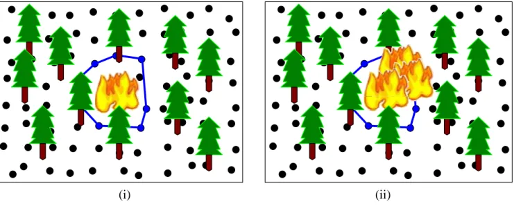
In many applications, events are dynamic and unpredictable. For example in Figure 1.1 (i), the fire may occur somewhere in the forest. Users can know what has happened and where the event is through event detection. However, the forest fire may suddenly bloom at anytime and spread in any direction as depicted in Figure 1.1 (ii). It is important for users to realize when forest fire evolves and the direction it diffuses as soon as possible. Since users can take actions early and thus it minimizes damage or loss.
In order to support the requirements aforementioned, a naive method is to wake up all sensor nodes in the monitoring region for surveillance. However, sensor nodes have rigid energy constraints and die out when they deplete their energies. Due to unattended and untethered
(i) (ii)
Figure 1.1: An example of event surrounding queries in WSN
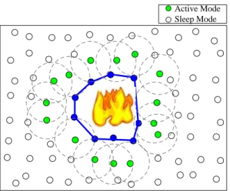
deployment, it is hard to displace sensor nodes in the monitoring region. Therefore, we introduce concepts of surrounding nodes. Surrounding nodes of the event are a set of sensor nodes which are nearest to the event such that no gaps (which are not sensing covered by sensor nodes) exit between adjacent surrounding nodes. If a set of surrounding nodes of the event are selected, sensor nodes in the monitoring region which are not responsible for surveillance can enter into sleep modes temporarily. Thus it can save unnecessary energy consumption and also extend the life time of sensor network. The scenario is demonstrated in Figure 1.2. Surrounding nodes are represented as the center of dashed circles where dashed circles are used to depict sensing ranges. Since surrounding nodes are activated for monitoring event evolution, other sensor nodes can be scheduled to enter into sleep modes to reduce energy consumption.
In order to retrieve surrounding nodes in wireless sensor networks, we propose a novel type of spatial query, Event Surrounding Query (ES Query). Basically, surrounding nodes selection must satisfy two criteria. First, surrounding nodes are sensor nodes which are as close to the event as possible. There is no other sensor nodes nearer than these surrounding nodes selected with regard to the region occupied by their sensing ranges. Thus it can detect event evolution
Active Mode Sleep Mode
Figure 1.2: The usage of surrounding nodes
timely. Second, surrounding nodes must be able to enclose the event. That is, the region between adjacent surrounding nodes must be sensing covered. If there is a gap between two adjacent surrounding nodes, events may spread out in this direction without notification.
Spatial queries, such as Nearest Neighbor Queries [15] (NN Queries), Range Nearest Neigh-bor Query (RNN Query) [10], and Nearest Surrounder Queries [13] (NS Queries), retrieve data based on location information in sensor networks. These type of queries may support us to find out surrounding nodes needed. For example, KNN query [15], which is to retrieve K nearest spatial objects to a given query point. However, it is hard to determine the parameter K for users. If K is too small, sensor nodes in KNN query results cannot enclose the event. If a specified event blooms, it is possible KNN query nodes are not able to detect it timely. We may lose the moment to take essential actions for event diffusion. If K is too large, KNN query results may retrieve nearly all sensor nodes in the monitoring region as surrounding nodes. Although it provides a thorough surveillance, the energy cost of whole sensor network is also large. When given a query range, RNN query [10] will retrieve a set of nearest neighbor nodes to the query range. If we can fit the boundary of the event into a query rectangle, then it can help us to retrieve surrounding nodes potentially. However, the shape of the boundary of the event is not necessarily a query rectangle. Furthermore, although RNN query results
scatter uniformly around the event in contrast to KNN queries, it may not be able to enclose the event, too. In addition, NS queries [13], which retrieve nearest neighbors from a query point at different angles. Different from KNN query and RNN query, NS query results actu-ally enclose the event. However, it is hard to specify such a query point for the event region. Furthermore, NS query is especially suitable for spatial objects of non-zero size. When it is applied to query sensor nodes, since each unique angles are quite small, it may retrieve a lot of sensor nodes in the monitoring region. It will be costly to wake up so many sensor nodes to monitor the event.
In this paper, we study the deficiencies of existent spatial queries and propose two al-gorithms, RNN-ES algorithm and Greedy-ES algorithm, for ES query processing under the environment of sensor networks. We try to extend current research, RNN Query [10]. Al-though RNN query nodes may not enclose the event either as mentioned above, we use some techniques to finish ES query in RNN-ES algorithm. We identify where gaps exit via neighbor-hood relationships first. Then we pick proper sensor nodes to enclose the event. In Greedy-ES algorithm, the position of neighborhood relationships is more important. It not only checks whether surrounding nodes selected enclosing the event but avoids redundant sensor nodes to join the set of ES query results. Moreover, we build a simulation model to evaluate perfor-mances of two proposed algorithms in terms of three parameters, event size, number of query lines, density. Experimental results show that Greedy-ES algorithm outperforms RNN-ES algorithm in CPU time and average number of surrounding nodes selected.
The rest of this paper is organized as follows: Related works are presented in Chapter 2. Chapter 3 is devoted to preliminary. In Chapter 4, two proposed algorithms are described. The performance studies are conducted in Chapter 5. At last, Chapter 6 concludes this paper.
Chapter 2
Related Works
To describe occurrences of events, locations, shapes, and regions they occupied are especially important. Existing works in this area are tend to present this information by event bound-ary. Since the problem of event boundary identification is similar to our surrounding nodes selection. Therefore, we examine related works and discuss differences between surrounding nodes and event boundary.
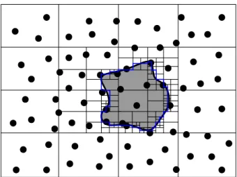
Real boundary computation is complex and accurate boundary estimation requires sensors to consume a lot of energy to communicate, it is better to retrieve approximation boundary than accurate boundary estimation. Nowak et al. [14] propose a method to approximate real boundary and achieve certain accuracy . The authors consider a sensor network are composed of two distinct homogeneous regions. Boundary is a borderline to separate these two regions. To estimate boundary is like edge detection in image processing. The scheme is depicted in Figure 2.1. They use a quadtree-like method to partition the filed to define hierarchy of sensor nodes and obtain finest resolution along the boundary at last. Also, they try to make balance between accuracy and energy consumption.
Another way to approximate real event boundary is through boundary nodes selection. Boundary nodes selection is to select some representative nodes which lie on or near the real boundary. Therefore, these boundary nodes can be approximate to the real boundary and
Figure 2.1: An inhomogeneous field in sensor network
give users conceptual views of events. In [4], a sensor node is viewed as a boundary node if only if a predefined disk center at this sensor contains both sensors in the event and sensors not in the event. Chintalapudi et al. [3] focus on edge detection and defines edge sensors accordingly. If we map the phenomenon of [3] into the event, edge detection can be used to detect boundary. Edge sensors lie in the phenomenon and locate with a specified radius at a borderline which is intersection of interior and exterior of the event. Jin et al. [11] define boundary nodes as sensor nodes which lie within real boundary with certain confidence interval guarantee. According to the definitions introduced, the problem of boundary nodes selection is a problem of classification. Sensor nodes are recognized as boundary nodes or non-boundary nodes. Therefore, the methods proposed above all use statistical methods to differentiate whether sensor nodes are boundary nodes or not.
In sensor networks, sensor nodes may deplete their batteries due to energy constraints and then die out. If there are large amount of sensors die out in sensor networks, we view this as occurrence of a special event. A region, commonly called as a hole, which sensor nodes can not communicate in this region is formulated accordingly. The description of holes estimation is also represented by boundary nodes. The works in [12], [2], [5], [6], and [17] demonstrate how to detect holes and select boundary nodes either topologically or graphically.
Generally, a boundary of an event is just a borderline to separate the event and the remaining monitoring region. Boundary nodes identified may have already involved in the event. Also, if there is any event diffusion, it may not be able to sense at real time because boundary nodes do not necessarily enclose the event. It means that, if we view sensing range as the sensing region which a sensor node can detect variants from the environment. There must be "gaps" exiting between boundary nodes since boundary nodes are merely representative nodes of real boundary approximation. Therefore, the meanings of surrounding nodes are somewhat different from boundary nodes of events.
Chapter 3
Preliminaries
We assume that that each sensor node has a unique id and is aware of their locations via GPS devices or certain positioning methods. Euclidean distance is used as a metric to measure near and far. The deployment of sensor nodes is random and dense enough over a two-dimensional monitoring region. Each sensor nodes has a fixed communication range and a fixed sensing range. The communication range of a sensor node follows unit disk graph model. Therefore, a sensor node si can communicate with a sensor node sj if they are in each others’
communication range. Otherwise, the sensing range of a sensor node is also a disk and smaller than its communication range generally.
The goal of Event Surrounding Query (ES query) is to retrieve a set of nearest surrounding nodes of a specific event. We formally define ES query as follows:
Definition: When given a set of boundary nodes which lie on or near to a real event boundary, an approximate boundary BN of the event can be obtained to bound the event region (generally, BN is a polygon). ES query is to retrieve a set S of nearest sensor nodes to BN such that sensing ranges of adjacent nodes in S must be overlapping to enclose the event. In other words, adjacent sensor nodes si, sj in S, with their sensing ranges ri, rj individually,
root R1 R2 R3 R4 R6 R5 a b c d e h f g A B C D E F q a b c d e f g h R1 R2 R3 R4 R5 R6 (a) (b)
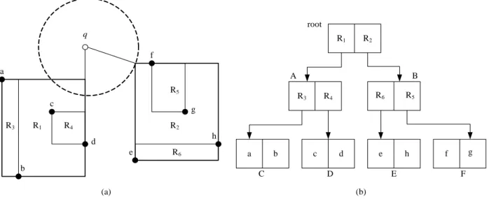
Figure 3.1: Query processing in R-tree
A spatial index structure called R-tree [9] is especially proposed for spatial queries to facilitate query processing. It is a B-tree like index structure. Each leaf nodes has pointers to corresponding spatial objects. Besides, a minimal bounding rectangle (MBR) is a rectangle for a internal node to enlarge least to include all its child nodes. There is an upper bound M and a lower bound m to limit capabilities for a R-tree node to save according objects or child nodes. Basically, R-tree has the following properties: (a) The root node has at least two children unless it is a leaf; (b) A R-tree node contains at least m objects and m satisfy the condition: m ≤ M2; (c) All leaf nodes appear on the same level. If locations of objects are
already known, it is efficient to use R-tree to retrieve spatial objects. Therefore, we also use R-tree to construct a corresponding hierarchy of sensor network topology.
There are two most common search ways of NN: Depth First Search (DFS) [15] and Best First Search (BFS) [8]. Assume a query point q is imposed. DFS starts visiting nodes from the root of R-tree first. It will access R-tree in order of MINDIST which is the minimum distance between the query point and R-tree rectangle. The search process will be repeated until a leaf nodes is visited and the first candidate of nearest neighbor is retrieved. An example is illustrated in Figure 3.1. From the root, MINDIST of R1 is smaller than MINDIST of R2.
of R4 is smaller than R3, the leaf node D of R4is visited and the first nearest neighbor candidate
c is retrieved. MINDIST of current nearest neighbor candidate c is served as local minimum. Then, it will backtrack to upper level parents to check if there are any nodes whose MINDIST are smaller than local minimum of current nearest neighbor candidate. If it does, it may be possible that R-tree nodes which satisfy this property have nearest neighbor. It needs to replace current nearest neighbor candidate if necessarily. The procedure will terminate if there is no MINDIST of r-tree nodes smaller than that of current nearest neighbor candidate so that nearest neighbor is found. In our example, it will backtrack to node A, then the root, and discover that MINDIST of R2 is smaller than current nearest neighbor candidate c. It
compares with MINDIST and follows the path node B, leaf node of R5 and node F. Finally,
nearest neighbor f is retrieved and the search process terminates. Besides, when it talks to BFS, we need to prepare a priority queue in advance. Entries in the priority queue is sorted by their MINDIST to the query point q. BFS pops from top of the queue and check whether it is leaf entry of R-tree or not. If what is popped is not a leaf entry, it will push back into the queue according to the priority, MINDIST. If a leaf entry is popped, it becomes nearest neighbor. In previous example, it will traverse r-tree node R1 first, then follow the sequence
of R2, R5 in the priority queue. At last, the leaf entry is popped and nearest neighbor f is
Chapter 4
Algorithms for Event Surrounding
Queries
In this chapter, we propose two algorithms for ES query processing. The first algorithm we propose tries to extend an input query rectangle of RNN query to a polygon. We find out range nearest neighbor nodes of an approximate polygonal region of the event first. Then we try to enclose the event with helps of RNN ’s neighbors. The second algorithm is a Greedy algorithm. Every time we select from nearest neighbor nodes as our surrounding nodes of the event.
4.1
RNN-based Algorithm: RNN-ES
4.1.1
Overview
RNN-ES algorithm consists of two phases: initial phase and enclosure phase. Initial phase is to selects RNNs as our basic components of surrounding nodes. Enclosure phase is to identify where gaps exit between surrounding nodes and then try to select proper surrounding nodes for enclosing the event. Besides, there is a running example that demonstrates how to select
sensor nodes to enclose the event as described in enclosure phase.
4.1.2
Initial Phase
There have been many methods proposed for event boundary detection till now and sensor nodes are recognized as boundary nodes by these algorithm. Therefore, we can facilitate from these methods to obtain boundary nodes of the event. To compute approximate polygonal boundary of the event boundary is similar to compute a convex hull by GRAHAM’s SCAN [7].
Furthermore, we observe that range nearest neighbor sensor nodes are parts of surrounding nodes. If we view an approximate polygonal event boundary as a range, we can solve our problem with helps of RNN query [10]. However, RNN query proposed processes a query rectangle only. The event region is determined by what has happened in the environment. The polygonal boundary of approximate event boundary is not necessarily a rectangle. Therefore, We want to extend the query range of RNN query to a polygonal region. Then, the polygon of approximate event boundary can be divided into several lines that each line is corresponding to a polygonal edge. We look for LNNs for each lines. A line can be partitioned into several subsegments further and each subsegment corresponds to a LNN. Because a line can be divided into finite and minimal sets of subsegments, adjacent subsegments must have different NN as described in [10].
Tao et al. [16] propose a method to process LNN Search. It can apply either BFS or DFS search paradigms of R-tree. Take BFS for example, a priority queue is prepared to store the entries in order of MINDIST. When a leaf entry is popped, corresponding sensor nodes are push back to the priority queue. Thereafter, we can pop the priority queue and access sensor nodes that are possible NNs. In order to differentiate different segments of
Algorithm 1 RNN-ES(BN,root)
Input: An approximate polygonal event boundary (BN), and A R-tree root index node(root). Output: A set of surrounding nodes of the event S.
1: Let Q be a priority queue and be initialized with root;
2: Let S be results of ESN Query and be initialized φ;
3: Let d(ei,ei.NN) be the distance between an endpoint ei and its LNN and initialized as ∞;
4: Let EXMAX be the maximum distance, d(ei,ei.NN), of EL and initialized as ∞;
5: Let start be the start endpoint of a query line Li and its LNN, start.NN, initialized as
null;
6: Let end be the end endpoint of a query line Li and its LNN, end.NN, initialized as null;
7: Let EL be the endpoint set of a query line Li that it can divide Li into several subsegments
through these endpoints. Initial EL:(start, end);
8: Let Ecover be a set of the endpoints covered by the spatial object n and be initialized φ;
9: for each query line Li of BN do
10: while(Q is not empty) do
11: Dequeue node n from Q;
12: if (n is a spatial object) then
13: if (MINDIST(n,Li) < ELMAX) then
14: //all LNNs of endpoints of EL are null
15: if (start.NN and end.NNs are both null) then
16: Update start.NN and end.NN as n;
17: Update d(start,start.NN);
18: Update d(end, end.NN);
19: Update ELMAX;
20: end if
21: else
22: if (Ecover is not empty) then
23: Remove endpoints covered by n from EL;
24: end if
25: // Ecover:{ei,ei+1,. . . ,ej}
26: Let u=ei−1.NN;
27: Let u=ej.NN;
28: Add an endpoint e0i into EL by doing perpendicular bisector of n,u with Li;
29: Update d(e0
i, e0i.NN);
30: Add an endpoint e0
i+1 into EL by doing perpendicular bisector of n,v with Li;
31: Update d(e0i+1, e0i+1.NN) ;
32: Update ELMAX;
33: Clear Ecover set;
34: end if
35: else
36: if (MINDIST(n,Li) < ELMAX) then
37: if (An endpoint ek in EL exits such that d(ek,ek.NN) > MINDIST(ek,n)) then
38: foreach child entry c of n do
39: Enqueue node c; 40: end for 41: end if 42: end if 43: end if 44: end while
45: Dump all LNNs of endpoints of EL into S;
○30 ○27 ○34 ○60 ○47 ○39 ○61 ○50 ○59 ○55 ○62 ○42 ○21 BN Figure 4.1: RNN example
doing the intersection between a perpendicular bisector of current scanned nodes, neighboring LNN nodes and L. Thus, for each endpoints ei which belong to the query line L, all points
of L in [ei,ei+1] has the same NN defined as ei.NN. It is possible that sensor nodes scanned
later are much closer than sensor nodes for certain subsegments in the LNN list. Therefore, it needs to check whether this sensor node covers some endpoints which are obtained by nodes previously scanned. If there is a currently scanned sensor sj whose distance dist(sj,ei)
is smaller than dist(ei,ei.NN) for some ei, it means the endpoint ei is covered by sj. Since
there are endpoints of subsegments obtained from intersection of the perpendicular bisector and the specified query line, the currently scanned sensor sj is LNN. The algorithm proposed
removes the endpoint ei, adds new endpoints e0i by sj and updates e0i.NN accordingly. Also, a
threshold ELMAX which determines the number of surrounding node candidates visited needs to be updated as maximum d(ek,ek.NN) of current LNN list. Finally, we prepare a queue S to
gather the results of LNN lists and sort them counterclockwise (or clockwise) with reference to the center of the approximate polygonal boundary of the event. These will be parts of selection of our surrounding nodes of the event (Figure 4.1). Next phase we will introduce how we select nodes to enclose the event with helps of RNNs obtained from this phase.
4.1.3
Enclosure Phase
Algorithm 2 RNNEnclosure(S)
Input: A queue S which contains RNN results. Output: A set of surrounding nodes of the event S.
1: for all si in S do
2: if (!(dist(si,si.left) < rsi+rsi.lef t )) then
3: choose sk from si’s and si.left’s adjacency list with Min(dist(si,sk)+dist( sk,si.left))
4: sk.left=si.left;
5: sk.right=si;
6: (si.left).right=sk;
7: si.left=sk;
8: Insert sk at the end of S;
9: else if (!(dist(si,si.right) < rsi+rsi.right )) then
10: choose sk from si’s and si.right’s adjacency list with Min(dist(si,sk)+dist( sk,si.right))
11: sk.left=si;
12: sk.right=si.right;
13: (si.right).left=sk;
14: si.right=sk;
15: Insert sk at the end of S;
16: else
17: ;
18: end if
19: end for
In prior phase, we have already retrieved partial results of nearest surrounding nodes of the event and push them in a queue S either clockwise or counterclockwise. Then, we construct neighborhood relationships for each sensor node in S first. If we sort nodes in the queue S counterclockwise with reference to the center point of the approximate polygonal boundary of the event, a sensor node si indexed i in the queue S sets its left-hand side neighbor as a
sensor node indexed i+1 and its right-hand side neighbor as a sensor node indexed i-1 in the queue S. A special case is that a sensor node at the head of the queue S will set its right-hand side neighbor as a sensor node at the end of the queue S and the sensor node at the end of the queue S will set its left-hand side neighbor as the sensor node at the head of the queue S accordingly. If we sort nodes in the queue S clockwise, neighborhood relationship construction will be in a similar manner. Because we only have partial results of nearest surrounding nodes of the event in prior phase and these sensors are too few to enclose the event, there may be
gaps between adjacent nodes with respect to their sensing ranges. The goal of this phase is to select proper sensors to enclose the event. The requirement for this phase is that each sensor node needs to keep information of their one-hop neighbors. Therefore, each sensor node has to store its neighbors within communication range in its adjacency list. Then, the algorithm proposed starts to access the queue S and checks whether gaps exit between this node and its adjacent neighbors in S. When a sensor node si in S is accessed, it first checks the distance
between this sensor and its left-hand side neighbor si.left. If the distance, d(si,si.left), is greater
than summation of sensing radius of si (rsi) and its left-hand side neighbor si.left (rsi.left), it
means that there is a gap between them. We select from the set of neighbors in adjacency lists of si and si.left. A neighbor node sk in adjacency lists selected as surrounding nodes must
satisfy the condition that: it has minimum distance which is summation of distances from sk
to si and sk to its si.left. If there is a tie, it will choose one of sk arbitrarily as surrounding
nodes. We also construct neighborhood relationship for sk as to two neighbors, si and si.left.
Accordingly, sk will replace original position of si.left and become new left-hand side neighbor
of si. Original right-hand side neighbor of si.left will be sk. Then, sk will be insert at the
end of the queue S. Similarly, it will also checks whether there is a gap between si and si’s
right-hand side neighbor, si.right, and select proper skto enclose it. This process will continue
until all elements in S have been checked. At last, we report all sensor nodes in S as nearest surrounding nodes of the event.
4.1.4
Running Example of RNN-ES algorithm
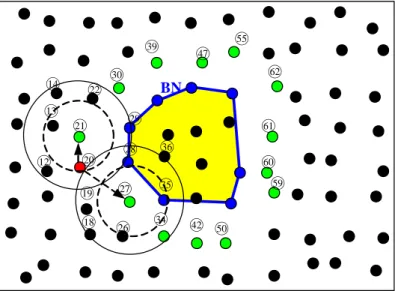
An example of surrounding nodes selection for event enclosure is illustrated in Figure 4.2. The approximate polygonal event boundary is a octagon. For each sensor, it has a communication range of 6 m and a sensing range of 4 m. A sensing range of a sensor is represented by a dashed circle and a communication range of a sensor is represented by a solid circle. Initially,
surrounding nodes selected from the first phase have already sorted counterclockwise and construct neighborhood relationship with adjacent neighboring nodes such as 21 and 27 in Table 4.1. Therefore, a node numbered 21 has a left-hand side neighbor node 27 and a right-hand side neighbor node 30. A node numbered 27 has a left-right-hand side neighbor node 34 and a right-hand side neighbor node 21. When the node 21 is accessed from the queue S, it discovers that the distance between the node 21 and its left-hand side neighbor node 27 is greater than summation of sensing radius of the node 21 and the node 27. To enclose the event, the algorithm proposed will examine adjacency lists in the node 21 and its left-hand side neighbor node 27 and select a proper node as a surrounding node. In the adjacency list of the node 21, it has six neighbor nodes: 12, 13, 14, 20, 22, and 29. In the adjacency list of the node 27, it also has six neighbor nodes: 18, 19, 26, 28, 34, and 35. Among these neighbors, the node 20 has minimal summation distance to the node 21 and the node 27. We construct neighborhood relationship for the node 20 with the node 21 and the node 27 individually. Besides, we modify the neighborhood relationship for the node 21 and the node 27 accordingly (As Table 4.2 depicted). Then, the node 20 is inserted at the end of the queue S. We go on to check whether there is a gap between the node 21 and its right-hand side neighbor, the node 30. Because the distance between the node 21 and its right-hand side neighbor, the node 30, is smaller than summation of sensing radius of the node 21 and node 30, there is no gap between the node 21 and the node 30. The algorithm continues to check next sensor in the queue S until it retrieves a set of nearest surrounding nodes enclosing the event.
Node si si.left si.right
21 27 30
27 34 21
○30 ○27 ○34 ○60 ○47 ○39 ○61 ○50 ○59 ○55 ○62 ○42 ○21 ○20 ○18 ○19 ○26 ○36 ○12 ○13 ○22 ○14 ○28 ○29 ○35 BN
Figure 4.2: Surrounding nodes selection for enclosure
4.2
Greedy Algorithm: Greedy-ES
4.2.1
Design Concepts
Although it is intuitive to select surrounding nodes of the event by RNN-ES algorithm, there are some deficiencies in RNN-ES algorithm. It may be costly to search RNNs edges by edges. Also, RNN-ES algorithm requires that each sensor node caches neighbor nodes in its communication range in case of RNNs selected not enclosing the event. Therefore we propose a greedy algorithm for ES query processing and it is abbreviated as Greedy -ES.
In our Greedy-ES algorithm, we need to calculate minimum distance between sensor nodes to the approximate polygonal boundary of the event boundary. Then we select from near-est neighbor nodes of the approximate polygonal boundary of the event every time as our surrounding node candidates. The search process will stop until we find a set of nearest surrounding nodes of the event that enclose the event.
Node si si.left si.right
20 27 21
21 20 30
27 34 20
When we takes two search schemes mentioned of R-tree index structure, BFS and DFS, into consideration, we choose BFS search paradigm according to the essence of our Greedy algorithm. The definition of minimum distance of a sensor node to the approximate polyg-onal event boundary is similar to MINDIST defined in [15]. If the approximate polygpolyg-onal event boundary is inside MBR of R-tree fully, minimum distance is zero. If the approximate polygonal event boundary covers partial region of MBR, minimum distance is also zero. If the approximate polygonal event boundary is outside MBR fully, minimum distance is the minimal Euclidean distance between the node to nearest edge of the approximate polygonal event boundary. We use minimum distance defined to sort nodes in our priority queue for BFS search paradigm. Conceptually, we retrieve NN of current processing as our surrounding nodes by popping the priority queue. However, not all K NNs searched accessed till now are surrounding nodes of the event. It may be redundant for current NN retrieved to join the set of surrounding nodes of the event. Therefore, we introduce how to construct neighborhood relationships for each surrounding node candidates NN and current ES results.
In our assumption, nearest surrounding nodes that enclose the event must satisfy the criteria, sensing ranges of adjacent surrounding nodes are overlapping. Distances between every two adjacent surrounding nodes is small than the summation of their radius of sensing ranges. Therefore, we check the distance between each surrounding nodes candidates NN and current ES results. If a surrounding nodes candidate NN retrieved satisfy the criteria, NN has neighborhood relationship with current ES results. Next, we define left-hand side neighbor and right-hand side neighbor for a surrounding node candidate NN advancedly.
Neighborhood relationships construction of a surrounding node candidate is depicted in Figure 4.3. We mark current surrounding node candidate processed as si. Sensor nodes sj,
sk are surrounding nodes and have been recognized as neighborhood of si by the criteria
aforementioned. We set center point of the approximate polygonal event boundary as a reference point. If there is a polar angle formed by the reference point, the surrounding node
Algorithm 3 Greedy-ES(BN,root)
Input: An approximate polygonal event boundary (BN), and A R-tree root index node(root). Output: A set of surrounding nodes of the event S.
1: Let Q be a priority queue and be initialized with root;
2: Let S be results of ESN Query and be initialized φ;
3: Let Mark be a redundant surrounding nodes mark if n is added to S and be initialized 0;
4: while (Surrounding nodes in S are not enclosed or S==φ) do
5: Dequeue node n from Q;
6: if (n is a spatial object) then
7: n.left = null;
8: n.right = null;
9: if (S != φ) then
10: foreach nodes si in S do
11: if (dist(n,si) ≤ rn+rsi) then
12: Build neighborhood relationships for n such as n.left = si or n.right = si;
13: end if
14: end for
15: end if
16: if ((n.left==si) and (si.right==null)) then
17: si.right = n;
18: else if ((n.right==si) and (si.left==null)) then
19: si.left = n;
20: else if ((n.left==si) and (si.right != null) and (si.right != n)) then
21: Mark = 1;
22: break;
23: else if ((n.right==si) and (si.left != null) and (si.left != n) then
24: Mark = 1; 25: break; 26: end if 27: if (Mark == 0) then 28: S = S ∪ n; 29: else
30: Mark = 0; //reinitialize Mark as 0
31: end if
32: else
33: for each child node ci of n do
34: Enqueue(ci);
35: end for
36: end if
37: end while
s
is
js
k BNFigure 4.3: The neighborhood relationships among surrounding nodes
candidate si, a neighbor of si in current ES result sj, sj is a left-hand side neighbor of the
surrounding node candidate si. This means that if the surrounding node candidate in Figure
4.3 is si, si to si’s neighbor, sj, makes counterclockwise turn relative to the reference point, sj is
si’s left-hand side neighbor. Similarly, if there is a solar altitude angle formed by the reference
point, the surrounding node candidate si, a neighbor of si in current ES result sk, sk is a
right-hand side neighbor of the surrounding node candidate si. In Figure 4.3, the surrounding
node candidate si to si’s neighbor, sk, makes clockwise turn relative to the reference point.
Thus, sk is si’s right-hand side neighbor.
We construct such neighborhood relationship for each surrounding node candidate and initialize their left-hand side and right-hand side neighbor as null first in our Greedy-ES algorithm. Then , it will go on to check whether there any surrounding nodes in current ES result set are its neighbors. If there is none, it will join current ES result set directly and continue the procedure. If it has neighbors in current ES result set, it will examine this neighbor belongs to left-hand side or right-hand side neighbor advancedly. In order to avoid redundant surrounding nodes to join ES result set, we will check neighborhood relationships of each surrounding node candidate and its corresponding neighbors in ES result set. There
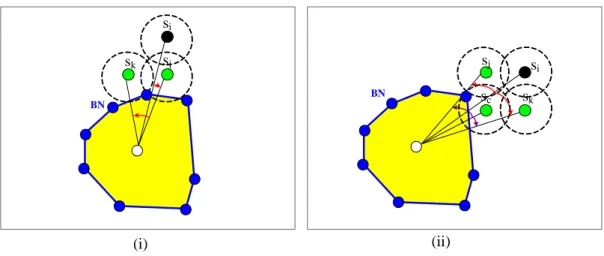
si sj sk sj si sk (i) (ii) sc BN BN
Figure 4.4: (i) Case 1. and (ii) Case 2.
are two cases that surrounding node candidates are redundant (See Figure 4.4):
Case1. The sensing range of a surrounding node candidate si is overlapping with an
element sj in ES result set, and sj is si’s right(left)-hand side neighbor. But sj’s according
left(right)-hand side neighbor is sk. This means the role of current surrounding node candidate
is already played by sk and si is farther than sk. We avoid si to join the ES result set.
Case 2. The sensing range of a surrounding node candidate si is overlapping with two
elements sj and sk in ES result set. sj is si’s left(right)-hand side neighbor and sk is si’s
right(left)-hand side neighbor. But sj’s right(left)-hand side neighbor and sk’s
left(right)-hand side neighbor are sc not si. This can just use case 1 to check whether neighborhood
relationships of a surrounding node candidate exits or not. There is no need to check twice. Therefore, if surrounding node candidate si’s left(right)-hand side neighbor is sj in ES result
set and sj’s according right(left)-hand side neighbor is null. This means that surrounding node
is not redundant to enclose the event. We construct corresponding neighborhood relationship of si and sj and add si into our ES result set. Thereafter, we avoid redundant surrounding
R1 R2 R3 R4 R5 R6 R7 R8 R9 R10 R11 R12 R13 R14 R15 R16 R17 R18 R19 R20 BN
Figure 4.5: R-Tree index structure
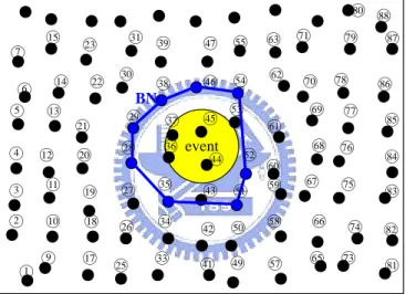
event ○1 ○2 ○3 ○4 ○5 ○6 ○7 ○9 ○10 ○11 ○12 ○13 ○14 ○15 ○17 ○18 ○19 ○20 ○21 ○22 ○23 ○25 ○26 ○28 ○29 ○30 ○31 ○27 ○33 ○35 ○36 ○37 ○38 ○34 ○39 ○41 ○42 ○43 ○44 ○45 ○46 ○47 ○49 ○50 ○51 ○52 ○53 ○54 ○55 ○57 ○58 ○59 ○60 ○61 ○62 ○63 ○65 ○66 ○67 ○68 ○69 ○71 ○70 ○73 ○74 ○75 ○76 ○77 ○78 ○79 ○80 ○81 ○82 ○84 ○88 ○83 ○85 ○86 ○87 BN
Figure 4.6: Before processing
○27
BN
○27
○60
○47
○30
BN
Figure 4.8: Processing a surrounding node candidate 30
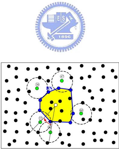
○27 ○60 ○47 ○30 ○34 BN
4.2.2
Running Example of Greedy-ES algorithm
The search process of our greedy algorithm is shown from Figure 4.5 to Figure 4.10. The center point of the approximate polygonal event boundary is represented as a white point in these figures and serves as a reference point. The root of R-tree has already been enqueued in our greedy algorithm. By BFS search paradigm, we has a priority queue Q to sort nodes by their minimum distance to the approximate polygonal event boundary. We dequeue the root node of R-Tree first and discover that it is not a spatial object (i.e. a sensor node here). Therefore, we push its children R1, R2, R3 back to the priority queue Q. Since the MINDIST
to the approximate polygonal event boundary BN of R2 = R3 < R1, they are located in
Q in this order. We go on the push and pop procedure until we retrieve the first NN, the sensor node numbered 27 in Figure 4.7. We initialize left-hand side neighbor and right-hand side neighbor of the sensor node 27 as null individually. Then, we check whether it has any neighbor nodes in current surrounding node set. Since the sensor node 27 is the first NN , there is no surrounding nodes selected in current surrounding node set yet. Therefore, the sensor node 27 has no adjacent surrounding node neighbors now and join current surrounding node set S directly. Similarly, sensor nodes numbered as 60, 47, 30 in Figure 4.8 perform the same procedure sequentially. They all have no left-hand side neighbor and right-hand neighbor yet and join surrounding node set S directly. The next NN, a spatial object popped from the queue Q, is a sensor node numbered as 34. We also initialize its left-hand side neighbor and right-hand side neighbor as null. Then, we find that the sensor node 34 is neighboring to a surrounding node, the sensor node numbered as 27, and makes right turn to it according to the reference point (Figure 4.9). Therefore, the surrounding node candidate 34 has a right-hand side neighbor 27. We check whether the surrounding node 27 has a left-hand side neighbor. Since the left-hand side neighbor of the surrounding node 27 is null, the surrounding node candidate 34 is not redundant to enclose the event. We modify neighborhood relationships
○30 ○27 ○34 ○60 ○47 ○39 ○61 ○50 ○59 ○55 ○62 ○20 ○22 BN
Figure 4.10: Nearest surrounding nodes
of the surrounding node 27 and the surrounding node candidate 34 accordingly. Then, we recognize the sensor node 34 as a surrounding node and add it to our surrounding node set S. The procedure will repeat until we find out a set of nearest surrounding nodes to enclose the event so that there are no surrounding nodes whose left-hand side neighbor or right-hand side neighbor are null. Finally, the results are shown in Figure 4.10.
Chapter 5
Performance Study
In this chapter, we evaluate the performance of two proposed surrounding nodes selection algorithms, Greedy-ES algorithm and RNN-ES algorithm.
5.1
Simulation Model
Experiments are implemented in Java programming language and run on a computer with 64 X2 Dual Core Processor 3800+ and 2 G memory. There are 2500 sensor nodes deployed in our monitoring region. For each sensor node, its sensing range is fixed at 4 m and communication range is fixed at 8 m. A variant of R-tree index structure, R∗-tree [1], is used to index
sensor nodes and speeds up sensor nodes retrieval. The pagesize of one R∗-tree node is set
to 4096 bytes and maximum node capacity is 50. We assume that an event occurs in the monitoring region. The shape of the event is a circle. The boundary nodes of the event have already collected. The approximate polygonal boundary of the event can be obtained via the boundary nodes of the event. We use synthetic datasets to simulate the deployment of sensor nodes. The deployment of sensor nodes must be dense enough so that we can find out surrounding nodes of the event. Two kinds of deployment, grid distribution and grid with random perturbation distribution, are applied individually for comparison. There are two
metrics used to compare the performance of proposed methods which are described as follows: (1)CPU time for surrounding nodes selection (2)Numbers of surrounding nodes of the event.
5.2
The Impact of Event Size
We vary the size of the event through varying its radius from 4m to 28 m without changing its center. The monitoring region is assumed to be 200 m × 200 m. We deploy 2500 sensor nodes so that each sensor node can be put in a 4 m × 4 m grid. Because it is a grid distribution of sensor nodes, the environment is simple. The edges of the approximate polygonal boundary of the event in this case are always 4. Figure 5.1 shows the simulation result of varying the size of the event. As our expectation, when we increase the size of the event, the cost to find out surrounding nodes of the event will raise accordingly. Since RNN-ES algorithm needs to search RNNs edges by edges according to the approximate polygonal boundary of the event, the cost of RNN-ES algorithm is essentially higher than Greedy-ES algorithm. Furthermore, Figure 5.2 demonstrate numbers of surrounding nodes of the event. In this case, the numbers of surrounding nodes retrieved by both methods are the same.
In order to be contrast to the grid deployment of sensor nodes, a group of control is shown in Figure 5.3 and Figure 5.4. We deploy sensors randomly instead. Sensor nodes are put in a grid and then perturbed with a random shift. Therefore, the distribution of sensor nodes by manual will be close to uniform distribution. The event size also increases by adjusting the radius of the event from 4 m to 28 m. Therefore, the numbers of edges of the approximate polygonal boundary which vary with the size of the event accordingly are as follows: 6, 9, 16, 14, 21, 21, 23. Generally, the cost of RNN-ES algorithm is higher than Greedy-ES algorithm in Figure 5.3 . This is similar to the scheme of the grid deployment of sensor nodes. However, there is somewhat a little oscillation of the RNN-ES algorithm curve in Figure 5.3. When the
0 0.1 0.2 0.3 0.4 0.5 28 24 20 16 12 8 4 CPU Time(sec) Event Radius(m) Greedy-ES RNN-ES
Figure 5.1: Grid deployment: event size vs. CPU time
10 20 30 40 50 60 70 28 24 20 16 12 8 4
Number of Surrounding Nodes
Event Radius (m)
Greedy-ES RNN-ES
0 0.5 1 1.5 2 2.5 3 28 24 20 16 12 8 4 CPU Time(sec) Event Radius(m) Greedy-ES RNN-ES
Figure 5.3: Random deployment: event size vs. CPU time
10 15 20 25 30 35 40 45 50 55 28 24 20 16 12 8 4
Number of Surrounding Nodes
Event Radius (m)
Greedy ES RNN-ES
than its previous one and the next one of event size. Therefore, it costs less overhead to search RNNs in the first phase of RNN-ES algorithm. Since the first phase of RNN-ES algorithm incurs major cost of RNN-ES algorithm, it costs less totally at last. Otherwise, although the number of edges of the approximate polygonal boundary when the radius of the event is 20 m is the same as that when the radius of the event is 24 m, the cost to retrieve surrounding nodes is less in RNN-ES algorithm when the radius of the event is 24 m. Because it visits more surrounding candidates when the radius of the event is 24 m. And this is due to the distribution of surrounding node candidates around the approximate polygonal boundary. It will discuss further latter in next section. Figure 5.4 presents the scheme of ES query in the random deployment environment. We observe that RNN-ES algorithm most often retrieves more sensor nodes than Greedy-ES algorithm. Since RNN-ES algorithm searches RNNs by dividing the approximate polygonal boundary into several query lines in the first phase, a query line L must be divided into segments further until that no NN candidates can cover current set of LNNs. This property causes the number of surrounding nodes selected by RNN-ES algorithm to be less than or more than or equal to Greedy-ES algorithm. Moreover, Greedy-ES algorithm is tend to select representative nearest surrounding nodes as long as nodes selected can enclose the event.
5.3
The Impact of Number of Query Lines
As aforementioned in the first phase of RNN-ES algorithm, it breaks the approximate polygo-nal boundary into several query lines for RNN search. It is probably that the number of query lines will influence the query cost of RNN-ES algorithm. To show the impact of the number of query lines, we simulate and present the result in Figure 5.5. Sensor nodes are deployed in a 4 m × 4 m gird and perturbed with a random shift. The radius of the circular event is fixed at 8 m and we assume that it occurs arbitrarily in the monitoring region so that we
0 0.2 0.4 0.6 0.8 1 14 13 12 11 10 9 CPU Time(sec)
Number of Query Lines
Greedy-ES RNN-ES
Figure 5.5: Random deployment: no. of query lines vs. CPU time
obtain different number of edges of the approximate polygonal boundary. Naturally, it has no much effect for Greedy-ES algorithm if the event occurs anywhere in the monitoring region in Figure 5.5. However, RNN-ES algorithm is tend to increase its CPU time as the number of the query line of the approximate polygonal boundary increases. We also observe that CPU time descends when the number of query lines of the approximate polygonal boundary is 10. Due to the distribution of sensor nodes around the approximate polygonal boundary, it will determine the number of surrounding node candidate to traverse in the search process. That is, for a query line L, nodes in current LNN set will determine the threshold ELMAX which chooses to visit more surrounding nodes candidates or not. Therefore, the threshold is more powerful to decide the number of surrounding node candidates visited than the number of query lines of the approximate polygonal boundary.
The corresponding number of surrounding nodes selected is depicted in Figure 5.6. RNN-ES algorithm often selects more surrounding nodes than Greedy-RNN-ES algorithm as above-mentioned. The difference of number of surrounding nodes selected is not too much in this
15 16 17 18 19 20 21 22 14 13 12 11 10 9
Number of Surrounding Nodes
Number of Query Lines
Greedy-ES RNN-ES
Figure 5.6: Random deployment: no. of query lines vs. no. of surrounding nodes case since the radius of the event is the same.
In order to show the impact of the distribution of surrounding node candidates around the approximate polygonal boundary more precisely, we collect and simulate the same number of query lines of the approximate polygonal boundary to evaluate the query cost. The radius of a event is also fixed at 8 m and the deployment of sensor nodes is the same as the envi-ronment depicted in Figure 5.5 and Figure 5.6. Although events may occurs anywhere in the monitoring region, we only focus on the events which have the same number of query lines of the approximate polygonal boundary that we collect the events whose number of query lines is 11. Figure 5.7 demonstrates the result. The curve of RNN-ES algorithm is almost smooth. However, there is still some rise and fall at the end of the curve. The distribution of sur-rounding node candidates around the approximate polygonal boundary leads to the variation apparently. Greedy-ES algorithm also displays a slightly fluctuation due to the distribution of surrounding node candidates around the approximate polygonal boundary but the range of variation is small. We also present the corresponding number of surrounding nodes selected
0 0.1 0.2 0.3 0.4 0.5 0.6 0.7 0.8 7 6 5 4 3 2 1 CPU Time(sec) Sample Greedy-ES(QL:11) RNN-ES(QL:11)
Figure 5.7: Random deployment: no. of query lines is fixed as 11 vs. CPU time
15 16 17 18 19 20 21 7 6 5 4 3 2 1
Number of Surrounding Nodes
Sample
Greedy-ES(QL:11) RNN-ES(QL:11)
Figure 5.8: Random deployment: no. of query lines is fixed as 11 vs. no. of surrounding nodes
in Figure 5.8. Since the radius of the event is the same and we select the events of the same number of query lines, the difference of the number of surrounding nodes is not too much in both methods. Otherwise, RNN-ES algorithm also selects more surrounding nodes than Greedy-ES algorithm at most of times.
5.4
The Impact of Density
Generally, density in sensor networks is defined as: The Number of Sensor Nodes DeployedMonitoring region size . In order to show the impact of density, we fix the number of sensor nodes deployed as 2500 and vary the size of monitoring region as 200 m × 200 m, 100 m × 100 m, 50 m × 50m , 25 m × 25 m instead. Sensor nodes deployed follow grid distribution. A circular event whose radius is 8 m occurs in the center of the monitoring region. In Figure 5.9, the cost to select surrounding nodes increases along with density raising in both methods. However, RNN-ES algorithm not only consumes more CPU time but its direction of curve increases more rapidly than Greedy-ES algorithm. This is because surrounding candidates which satisfy the threshold in RNN-Greedy-ES algorithm will increase relatively when density grows. Therefore, RNN-ES algorithm needs to examine more surrounding candidates than Greedy-ES algorithm.
Figure 5.10 shows the number of surrounding nodes selected by proposed methods if we vary density under the environment mentioned above in Figure 5.10. It is observed that RNN-ES algorithm most often is tend to retrieve more sensor nodes with density increasing. Moreover, the difference of the number of surrounding nodes selected is larger and larger be-tween RNN-ES algorithm and Greedy-ES algorithm when density increases. This is probably due to that Greedy-ES algorithm is tend to select representative nearest surrounding nodes as aforementioned. In contrast to Greedy-ES algorithm, RNN-ES algorithm takes a different viewpoint. Most of surrounding nodes selected by RNN-ES algorithm is done in the first phase. Therefore, RNN-ES algorithm select RNNs by definition of LNNs and the RNN set is
0 0.5 1 1.5 2 2.5 3 3.5 25x25 50x50 100x100 200x200 CPU Time(sec)
Monitoring Region Size(m2) Greedy-ES
RNN-ES
Figure 5.9: Grid deployment: density vs. CPU time
0 20 40 60 80 100 120 140 160 25*25 50*50 100*100 200*200
Number of Surrounding Nodes
Monitoring Region Size (m2) Greedy-ES
RNN-ES
composed of several different LNN sets. Since the search must continue until the query line of the approximate polygonal boundary can not be divided into segments by surrounding node candidates, surrounding nodes retrieved by RNN-ES algorithm are like a second boundary of the event. Therefore, when density of the monitoring region increases, it is tend to be more surrounding nodes candidates involved and covers current surrounding nodes selected in the search process. Thus, the difference of the number of surrounding nodes between RNN-ES al-gorithm and Greedy-ES alal-gorithm enlarges accordingly. Especially the number of surrounding nodes selected by Greedy-ES algorithm does not vary too much.
Chapter 6
Conclusion
In this paper, we presented a novel type of spatial query, ES Query, for application require-ment in sensor networks. Through ES Query, We can select a set of surrounding nodes of the event instead of all sensor nodes in the monitoring region to check if there is any event evolution. Therefore, sensor nodes which are not surrounding nodes can enter into sleep modes temporarily to save their battery energies and thus extend the lifetime of sensor net-works.Furthermore, to reply ES query, we proposed two algorithm, RNN-ES algorithm and Greedy-ES algorithm. RNN-ES algorithm derives from the concept of RNN and makes an extension to enclose the event. However, RNN-ES algorithm takes a microscopic view and breaks the approximate polygonal event boundary into several query lines for LNN search. Although surrounding nodes selected around the event may follow a homogenized distribution, it is costly to search LNNs line by lines. Besides, experimental result showed that the number of surrounding nodes selected is tend to be more and it will increase rapidly especially when the density of sensor deployment increases. Therefore, Greedy-ES algorithm was proposed to reply ES Query efficiently. Greedy-ES algorithm takes a macroscopic view and regards the approximate polygonal event boundary as a whole query input. It greedily visits NN candi-dates until surrounding nodes selected encloses the event. The core of Greedy-ES algorithm
redundant to join the set of surrounding nodes of the event or surrounding nodes selected so far enclosing the event or not.
Bibliography
[1] N. Backmann, H.-P. Kriegel, R. Schneider, and B. Seeger. The R*-tree: An Efficient and Rrobust Access Method for Points and Rectangles. In Proceedings of the 9th ACM International Conference Management of Data (SIGMOD), pages 322—331, 1990.
[2] K. Bi, K. Tu, N. Gu, W. Dong, and X. Liu. Topological Hole Detection in Wireless Sensor Networks and its Applications. In Proceedings of 2006 International Conference on Systems and Networks Communication (ICSNC), pages 31—31, 2006.
[3] K. K. Chintalapudi and R. Govindan. Localized Edge Detection in Sensor Fields. In Proceedings of the 1st IEEE International Workshop on Sensor Network Protocols and Applications (SNPA), pages 59—70, May 2003.
[4] M. Ding, D. Chen, K. Xing, and X. Cheng. Localized Fault-Tolerant Event Boundary Detection in Sensor Networks. In Proceedings of the 24th IEEE International Conference of Computer and Communications Society (INFOCOM), March 2005.
[5] Q. Fang, J. Gao, and L. J. Guibas. Locating and Bypassing Routing Holes in Sensor Networks. In Proceedings of the 23th IEEE International Conference of Computer and Communications Society (INFOCOM), 2004.
[6] S. Fekete, M. Kaufmann, A. Kröller, and K. Lehmann. A New Approach for Bound-ary Recognition in Geometric Sensor Networks. In Proceedings of the 17th Canadian
[7] R. Graham. An Efficient Algorithm for Determining the Convex Hull of a Finite Planar Set. Information Processing Letters (IPL), 1(4):132—133, 1972.
[8] G.R.Hjaltason and H. Samet. Distance Browsing In Spatial Databases. ACM Transaction on Database Systems(TODS), 24(2):265—318, 1999.
[9] A. Guttman. R-trees: a dynamic index structure for spatial searching. In Proceedings of the 3rd ACM International Conference on Management of Data (SIGMOD), pages 47—57, 1984.
[10] H. Hu and D. L. Lee. Range Nearest Neighbor Query. IEEE Transactions on Knowledge and Data Engineering (TKDE), 18(1):78—91, 2006.
[11] G. Jin and S. Nittel. NED: An Efficient Noise-Tolerant Event and Event Boundary Detection Algorithm in Wireless Sensor Networks. In Proceedings of the 7th International Conference on Mobile Data Management (MDM), pages 153—153, 2006.
[12] A. Kröller, S. P. Fekete, D. Pfisterer, and S. Fischer. Deterministic Boundary Recognition and Topology Extraction for Large Sensor Networks. In Proceedings of the 17th ACM-SIAM Symposium on Discrete Algorithm (DA), pages 1000—1009, 2006.
[13] K. C. K. Lee, W.-C. Lee, and H. V. Leong. Nearest Surrounder Queries. In Proceedings of the 22nd IEEE Internationl Conference on Data Engineering (ICDE), page 85, 2006.
[14] R. Nowak and U. Mitra. Boundary Estimation in Sensor Network: Theory and Meth-ods. In Proceedings of 2nd International Workshop on Information Processing in Sensor Networks (IPSN), pages 80—95, April 2003.
[15] N. Roussopoulos, S. Kelley, and F. Vincent. Nearest Neighbor Queries. In Proceedings of 14th ACM International Conference on Management of Data (SIGMOD), pages 71—79, 1995.
[16] Y. Tao, D. Papadias, and Q. Shen. Continuous Nearest Neighbor Search. In Proceedings of the 28th International Conference on Very Large Data Bases (VLDB), pages 287—298, 2002.
[17] Y. Wang, J. Gao, and J. S. B. Mitchell. Boundary Recognition in Sensor Networks by Topological Methods. In Proceedings of the 12th International Conference on Mobile Computing and Networking (MobiCom), pages 122—133, 2006.