Impact of Reseller’s and Sales Agent’s Forecasting Accuracy in a
Multi-layer supply chain
∗Ling-Chieh Kung† and Ying-Ju Chen‡
February 4, 2014
Abstract
We consider a three-layer supply chain with a manufacturer, a reseller, and a sales agent. The demand is stochastically determined by the random market condition and the sales agent’s private effort level. While the manufacturer is uninformed about the market condition, the reseller and the sales agent conduct demand forecasting and generate private demand signals. Under this framework with two levels of adverse selection intertwined with moral hazard, we study the impact of the reseller’s and the sales agent’s forecasting accuracy on the profitability of each member.
We show that the manufacturer’s profitability is convex on the reseller’s forecasting accuracy. From the manufacturer’s perspective, typically improving the reseller’s accuracy is detrimental when the accuracy is low but is beneficial when it is high. We identify the concrete interrelation among the manufacturer-optimal reseller’s accuracy, the volatility of the market condition, and the sales agent’s accuracy. Finally, the manufacturer’s interest may be aligned with the reseller’s when only the reseller can choose her accuracy; this alignment is never possible when both downstream players have the discretion to choose their accuracy.
Keywords: multi-level information asymmetry, demand forecasting accuracy, sales-force compensation.
∗We thank Awi Federgruen (the Editor-in-Chief), the associate editor, and the reviewers for their detailed
com-ments and many valuable suggestions that have significantly improved the quality of the paper. All remaining errors are our own.
†Department of Information Management, National Taiwan University, Taipei, Taiwan; tel: +886-2-3366-1176;
e-mail: [email protected]; the corresponding author.
‡Department of Industrial Engineering & Operations Research, University of California, Berkeley, CA 94720; tel:
510-642-2497; fax: 510-642-1403; e-mail: [email protected].
1
Introduction
For any reseller, the importance of demand forecasting can hardly be over-emphasized. Some well-known operational benefits of demand forecasting include reducing inventory inefficiency, improving consumer satisfaction, and increasing sales quantities. Besides resellers, more and more manufac-turers have recognized that their reselling partners’ forecasting ability affects their profitability as well. For example, Sony puts efforts in helping its resellers improve forecasting accuracy and enhances its own performance in return [27], Motorola reports how its revenue is affected by its resellers’ forecasting ability [5], and most of the 120 manufacturers implementing Collaborative Planning, Forecasting, and Replenishment (CPFR) list “improvements in trading partner forecast-ing accuracy” as the main benefit [10]. In short, a reseller’s forecastforecast-ing ability is relevant for not only herself but also her upstream manufacturers.
Another critical factor that affects a manufacturer’s profitability is sales agents’ performance. Sales agents, typically hired by resellers to promote products and provide services to end consumers, can significantly influence consumers’ purchasing decisions. For example, if a sales agent expends much effort in serving consumers, he can enhance consumer satisfaction and increase the sales volume. Unfortunately, if a sales agent chooses to promote an unpopular product, the sales outcome may be unsatisfactory even if he exerts much effort. This demonstrates the benefit of having knowledgeable sales agents. Nevertheless, the sales agent’s knowledge also introduces information
asymmetry as upstream players are inferior in obtaining such knowledge. Because a reseller’s forecasting ability represents how well the reseller understands the market conditions, its impact on the manufacturer is not only operational but also informational: A reseller’s forecasting ability may be an asset dealing with sales agents’ informational advantage.
As downstream players’ accuracy impacts a manufacturer’s profitability, it is natural for the manufacturer to ask whether it benefits from downstream players’ better forecasting ability. If the answer is positive, the manufacturer should help downstream partners improve their forecasting accuracy. Some widely adopted practices include manufacturers’ investments, incentives provided by manufacturers, or collaborative forecasting. If a better-forecasting partner actually hurts, how-ever, the manufacturer is better off by stopping such enhancements. As we mentioned above, both a reseller’s and a sales agent’s accuracy may influence a manufacturer’s profits. Are these two effects independent, complementary, or substitutable? When those sales agents are knowledgeable, should a manufacturer expect its reseller to upgrade or downgrade her forecasting system? What if
those agents’ market knowledge is only marginal? The answers to these questions generate useful managerial implications to the manufacturer in selecting a reselling partner. The main focus of this study is on the interrelation and joint effect of the two downstream players’ forecasting accuracy.
The potential detriments of improving the forecasting ability of the downstream player(s) have been demonstrated in some recent works, including [8], [22], [26], and [28]. In these studies, an increased degree of information asymmetry is recognized as a major disadvantage of improving a downstream player’s forecasting accuracy. In our paper, the primary departure from existing work is the co-existence of multiple demand forecasters who hold different positions in the supply chain. This allows us to study the interrelations amongst different layers of the supply chain.
In pursuit of this goal, we consider a stylized three-layer supply chain with a manufacturer, a reseller, and a sales agent.1 The manufacturer delegates the sales function of a single product to
the reseller, who then relies on the sales agent to exert private sales effort to promote the product. The sales outcome is stochastically determined by the sales effort and a random market condition, whose realization is unobservable to all players. Prior to the selling season, the reseller applies her retailing experience and marketing knowledge to perform demand forecasting and estimate the market condition. This demand forecast provides useful information to the reseller and creates an adverse selection problem in the manufacturer-reseller relationship. Similarly, the sales agent can utilize his close contact to end consumers and obtain his own demand signal. Such a private signal brings another adverse selection issue into the reseller-agent relationship. With the unobservability of the two demand signals and the sales effort, our model thus exhibits two levels of adverse selection intertwined with a moral hazard problem regarding the sales effort.2
To deal with the reseller’s informational advantage, the manufacturer offers the reseller a menu of contracts, in which each menu item defines the payment as a function of the sales outcome. Similarly, the reseller offers a menu of sales-contingent contracts to the sales agent. After we characterize the optimal contracts for the manufacturer and the reseller as well as the sales agent’s optimal effort decision, we show that the manufacturer’s expected profit is a convex function of the reseller’s accuracy. When the accuracy is low, an improvement typically hurts the manufacturer.
1
Throughout this paper, we refer to the manufacturer as “it”, the reseller as “she”, and the sales agent as “he”.
2Though we consider resellers and sales agents in this study, our research question is certainly not limited to these
two types of downstream players. Any player that exerts efforts to affect the demand can be treated as our sales agent while any player that plays the role of a middleman can be treated as our reseller.
At the same time, such an improvement becomes beneficial when the accuracy is high.
The shape of the manufacturer’s profitability curve is determined by three conflicting effects associated with an improvement of the reseller’s accuracy. First, as the reseller becomes more accurate, the adverse selection problem in the reseller-agent relationship is mitigated. Such a
better-monitoring effect allows the reseller to compensate the sales agent more accurately and
motivate a higher sales effort in expectation. However, at the same time the more accurate reseller’s signal amplifies the adverse selection problem faced by the manufacturer. For the manufacturer to extract more rents from the reseller, it must cut down the sales bonus for a good sales outcome to the reseller. This rent-extraction effect calls for a distortion of the sales bonus for the sales agent and lowers the expected sales effort. The third effect, the belief-altering effect, emerges when the reseller modifies her accuracy, updates her belief on the sales agent’s private signal, and changes her way of designing the compensation scheme. While the better-monitoring effect is always positive and the rent-extraction effect is always negative, the belief-altering effect can go either way. Whether improving the reseller’s accuracy is beneficial or detrimental thus depends on which effect is dominant.
Given the convexity result, the profit-maximizing manufacturer will delegate to only two types of resellers: either uninformed (with the lowest accuracy) or precise (with the highest accuracy). It is then natural to ask under what conditions an uninformed reseller dominates a precise reseller, and vice versa. We show that the answer depends on the volatility of the market condition and the sales agent’s accuracy. First, low volatility favors the uninformed reseller and high volatility favors the precise reseller. Moreover, when demand volatility is moderate, the sales agent’s accuracy determines which reseller dominates: Because the better-monitoring effect is marginal if the sales agent’s accuracy is low, the uninformed reseller is preferred when the sales agent is inaccurate. As delegating to the uninformed reseller is equivalent to operating a direct supply chain with only the manufacturer and the sales agent, our result also provides an implication for the supply chain structure.
When the manufacturer is forced to delegate to the reseller, the reseller will not choose her accuracy according to the manufacturer’s preference. Instead, she will act to maximize her own expected profit. Therefore, we continue to discuss whether the two players’ interests can be aligned in terms of the accuracy decision. When only the reseller can choose her accuracy, we characterize a necessary condition and find concrete examples for interest alignment. In other words, if the sales
agent’s accuracy is fixed, it is possible for the reseller to voluntarily make her accuracy optimal to the manufacturer. Nevertheless, if the sales agent is also allowed to choose his accuracy to maximize his own profit, we show that the interests will never be aligned. To examine the robustness of our insights, we generalize our model setting and consider scenarios with a more general sales outcome, an investment cost for incurring higher accuracy, limited liability of the sales agent, or a general distribution of the market condition. While we demonstrate that our main findings are still valid, some additional interesting results are obtained and discussed.
The rest of this paper is organized as follows. Section 2 reviews some relevant literature and Section 3 describes our basic model. In Section 4, we characterize the optimal contracts, derive our main findings, and discuss their managerial implications. We then generalize our analysis and examine several extensions in Section 5. Section 6 concludes. All proofs are in the Appendix.
2
Literature review
There is substantial literature that studies supply chains in which firms have distinct information about the random market demand (for a complete survey, see [6]). In particular, incentive contracts (often in the menu form) are commonly adopted for firms to induce truthful revelation of private information from their partners’ contract choice (see, e.g., [3], [4], and [13]). While our work follows this stream, it differs from these past studies in two dimensions. First, we consider a three-layer supply chain, where the reseller is not only a contract follower (for the manufacturer) but also a contract designer (for the sales agent). Second, as the reseller and the sales agent can both conduct demand forecasting, we allow two levels of adverse selection, while most of the papers in this field assume only one level. In another related research stream, researchers investigate the value of demand forecasting, see, e.g., [2], [11], and [17], among others. In these papers, improved forecasting accuracy is unambiguously beneficial, whereas we show that this may be harmful to the entire supply chain and/or individual supply chain members.
In recent years, researchers start to demonstrate the potential detriments of improving the demand forecasting ability of the downstream player(s) in two-layer supply chains. [22] studies a supplier-manufacturer relationship wherein the supplier makes a capacity decision and the manufac-turer forecasts future demands. [26] considers a single supplier and multiple retailers and show that horizontal competition among retailers can drive retailers to overinvest in demand forecasting. [28]
demonstrates that a manufacturer’s expected profit is convex in a newsvendor retailer’s accuracy. Similar to [22], they also find that the upstream player can be hurt when the downstream player improves her forecasting accuracy. Our study differs from theirs by taking the effort-exerting sales agent into consideration and considering a three-layer supply chain. [8] investigates a three-layer supply chain with a sales agent that is similar to ours. However, while in their supply chain the reseller and the sales agent always share the same demand signal, we allow the sales agent to con-duct his own forecast. Our model thus exhibits two layers of adverse selection, as a distinguishing feature of our paper from the literature.
Our study is also related to the economics and accounting literature that discusses the optimal level of information asymmetry. [29] considers a principal contracting with a multi-tasking agent and shows that the principal should monitor none of the efforts if she cannot monitor everything. [18] studies a different model wherein the agent’s accuracy affects the principal’s payoff. They show that the principal prefers either a completely uninformed agent or a perfectly informed agent. In our study, we find the similar “all-or-nothing” result, i.e., the manufacturer’s profitability is convex in the reseller’s and the sales agent’s accuracy. Nonetheless, the sales agent is the agent’s (reseller’s) agent from the manufacturer’s viewpoint. To the best of our knowledge, this all-or-nothing property across multiple layers (of asymmetric information) has never appeared in the literature.
The three-layer structure we investigate has appeared in other studies. In particular, [12] stud-ies the relationship among an original equipment manufacturer (OEM), a contract manufacturer (CM), and a material supplier in which the last two have private cost information. They show that in a multi-period environment, the OEM should rely on the CM to procure from the supplier instead of replenishing from the supplier by itself. [23] considers a big supplier competing with a small one in winning the business from a manufacturer. While the big supplier is the leader to move first in this game, the two followers, the manufacturer and small supplier, possess private cost information to retain bargaining powers. Unlike these two papers, in this study we focus on asymmetric demand information rather than cost information. Under a three-layer setting similar to the one adopted in this study, [15] compares the benefits for a manufacturer to indirectly resolve the adverse selection and moral hazard problems through a reseller. While they consider only the restricted case in which the indirect monitoring is assumed to all-or-nothing, we relax the assump-tion and show that the optimal indirect monitoring is indeed all-or-nothing. [16] studies a retailer’s problem of selecting the optimal accuracy mix for adverse selection and moral hazard. We extend
their framework into a three-layer setting to investigate the impact of indirect monitoring.
Supply chain coordination has been extensively studied in the marketing and operations man-agement literature (see [1] for a comprehensive review). While past studies in this field mainly focus on coordinating pricing or inventory decisions, we examine the coordination issue regarding forecasting accuracy. Because the sales agent in our model needs to be compensated appropriately through the reseller’s contract design, our work is also related to the field of salesforce compensation (see, e.g., [7], [9], [19], [24], and [25]). The three-layer structure studied in our paper is not explored in the aforementioned papers.
3
Model
Demand and supply. We consider a supply chain in which a manufacturer sells a product through
a reseller, who then relies on her sales agent to sell to the end market at a fixed price in a single selling season. The market demand x in the selling season is random. While in Section 5.1 we will investigate our findings with a continuous sales function, in the main analysis we assume x is either high or low, where the high demand volume is normalized to 1 and the low demand volume is normalized to 0. The realization of x depends on a random market condition θ and the sales effort a≥ 0 privately exerted by the sales agent. More precisely, we assume that
Pr(x = 1|θ, a) = θa = 1 − Pr(x = 0|θ, a).
Note that the demand tends to be high when the market condition is good (θ is large) and the sales agent works hard (a is large). It costs the sales agent V (a) = 12a2 to exert effort a.3
We assume that θ ∈ {θL, θH}, 0 < θL < θH < 1, and denote the probability for the market
condition to be bad as γ, i.e.,
Pr(θ = θL)≡ γ = 1 − Pr(θ = θH).
The value of γ represents how the supply chain members evaluate the popularity of the product. If they believe the product will be popular among consumers, they will assign a high value to γ. On the contrary, a low value of γ shows that the supply chain members are pessimistic about the sales
3As long as the cost of effort V (a) is convex, we can follow the similar arguments in the salesforce compensation
outcome. Therefore, we refer to γ as the level of pessimism. We will assume γ = 12 to simplify our analysis in Section 4 and then generalize it to be any value within (0, 1) in Section 5.3. Let η≡ θH
θL denote the market condition ratio, which turns out to be an important factor in our analysis.
Throughout this paper, we assume that the supply chain operates under a “make-to-order” (MTO) fashion, i.e., the manufacturer can deliver the products to the reseller after demand is realized. This is appropriate when either the production lead time is relatively short or the manu-facturer has sufficient stock to meet the demand. This MTO setting allows us to focus exclusively on informational issues and salesforce compensation. With this MTO assumption, the demand quantity x is also the sales outcome. Without loss of generality, we normalize the production cost to 0 and the selling price to 1.
Forecasting accuracy. While the manufacturer knows nothing about the market condition
θ, the reseller and the sales agent can estimate θ through independent demand forecasting. Prior
to the selling season, the reseller obtains a demand signal sR, which is either good (sR= G) or bad
(sR = B). Let λR be the probability for the reseller to make a correct prediction on the market
condition, we have
λR≡ Pr(sR= B|θ = θL) = Pr(sR= G|θ = θH)
and Pr(sR = G|θ = θL) = Pr(sR = B|θ = θH) = 1− λR. Because a higher value of λR implies a
higher probability to forecast correctly, we define λRas the reseller’s forecasting accuracy. Similarly,
the sales agent can collect a demand signal sA, which may be favorable (sA = F ) or unfavorable
(sA = U ), with the forecasting accuracy λA ≡ Pr(sA = U|θ = θL) = Pr(sA = F|θ = θH).
Naturally, we have Pr(sA= F|θ = θL) = Pr(sA= U|θ = θH) = 1− λA. We assume that sRand sA
are conditionally independent (i.e., independent given θ), the manufacturer sees none of the two signals, and λR and λAare publicly observed by all members.4
Without loss of generality, it is assumed that λRand λAare between12 and 1. If one’s accuracy
is 1, she or he can precisely observe the true market condition and is called precise. On the other hand, if the accuracy is 12, forecasting is nothing but tossing a coin and the demand signal is actually uninformative. When this happens, the reseller or the sales agent is called uninformed. If instead
λR or λA is within 0 and 12, we can relabel a good signal as bad and vice versa. To highlight the
4This assumption is also made in [8] and [28]. As mentioned in these two papers, the assumption that the
forecasting accuracy is public is appropriate when such knowledge can be perceived from each member’s historical forecasting performance or the evaluation of their information systems.
impact of the informational issues, we ignore the costs of improving accuracy.
As the sales agent is an employee of the reseller, in practice he can see the market information acquired by the reseller. On the contrary, the sales agent typically does not voluntarily share his personal experience and knowledge with his employer, the reseller. Therefore, we assume the sales agent can observe both sR and sAbut the reseller can only observe sR throughout this paper.5
Contracting. Because the effort level a is unobservable, the reseller can only compensate
the sales agent according to the observable sales outcome x. Therefore, the best she can do is to offer a sales-contingent compensation scheme TA(x), which specifies different transfers for the sales
agent under different final outcomes. Because x∈ {0, 1}, it is without loss of generality to define
TA(0) = α and TA(1) = α + β. Straightforward analysis shows that any negative β induces the
sales agent to exert no effort. Therefore, we conveniently interpret the nonnegative β as a sales bonus. It should be emphasized that, as the sales outcome is binary, the compensation scheme
TA(x) = α + βx is actually the most general contract form. Because the sales agent has superior
information about the market condition, the reseller’s best strategy is to offer the sales agent a menu of contracts. From the revelation principle and the fact that sA is binary, we can restrict
the menu to be {(αF G, βF G), (αU G, βU G)} or {(αF B, βF B), (αU B, βU B)}, where (αjk, βjk) is the
compensation scheme offered by the reseller observing sR= k to the sales agent observing sA= j
in equilibrium.
Similarly, the manufacturer may compensate the reseller only based on the sales outcome.
Due to the binary nature of x, the most general contract form can be expressed as TR(x) =
u + vx, where u is the fixed payment and v is the sales bonus awarded to the reseller when x = 1.
Because the manufacturer does not observe sR, the manufacturer should offer the reseller a menu {(uG, vG), (uB, vB)} so that it is in the reseller’s best interest to choose (uk, vk) if she observes
signal sR= k∈ {G, B}.
Throughout this paper, all the players are risk-neutral and act to maximize their expected profits. To further examine the impact of the private sales effort and the moral hazard issue, we
5
When the sales agent cannot observe the reseller’s signal, the informed principal problem emerges. When this happens, different types of resellers engage in a fictitious exchange market and trade the “slacks” of the sales agent’s incentive problem with each other. This may allow the reseller to obtain extra benefits in some cases. However, as suggested by [20, 21], the reseller does not benefit from being privately informed because both the reseller and sales agent have quasilinear utility functions. Our assumption on the observability of the reseller’s signal is thus without loss of generality.
will impose various levels of limited liability on the sales agent in Section 5.2. Without loss of generality, we normalize the reseller’s and the sales agent’s reservation net incomes to 0.
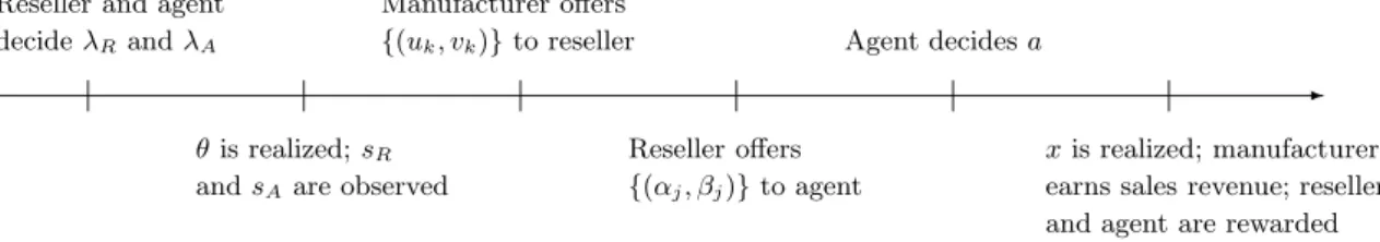
Timing. The sequence of events, as illustrated in Figure 1, is as follows: 1) The reseller’s and
the sales agent’s accuracy λRand λAare publicly observed by everyone. 2) The market condition θ
is realized but observed by no one. The reseller and the sales agent conduct forecasting and observe the demand signals sR and sA, respectively. 3) The manufacturer offers a menu for the reseller to
choose one contract from; 4) Based on the demand signal sR and the chosen contract, the reseller
offers a menu for the sales agent to choose one contract from. In these two stages, if either the reseller or the sales agent rejects the offer, the game ends and every supply chain member receives a null payoff. 5) Based on the signals sR and sA and the chosen contract, the sales agent exerts
sales effort a; 6) The demand quantity x is realized, the sales revenue goes to the manufacturer, and the reseller and the sales agent receive their payments according to the chosen contracts and the realization of x.
-Reseller and agent decide λRand λA
θis realized; sR
and sAare observed
Manufacturer offers {(uk, vk)} to reseller Reseller offers {(αj, βj)} to agent Agent decides a xis realized; manufacturer earns sales revenue; reseller and agent are rewarded Figure 1: Sequence of events.
In the next section, we address our main research questions within the basic framework. We then relax certain assumptions in Section 5 to demonstrate the robustness of the insights we obtain.
4
Analysis
In this section, we first characterize the optimal menus of contracts offered by the manufacturer and the reseller. The impact of the downstream players’ forecasting accuracy on the manufacturer’s profitability and the possibility of interest alignment are then discussed. For ease of exposition, let the type-(j, k) sales agent be the sales agent observing signals sA = j and sR = k and the type-k
4.1 The contract design problems
Suppose that the type-(j, k) sales agent has chosen a contract (αtk, βtk) by reporting sA= t. Let Njk ≡ E[θ|sA= j, sR = k] be the sales agent’s belief on the expected market condition. Then the
profit-maximizing sales agent chooses his sales effort a to solve
Ajk(t)≡ max a≥0 E [ αtk+ βtkx− 1 2a 2 s A= j, sR= k ] = max a≥0 αtk+ βtkNjka− 1 2a 2.
With the optimizer a∗jk(t) = Njkβtk, the resulting expected profit isAjk(t) = αtk +12βtk2 Njk2. Let Ajk ≡ Ajk(j) and a∗jk ≡ a∗jk(j) be the sales agent’s expected profit and effort under truth-telling.
Taking the sales agent’s response into consideration, the type-k reseller designs a compensa-tions scheme{(αF k, βF k), (αU k, βU k)} to maximize her own expected profit. As the reseller observes
the demand signal sR = k, she believes that sA = j with probability Pjk ≡ Pr(sA = j|sR = k).6
Moreover, because the menu should induce the type-(j, k) sales agent to choose (αjk, βjk), we have
E [x|sA= j, sR= k] = Njka∗jk = Njk2 βjk. Suppose the reseller has chosen a contract (ut, vt) by
reporting sR= t, she will then earn ut− αjk+ (vt− βjk)Njk2 βjk in expectation when the sales agent
sees signal sA= j. Therefore, the type-k reseller solves7 Rk(t)≡ max αF kurs., βF k≥0, αU k urs., βU k≥0 ∑ j∈{F,U} Pjk [ ut− αjk+ (vt− βjk)Njk2 βjk ] (1) s.t. AF k ≥ 0, AU k ≥ 0 (2) AF k ≥ AF k(U ), AU k ≥ AU k(F ). (3)
The objective function (1) maximizes the reseller’s expected profit (based on her own belief). The two individual rationality (IR) constraints in (2) guarantee a nonnegative expected payoff for both types of sales agent. The two incentive compatibility (IC) constraints in (3) ensure that both types of sales agent prefer the contract intended for them. Let Rk ≡ Rk(k) be the reseller’s expected
profit under truth-telling. In the following lemma, we characterize the reseller’s optimal menu.
Lemma 1. If the reseller has observed the demand signal sR = k ∈ {G, B} and has chosen the contract (ut, vt), it is optimal for her to offer the sales bonuses
βF k∗ = vt and β∗U k =
PU k
PU k+ PF k(NF k2 /NU k2 − 1)
vt≡ Ykvt,
6N
jk and Pjkcan be explicitly expressed by λA, λR, θH, and θLby applying Bayesian updating. For example, we
have NF G= [θHλAλR+ θL(1− λA)(1− λR)]/[λAλR+ (1− λA)(1− λR)] and PF G= λAλR+ (1− λA)(1− λR) under
the assumption γ = 1
2. These quantities can also be generalized to functions of γ when γ̸= 1 2. 7
to the sales agent. The reseller’s expected profit is Rk(t) = ut+12Zkvt2, where Zk≡ PF kNF k2 +
PU k2 NU k2
PU k + PF k(NF k2 /NU k2 − 1)
= PF kNF k2 + YkPU kNU k2 .
Inside the coefficient Yk, the term NF k2 /NU k2 − 1 captures the influence of the adverse selection
problem in the reseller-agent relationship. While there is no distortion on βF k∗ , β∗U k is downwards distorted if and only if NF k2 /NU k2 − 1 > 0, which happens when λA > 12. In this case, the sales
agent who observes a favorable signal believes that the sales volume will tend to be high. To better differentiate the two types of sales agents, it is in the reseller’s best interest to distort downwards the sales bonus offered to the type-(U, k) sales agent.
Now we consider the manufacturer’s problem in designing the menu{(uG, vG), (uB, vB)}. Once
the manufacturer sees that the contract (uk, vk) is chosen, it knows that the reseller has observed sR= k. In this case, the conditional expectation of sales is
E[x|sR= k] =
∑
j∈{F,U}
PjkNjka∗jk = PF kNF k2 vk+ PU kNU k2 Ykvk= Zkvk, (4)
and the manufacturer’s expected profit is (1− vk)Zkvk− uk. With our assumption γ = 12, simple
derivations show that the manufacturer will see each type of reseller with probability 12. The manufacturer’s contract design problem is thus formulated as
M ≡ max uGurs., vG≥0, uB urs., vB≥0 ∑ k∈{G,B} 1 2 [ (1− vk)Zkvk− uk ] (5) s.t. RG≥ 0, RB ≥ 0, (6) RG≥ RG(B), RB≥ RB(G). (7)
The two IR constraints in (6) guarantee the reseller’s participation while the two IC constraints in (7) ensure truth-telling. The objective function (5) is to maximize the manufacturer’s expected profit. The optimal solution to the manufacturer’s problem is summarized in the following lemma.
Lemma 2. It is optimal for the manufacturer to offer the sales bonuses vG∗ = 1 and vB∗ = ZB ZG to
the reseller. The manufacturer’s expected profit under the optimal contract is M = 14
[ ZG+ Z2 B ZG ] . The reseller receives RB = 0 if she observes a bad signal, RG= 12(ZG− ZB)(ZZBG)2 if she observes a good signal, andR = 12(RG+RB) = 14(ZG− ZB)(ZZB
G)
2 in expectation.
The same as what we have observed in the reseller-agent relationship, the manufacturer also distorts downwards the sales bonus offered to the type-B reseller unless λR = 12 (which implies
ZG= ZB). This eventually lowers the sales effort and introduces inefficiency when delegating to a
type-B reseller. Intuitively, if there is only a single contract, the reseller should always claim that her signal is bad. This is because achieving a high expected sales outcome under a bad signal is more costly and should be compensated more. Therefore, the manufacturer must make (u∗B, vB∗) sufficiently unattractive to the type-G reseller by cutting down the sales bonus vB∗.
Combining the above two lemmas, we have βF G∗ = 1, βU G∗ = YG, βF B∗ = vB∗, and βU B∗ = YBvB∗.
To facilitate the discussions below, we will refer to vB∗ as the upstream distortion factor, which
appears when the reseller observes a bad signal. Similarly, we refer to Yk as the downstream
distortion factor, which is present when the sales agent observes an unfavorable signal. The smaller
vB∗ or Yk is, the larger distortion we have.
Before we move on to discuss the impact of forecasting accuracy in the supply chain, we con-clude this section by discussing the potential inefficiency caused by decentralization. In particular, it is helpful here to compare the equilibrium outcome derived above with the first-best outcome, which can be implemented by the manufacturer who integrates the two downstream players. While it is straightforward that the manufacturer is better off under the first-best scenario, in the lemma below we show that in expectation the sales effort is lower in the decentralized supply chain. In other words, decentralization hurts the entire supply chain.
Lemma 3. The expected sales effort is strictly lower in the decentralized supply chain than in the
integrated supply chain unless λR= λA= 12.
Whether decentralization results in an effort distortion depends on the two downstream play-ers’ accuracy. If both of them are as uninformative as the manufacturer, decentralization is not detrimental. This is because when there is no information asymmetry in the supply chain, inte-grating the supply chain does not generate any informational benefit. Nevertheless, if λR> 12, the
reseller possesses an informational advantage and the upstream distortion emerges as v∗B < 1. In
this case, integrating the reseller eliminates the information asymmetry and reduces inefficiency. Similarly, integrating the sales agent is beneficial if λA > 12. In short, in our model, integration
reduces inefficiency and distortions if and only if there exists information asymmetry in the supply chain.
4.2 Shape of the manufacturer’s expected profit
So far we have characterized the optimal menus offered by the manufacturer and the reseller, the induced effort level, and the resulting expected profits. We now proceed to discuss the impact of the reseller’s forecasting accuracy. The analysis starts from demonstrating the convexity of the manufacturer’s expected profit in the following proposition. Figure 2 illustrates one particular example, in which the manufacturer’s expected profit is nonmonotone: It is first decreasing and then increasing as the reseller improves her forecasting accuracy. Most of the parameter combinations result in the same nonmonotonicity.
0.5 0.6 0.7 0.8 0.9 1 0.11 0.115 0.12 0.125 0.13 0.135 0.14 0.145
The reseller’s accuracy λR
T h e m a n u fa ct u re r’ s ex p ec te d p ro fi t M (θH = 0.7, θL= 0.4, λA= 0.8)
Figure 2: Nonmonotonicity of the manufacturer’s expected profit.
Proposition 1. The manufacturer’s expected profitM is convex on λR∈ [12, 1].
The above proposition as well as our numerical experiments show that typically the manufac-turer’s expected profit decreases in the reseller’s accuracy when the accuracy is low but increases when the accuracy is high. As we explain in detail below, improving the forecasting accuracy cre-ates three different effects in our three-layer supply chain. How the reseller’s accuracy affects the manufacturer’s profitability then depends on the relative importance of these effects.
Improving the reseller’s accuracy first introduces the conventional better-monitoring effect. As the reseller can better estimate the market condition, she can better infer the sales effort and design a more accurate compensation scheme. This will induce the sales agent to exert a higher sales
effort in expectation. To understand this effect, recall that the downstream distortion factor Yk
depends on N2
F k/NU k2 −1 (cf. Lemma 1). As the reseller sees the good and bad signals with the same
probability, the overall effect of adverse selection is captured by12(NF G2 /NU G2 −1)+12(NF B2 /NU B2 −1),
which can be verified to be decreasing in λR. In short, the better-monitoring effect reduces the
lower-level information asymmetry and brings benefits to the supply chain.
However, in the reseller-agent relationship, changing the reseller’s accuracy also modifies the probability for the reseller to see a certain type of sales agent and introduces the belief-altering effect. If the type-k reseller expects to see the type-(F, k) sales agent more likely, it is more important to limit his information rents through a larger downward distortion on β∗U k (i.e., a smaller Yk).
When the reseller observes the bad signal, her belief on the type-(F, B) sales agent is PF B, which
decreases in λR. Therefore, improving the reseller’s accuracy reduces the level of distortion and
improves supply chain performance. However, the opposite happens on the type-G reseller. As
PF G increases in λR, improving her accuracy enlarges the distortion. The overall impact of the
belief-altering effect may thus be either positive or negative.
When the reseller improves her accuracy, the next lemma indicates that the above two effects will eventually be jointly positive, i.e., the downstream distortion factor Yk will go up. This is
because the detriment of aggravating information asymmetry is especially significant when the sales agent only possesses a little informational advantage. In other words, when the reseller’s accuracy is high, mitigating information asymmetry is the most effective and the better-monitoring effect dominates the belief-altering effect, if it is negative.
Lemma 4. For each combination of k ∈ {G, B}, λA ∈ (12, 1], θH, and θL, there exists a unique threshold ¯λR(k, λA, θH, θL)∈ [12, 1) such that Yk is increasing in λR when λR≥ ¯λR(k, λA, θH, θL).
Now we turn to the manufacturer-reseller relationship. Because the manufacturer is always uninformed, improving the reseller’s accuracy unambiguously aggravates the information asymme-try between the manufacturer and reseller. As the reseller’s signal sR becomes more informative,
she is able to earn a larger information rent upon observing a good signal. In order to pay fewer rents, the manufacturer has the incentive to cut down the bonus for the reseller observing the bad signal (note that ZG increases in λR, ZB decreases in λR, and thus vB∗ decreases in λR). This
rent-extraction effect then allows the manufacturer to better differentiate different reseller types and extract more surplus. Nevertheless, it also aggravates the upstream distortion, creates additional efficiency loss, and drives down the the manufacturer’s share of the total profits in expectation.
The shape of the manufacturer’s expected profit, as a function of the reseller’s accuracy, is jointly determined by the better-monitoring, belief-altering, and rent-extraction effects. When the accuracy is low and the information asymmetry between the manufacturer and reseller is small, any accuracy improvement enlarges the manufacturer’s informational disadvantage substantially. In other words, the rent-extraction effect is strong. At the same time, the accuracy improvement only helps the reseller resolve a relatively small part of her informational disadvantage; this suggests that the better-monitoring effect is weak. Therefore, the rent-extraction effect is dominant in the supply chain and the manufacturer’s profit decreases in expectation when the reseller improves her accuracy. On the contrary, if the reseller has already been highly accurate, the information asymmetry in the upper level is already large. The impact of further enlarging the information asymmetry will become relatively insignificant. In other words, the negative rent-extraction effect is marginal. The positive better-monitoring effect, however, is more significant as it may make the lower level close to efficient. The manufacturer’s profitability is thus improved when the reseller further improves her high accuracy.
4.3 Manufacturer-optimal reseller’s accuracy and supply chain structure
As we have established in Proposition 1, the manufacturer’s expected profitM is convex on λR∈
[12, 1]. Therefore, if the manufacturer has the power to choose a reseller to collaborate among a pool
of resellers, it should delegate to either the uninformed reseller with λR= 12 or the precise reseller
with λR= 1. For a reseller to win the business, it is thus crucial to know which accuracy will be
preferred by the manufacturer. Interestingly, because the reseller in our supply chain does nothing but demand forecasting, including the uninformed reseller is equivalent to operating a direct supply chain with only the manufacturer and the sales agent. Therefore, our analysis in this section also allows us to determine whether the direct supply chain outperforms the indirect one.
To facilitate our discussion, we define λ∗R ≡ argmaxλ
R∈[12,1]M as the manufacturer-optimal reseller’s accuracy.8 As we demonstrate in the next proposition, λ∗R is determined by the market condition ratio η and the sales agent’s accuracy λA.
Proposition 2. Let η1 ≈ 1.3954 and η2≈ 2.2695 be the unique greater-than-one roots of η5− η4−
8In general, λ∗
R is a set (of two possible elements 12 and 1) instead of a scalar. However, for ease of exposition,
when λ∗Ris a singleton, we will use λ∗R= z instead of the more rigorous expression λ∗R={z}. Throughout the paper,
2η2+ η =−1 and η4− 2η3− η2 =−2, respectively. Then λR∗ = 12 if η < η1 and λ∗R= 1 if η > η2. For intermediate values of η ∈ [η1, η2], there exists a unique ¯λA(η) ∈ [12, 1] such that λ∗R = 12 if λA< ¯λA(η), λ∗R= 1 if λA> ¯λA(η), and λ∗R={12, 1} if λA= ¯λA(η).
We visualize the above proposition in Figure 3, in which ¯λA(η) is illustrated by the curve as a
function of η on the interval [η1, η2]. λ∗R is different in the two regions separated by the curve. The
first determinant of λ∗R is the market condition ratio η ≡ θH
θL. Recall that θH and θL are the two possible realizations of θ, the random market condition. When η < η1, the difference between θH
and θL is small, and naturally the benefit of distinguishing the two realizations is only marginal:
A wrong estimate does not deviate from the actual state too much. Therefore, the strength of the precise reseller is limited and the uninformed reseller is preferred. When η > η2, the result is
opposite and the precise reseller is preferred. This is because distinguishing the two quite different realizations now becomes so valuable that the precise reseller helps the manufacturer a lot.
The market condition ratio η
T h e sa le s a g e n t’ s a cc u ra cy λA 1 1.2 1.4 1.6 1.8 2 2.2 2.4 0.5 0.6 0.7 0.8 0.9 1 λ∗ R= 1 2 λ∗ R= 1 η1≈ 1.3954 η2≈ 2.2695
Figure 3: Manufacturer-optimal reseller’s accuracy.
The problem is more interesting when η is moderate, i.e., between the two cutoffs. Because the rent-extraction effect appears in the manufacturer-reseller relationship, it harms the manufacturer in the same way regardless of the sales agent’s accuracy. On the contrary, the amount of benefits brought by the better-monitoring effect critically depends on how accurate the sales agent is. When the sales agent is highly accurate, the manufacturer must find a way to mitigate the information asymmetry. This is why it should include the precise reseller for indirect monitoring. As in Figure
3 the range of η for λ∗R= 1 enlarges when λA increases, the above arguments is verified.
4.4 Reseller-optimal reseller’s accuracy and interest alignment
In some situations, the manufacturer has no choice but to collaborate with the reseller, and it is the reseller’s discretion to choose her forecasting accuracy. In this case, it is important for the manufacturer to ask whether these two players’ interests are aligned with each other, i.e., whether the manufacturer-optimal reseller’s accuracy is also reseller-optimal and will be selected by the reseller voluntarily. The current practice for the manufacturer to affect the reseller’s accuracy decision is meaningful only if the answer is no.
When the reseller selects her accuracy to maximize her own expected profit R, let λ′R ≡
argmaxλ
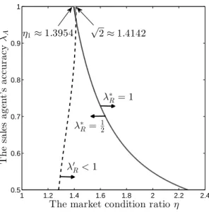
R∈[12,1]R be the reseller-optimal reseller’s accuracy. Our next proposition says that interest alignment between the two upstream players, i.e., λ′R = λ∗R, is possible only when η is moderate and λA is large. Moreover, if it happens, it must be that λR= 1.
Proposition 3. λ′R= λ∗R only if η ∈ [η1, √
2] and λA ≥ max{¯λA(η), ˜λA(η)}, where η1 and ¯λA(η) are defined in Proposition 2 and ˜λA(η) ≡
2η3−3η−√−η(2η2−3)(η2−2)
2η3+η2−3η−η for η ∈ [η1,
√
2]. Whenever
λ′R= λ∗R, we have λ′R= λ∗R= 1.
Figure 4 provides an illustration for Proposition 3. The solid curve representing ¯λA(η) comes
from Figure 3, which separates the two regions having different λ∗R. The dashed curve depicts ˜λA(η)
defined in Proposition 3. To the right of the dashed curve, we have λ′R< 1. The shaded area above
both curves is the only region that the supply chain may be coordinated.9
We explain the result in two steps. First, because the reseller in our model can do nothing but demand forecasting, the ability of alleviating information asymmetry is her only instrument to earn profits. In fact, as we demonstrate in the proof, the reseller is expected to earn zero profit if λR= 12. Therefore, the reseller always prefers to be at least partially informed. It then follows
that there is always interest misalignment when the manufacturer prefers the uninformed reseller. In the region where the uninformed reseller is preferred (to the left of the solid curve), the interests are never aligned. The above intuition also explains why λR= 1 is required for interest alignment.
9Inside the shaded region, indeed we observe supply chain coordination in some cases. For example, when η = 1.4
1 1.2 1.4 1.6 1.8 2 2.2 2.4 0.5 0.6 0.7 0.8 0.9 1
The market condition ratio η
T h e sa le s a g en t’ s a cc u ra cy λA λ′ R< 1 λ∗ R= 1 λ∗ R= 12 √ 2 ≈ 1.4142 η1≈ 1.3954
Figure 4: Interest alignment between manufacturer and reseller.
Now consider the dashed curve ˜λA(η). As shown in the proof of this proposition, we have λ′R < 1 in the region that is to the right of the dashed curve. To understand why a large value
of η discourages the reseller from being precise, note that the better-monitoring effect drives up the sales agent’s sales bonus and the rent-extraction effect lowers the reseller’s sales bonus. As both effects are detrimental from the reseller’s perspective, the reseller faces a trade-off between creating a larger pie and owning a smaller share of the pie. When η is sufficiently high, the reseller’s accuracy is important in tackling demand uncertainty. The two effects are thus too strong and the reseller will avoid high accuracy that leaves her a too small share.
When η is moderate, we also need to take the sales agent’s accuracy λAinto account. Consider
the case when λA decreases. While the manufacturer-reseller relationship is unchanged and the
rent-extraction effect retains its impacts, the reseller-agent relationship becomes different and the better-monitoring effect becomes weaker. The benefit of enlarging the total pie is thus reduced a lot. However, the cost of having a smaller share, though it is also reduced, remains substantial as the rent-extraction effect is still significant. It then follows that the reseller will not improve her accuracy to a too high level. This explains why λ′R< 1 when λA is small.
Collectively, as we may observe in Figure 4, Proposition 3 implies that usually there is interest misalignment in the upper level of our supply chain. When the manufacturer prefers the uninformed reseller (λ∗R= 12), the interests cannot be aligned; when the reseller prefers herself not to be precise
(λ′R< 1), the interests are also not aligned. Nevertheless, in our setting the two upstream players’
interests may still be automatically aligned without adopting any coordination mechanism. It should be noted that the interest alignment critically depends on the assumption that there is no cost for enhancing accuracy. As long as the cost of achieving λR = 1 is higher than 1 4(θ 2 H − θL2)( θL θH)
2, the precise reseller’s expected profit derived in Lemma 2, the reseller will not
prefer to be precise and thus interest alignment is impossible. If the manufacturer prefers a precise reseller, some mechanisms (e.g., subsidization) will be required for aligning the interests.
4.5 Impact of the sales agent’s accuracy
Now we also accommodate the sales agent’s accuracy decision. Our first result, which is in line with Proposition 1, establishes the convexity of expected profits with respect to the sales agent’s accuracy.
Proposition 4. The manufacturer’s expected profitM is convex on λA∈ [12, 1].
Once the sales agent improves his accuracy, he can exert efforts in response to the market
condition more accurately and make the supply chain more efficient. However, improving his
accuracy also increases the information asymmetry in the reseller-agent relationship and hurts the manufacturer. Therefore, the manufacturer’s expected profit is also convex and typically first decreasing and then increasing in the sales agent’s accuracy.
Proposition 4 is helpful for us to find the manufacturer-optimal accuracy mix, i.e., the combi-nation of the reseller’s and the sales agent’s accuracy that maximizes the manufacturer’s expected profit. With the convexity of M with respect to λA, it is immediate that λA must be either 12
or 1 in any manufacturer-optimal accuracy mix. However, while improving the reseller’s accuracy introduces conflicting effects, improving the sales agent’s accuracy results in only negative effects: The information asymmetry in the manufacturer-reseller relationship remains unchanged but that in the reseller-agent relationship is aggravated. It is thus unsurprising that the manufacturer always prefers the sales agent to be uninformed, as indicated in the following proposition.
Proposition 5. For all η, if λA = 1 in a manufacturer-optimal accuracy mix (λR, λA), fixing λR but changing λA to 12 is also manufacturer-optimal. Moreover, if η < η2, which is defined in Proposition 2, we have λA= 12 in any manufacturer-optimal accuracy mix.
Proposition 5 has an important implication on interest alignment in the supply chain. Suppose now both the reseller and the sales agent choose their accuracy to maximize their own expected
profits. Proposition 3 has shown that the manufacturer’s interest cannot be aligned with the
reseller’s for η ≥ η2. For η < η2, to maximize the manufacturer’s expected profit, Proposition 5
requires the sales agent to be uninformed, which is never preferred by the sales agent because this leaves himself a zero expected profit. We thus establish the following corollary.
Corollary 1. If both the reseller and sales agent can choose their forecasting accuracy, the
manu-facturer’s interest can never be aligned with the two downstream players simultaneously.
5
Extensions
In this section, we extend our basic model to investigate the robustness of our findings. Specifically, we consider scenarios in which the sales outcome is continuous, improving forecasting accuracy is not free, the sales agent is protected by limited liability, and the distribution of the market condition is general. As we show in the sequel, the main insights established in Section 4 remain valid under these new settings. In addition, enriching our model generates new findings and makes our results applicable in a more general environment.
5.1 Continuous sales outcome
Our results in Section 4 are established based on the assumption that the sales outcome x is binary. In the basic model, the probability for the sales outcome to be high depends on the market condition
θ and the sales effort a in a multiplicative form, i.e., Pr(x = 1|θ, a) = θa. Under this assumption,
when the sales agent exerts a higher effort, he is uncertain whether the sales quantity will really increase even if he is precise and can observe the market condition. The demand uncertainty makes exerting a high effort risky and constitutes the source of all informational issues in our supply chain. Therefore, it is natural to ask whether we may extend our basic model by removing the binary assumption and model the demand uncertainty in a different way while maintaining our main findings.
To show that our results are not prone to the binary assumption, we adopt a continuous demand model and assume a new format of the sales outcome x = θa. To preserve the way to conduct forecasting, the market condition θ ∈ {θL, θH} is still assumed to be binary and takes
either realization with probability 12. It then follows that the reseller and sales agent forecast in the same way. However, now the sales agent may directly affect the sales outcome with his sales effort. When he increases his effort level by 1, the sales agent is certain that the sales volume will increase by either θLor θH. Moreover, in the extreme case that either the reseller or the sales agent
is precise (i.e., can observe the realization of the market condition), demand uncertainty disappears from the sales agent’s perspective. Also the parameters θL, θH, and the effort decision a are all not
limited to be between 0 and 1. The examination of our analysis and results will help us evaluate the applicability of our findings.
As the sales outcome is no longer binary, the contract forms also need to be redefined. As moral hazard problems with a continuous demand is known to be intractable, we assume that the reseller offers linear contracts, i.e., two-part tariffs, for the sales agent to self-select. In such a scenario, a contract consists of a fixed payment and a commission rate such that the sales agent’s earning is the fixed payment plus the commission rate times the sales outcome. The contractual agreements between the manufacturer and the reseller are defined in the same format.
Under the new model setting, the sales agent makes his effort decision in the same way by balancing his cost of effort exertion with the expected payoff from the increased sales volume. Interestingly, we find that the type-(j, k) sales agent’s equilibrium effort level can still be expressed as Njkβjk, where Njk =E[θ|sA= j, sR= k] is the expected market condition given his information
and βjk is the commission rate chosen by him. In other words, even though the underlying meanings
of Njk and βjk become different from those in the basic model, they still decide the sales agent’s
effort choice in the same way. It then follows that the reseller and manufacturer design their contracts as in Section 4. Therefore, none of our insights obtained in the previous section will
change under the continuous demand model.10
5.2 Limited liability of the sales agent
Suppose the sales agent is now protected by limited liability and cannot afford a large payment to the reseller. More precisely, in the reseller’s contract design problem, we now include the limited
liability constraints αG ≥ −C and αB ≥ −C, where C ∈ [0, ∞) is the highest amount of fixed
payment that the sales agent can afford to pay to the reseller. We will first focus on the extreme
10
Alternatively, we may adopt the additive form x = θ + a, which is not possible under the original binary setting. Nevertheless, we do not find any new insight and thus the derivations are omitted.
case in which the sales agent cannot pay any positive fixed payment to the reseller, i.e., C = 0, and discuss the general case with C > 0 at the end of this section. The next proposition shows that, when C = 0, the limited liability does not change the shape of the manufacturer’s expected profit but has a significant impact on the manufacturer-optimal reseller’s accuracy.
Proposition 6. When the sales agent cannot pay any fixed payment, the reseller offers a single
contract to the sales agent. Moreover, the manufacturer’s expected profit is convex in the reseller’s accuracy and is strictly higher with the uninformed reseller than with the precise one.
With the presence of limited liability, first we find that the reseller offers a single contract to both types of sales agents. This is because the limited liability is so strict that no menu can successfully distinguish the two types of sales agents. It is also shown that the manufacturer’s expected profit is still convex in the reseller’s accuracy. More interestingly, the uninformed reseller now strictly dominates the precise reseller from the manufacturer’s perspectives. In the presence of limited liability, the negative rent-extraction effect remains in the manufacturer-reseller relationship. For the reseller-agent relationship, however, because the reseller cannot distinguish the two types of the sales agent, the positive better-monitoring effect no longer exists. Though the sales agent can still exert efforts more efficiently when the reseller improves her accuracy, the lack of the positive better monitoring effect greatly reduces the benefit of improving the reseller’s accuracy. The rent-extraction effect then becomes dominant and the uninformed reseller is strictly preferred. In short, because it is impossible to mitigate the information asymmetry in the reseller-agent relationship due to the sales agent’s limited liability, it is optimal to eliminate the information asymmetry in the manufacturer-reseller relationship by keeping the reseller uninformed.
When C > 0, how the degree of limited liability affects the supply chain depends on the two optimal fixed payments charged by the reseller defined in Lemma 1, α∗F and αU∗. When−C ≥ α∗U, the fixed payments offered to the sales agent change from 0 to −C but the sales bonuses are still the same as if C = 0. All our results established in this section hold. When −C ∈ (α∗F, α∗U), the reseller offers a menu of contracts and brings the better-monitoring and belief-altering effects back. However, if C is sufficiently close to α∗U, the two effects will only be marginal and the uninformed reseller still dominates the precise one. The precise reseller may generate a higher expected profit only if −C is close enough to α∗F. Finally, when −C ≤ α∗F, the optimal menu without limited liability is acceptable by the sales agent and all the results in Section 4 hold. In this case, all players interact as if there is no limited liability.
5.3 General levels of pessimism
So far we have restricted our analysis to the case that the level of pessimism γ≡ Pr(θ = θL) = 12. We
now remove this assumption and allow γ to be any number within the interval (0, 1). The procedure of deriving the equilibrium behaviors when γ ̸= 12 is almost identical to that when γ = 12. As the only modification is to generalize the quantities Njk, Pjk, Zk, and the probability for the reseller
to see the good signal to be functions of γ, we omit the details here. Unfortunately, even though the closed-form expressions of optimal contracts and efforts can still be derived, the generalization of γ greatly complicates our three-layer supply chain and prevents us from obtaining clear-cut analytical results in terms of the manufacturer’s profitability and preferences. Therefore, we resort to numerical experiments to generate insights. Our first observation is in line with Proposition 1 and characterizes how the reseller’s accuracy affects the manufacturer’s expected profit.
Observation 1. For any value of γ, the manufacturer’s expected profitM is either first decreasing
and then increasing or monotonically decreasing in the reseller’s accuracy λR∈ [12, 1]. In particular, M tends to be nonmonotone when γ is low but monotonically decreasing when γ is high.
Though generalizing the level of pessimism destroys the convexity in general, it qualitatively preserves the relationship between the manufacturer’s expected profit and the reseller’s accuracy. This is because those conflicting effects still exist under any value of γ and thus the shape of the manufacturer’s profitability remains similar. More interestingly, we find that the value of γ plays a role in determining the shape of the manufacturer’s expected profit. For each curve in Figure 5, the manufacturer’s expected profit is monotonically decreasing in λR at the left-hand
side but nonmonotone at the right-hand side. When γ decreases, the right-hand side enlarges and the manufacturer’s expected profit is more likely to be increasing in λR when λR is large. This is
because if the reseller becomes more accurate under a low level of pessimism (small γ), it is more likely for her to observe the good signal more often, to offer a more generous contract, and to induce a higher sales effort. The manufacturer thus benefits from such an improvement. On the contrary, increasing γ enlarges the left-hand side makes the manufacturer’s expected profit more likely to be decreasing in λR when λR is large. This is due to the fact that under a high level of pessimism
(large γ), being more accurate makes the reseller more pessimistic and drives the expected effort level down. Consequently, the manufacturer earns less in expectation.
Our next step is to investigate how different values of γ affect the manufacturer-optimal re-seller’s accuracy λ∗R. Recall that in Proposition 2 and Figure 3 we characterize and visualize the
1 1.2 1.4 1.6 1.8 0.5 0.6 0.7 0.8 0.9 1
The market condition ratio η
T h e sa le s a g e n t’ s a c cu ra c y λA γ = 0.4 γ = 0.2 γ = 0.5 γ = 0.6 γ = 0.8
Figure 5: Monotonicity of the manufacturer’s expected profit with various levels of pessimism.
two-dimensional cutoff structure when γ = 12. As we summarize in the next observation, the same structure still applies to other values of γ. This observation is visualized in Figure 6, where we depict several cutoff curves under various values of γ. For each curve, the manufacturer-optimal reseller’s accuracy is λ∗R = 12 at the left-hand side and λ∗R = 1 at the right-hand side. It is clear that all these curves have similar shapes and the insight we obtained for the special case γ = 12 is still valid.
Observation 2. For any γ ∈ (0, 1), the manufacturer’s expected profit M is maximized at λ∗R= 12
(respectively, λ∗R= 1) if η and λA are both small (respectively, large) enough. Moreover, it is more likely that λ∗R= 12 (respectively, λ∗R= 1) when γ increases (respectively, decreases).
The second part of Observation 2 delivers more messages to us regarding the impact of the level of pessimism γ on the manufacturer-optimal reseller’s accuracy λ∗R. As γ increases, improving the reseller’s accuracy makes the reseller more pessimistic. The manufacturer thus prefers the uninformed reseller more. Decreasing γ introduces the opposite effect and makes the manufacturer prefer the precise reseller more. Interestingly, even if γ is extremely close to 0, it is still possible that delegating to an uninformed reseller is optimal for the manufacturer. The following proposition provides an analytical support.
The market condition ratio η T h e sa le s a g e n t’ s a c cu ra c y λA 1 1.4 1.8 2.2 2.6 3 0.5 0.6 0.7 0.8 0.9 1 γ = 0.6 γ = 0.8 γ = 0.5 γ = 0.4 γ = 0.2
Figure 6: Manufacturer-optimal reseller’s accuracy with various levels of pessimism.
that delegating to the uninformed reseller uniquely maximizes the manufacturer’s expected profit if λA< ´λA(γ, η).
6
Conclusion
In this paper, we consider a three-layer supply chain with a manufacturer, a reseller, and a sales agent. While the manufacturer is uninformed about the realization of the random market condition, both the reseller and the sales agent can conduct demand forecasting to estimate the realized market condition. We show that the manufacturer’s profitability is hurt when the reseller or the sales agent improves her/his low accuracy. When the accuracy is high, however, an improvement may allow the manufacturer to earn more in expectation. From the manufacturer’s perspective, when the market demand is only slightly volatile and the sales agent is not accurate, the uninformed reseller is preferred; when the demand is highly volatile and the sales agent is pretty accurate, delegating to the precise reseller is optimal. We also find that the manufacturer’s interest may be aligned with the reseller’s when only the reseller can choose her accuracy. However, this alignment is never possible when both downstream players have the discretion to choose their accuracy.
Our study certainly has its limitations. In this study, we exclude the possibility for the
is pervasive in practice, there are also situations where the sales agent is hired or can be directly compensated by the manufacturer (for more details about this situation, see, e.g., [14]). New insights may be found under this alternative setting. We also assume that the forecasting accuracy is public to every supply chain member. Removing this assumption will introduce the necessity of a two-stage screening process (one for the accuracy and the other for the signal) and may change some of our results. Finally, a promising direction is regarding the interest alignment issue we point out in this study. When the downstream players are allowed to choose their own accuracy, it is highly possible that the equilibrium accuracy mix will be manufacturer-suboptimal. Whether there exists any mechanism to align the interests remains open and calls for further investigation.
Appendix
Proof of Lemma 1. First, we can apply AF k ≥ AF k(U ), NF k2 ≥ NU k2 , and AU k ≥ 0 to show
that AF k ≥ 0 is redundant. If we ignore the constraint AU k ≥ AU k(F ), the remaining two
constraints will be binding at the optimal solution. Therefore, we can replace αF and αU by
αF = 12βU2(NF k2 − NU k2 )−12β 2
FNF k2 and αU = −12βUNU k2 in the objective function. The problem
then reduces to Rk(t) = max βF≥0,βU≥0 PF k [ 1 2N 2 F kβF2 − 1 2(N 2 F k− NU k2 )βU2 + NF k2 (vt− βF)βF ] +PU k [ 1 2N 2 U kβU2 + NU k2 (vt− βU)βU ] , (8)
which is solved by βF∗ = vt and β∗U =
PU kNU k2
PU kNU k2 +PF k(NF k2 −NU k2 )
vt through the first-order condition.
Verifying the constriantAU k ≥ AU k(F ) is trivial and omitted. The reseller’s expected profitRk(t)
can be found by plugging βF∗ and βU∗ into (8).
Proof of Lemma 2. First, we can applyRG ≥ RG(B), ZG≥ ZB, andRB≥ 0 to show that RG≥
0 is redundant. If we ignore the constraint RB ≥ RB(G), the remaining two constraints will be
binding at the optimal solution. Therefore, we can replace uGand uBby uG= v2 B 2 (ZG−ZB)− v2 G 2 ZG and uB=− v2 B
2 ZB in the objective function. The problem then reduces to
M = max vG≥0,vB≥0 { 1 2ZGv 2 G− 1 2(ZG− ZB)v 2 B+ ZG(1− vG)vG+ 1 2ZBv 2 B+ ZB(1− vB)vB } , (9)
which is solved by vG∗ = 1 and v∗B= ZB