數位影像穩定技術及其應用

國

立

交

通

大

學

電控工程研究所

博

士

論

文

數位影像穩定技術及其應用

Digital Image Stabilization Technique and its Applications

研 究 生：徐聖哲

指導教授：林進燈 教授

數位影像穩定技術及其應用

Digital Image Stabilization Technique and its Applications

研 究 生：徐聖哲 Student：Sheng-Che Hsu

指導教授：林進燈博士 Advisor：Dr. Chin-Teng Lin

國 立 交 通 大 學

電控工程研究所

博 士 論 文

A Dissertation

Submitted to Institute of Electrical Control Engineering College of Electrical and Computer Engineering

National Chiao Tung University in partial Fulfillment of the Requirements

for the Degree of Doctor

in

Electrical Control Engineering June 2010

Hsinchu, Taiwan, Republic of China

數

位

影

像

穩

定

技

術

及

其

應

用

學生：徐聖哲指導

教授：林進燈教授

國立交通大學電控工程研究所 博士班

摘

要

本論文為提出數位影像穩定技術研究成果及其應用，本文中提出如何在手持式、車 用或固定式監視攝影機，因人為不可預期的抖動、車輛行駛巔岥、方向盤轉動的效應或 風力、外力等的影響而造成影像的抖動，以數位影像處理的方式去除不必要的抖動而保 留必要的移動。數位影像穩定技術主要可分為兩部份：(1)如何從影像序列中有效率地估 算出準確、可靠的全域移動向量；(2)如何從所取得的移動向量在邊界的限制下補償出一 平滑的影像運動軌跡。 本文在移動向量估測上提出倒三角方法以尋找區域移動向量、最佳化代表點選擇以 降低尋找移動向量的計算量、產生精煉型移動向量以應用在乏特徵的狀況仍可估算全域 移動向量、另提出天際線的檢測方法與以背景為基礎的對等演算法以求得較可靠的全域 移動向量。 本文在移動向量補償上提出移動軌跡的繪製與平滑指標的計算以驗證所提出移動 向量補償方法改善數位影像穩定的定量分析，同時在補償方法中提出在回路中加上一內 部回授積分器以改善鏡頭在定速移動時造成補償效果不良的問題。最後則以模糊推論的 機制，以兩種不同的方法透過模糊推論，選擇較佳的補償方式，以適應數位影像防振在 各種情況的應用。 經實驗的結果，本文所提出的方法可適用在不同狀況的影像序列如乏特徵、重複圖 樣、大移動物件及大區域低對比的影像狀況，而能估算出準確的全域移動向量。在移動 向量補償上則解決在定速移動下所造成補償效果降低的問題，並以模糊推論整合方式有 效地改善補償向量的補償效果，從平滑指標與移動軌跡圖上均可驗證本文所提出的方法 有效地改善數位影像穩定的效能。

Digital Image Stabilization Technique and its Applications

Student：Sheng-Che Hsu Advisors：Dr. Chin-Teng Lin

Institute of Electrical Control Engineering

National Chiao Tung University

Abstract

In this dissertation, a digital image stabilization (DIS) technique and its applications are proposed as a way to remove the unwanted shaking phenomena in the image sequences captured by hand-held, in-car or fixed-type surveillance camcorders, without being affected by moving objects in the image sequence or by the intentional panning motion of the camera. DIS contains two major parts: (1) How to estimate an efficient, precise, and reliable global motion vector. (2) How to use the existing GMV to compensate for a smooth motion trajectory within the window shifting allowance boundary.

For motion estimation (ME), an inverse triangular method is proposed to look for the local motion vector (LMV). An optimization of the representative points is proposed to reduce computation complexity, and a refined motion vector is proposed to apply to any ill-conditions of the GMV estimation. Skyline detection for in-car applications and background based peer to peer evaluation are proposed to enforce the reliability of the GMV estimation as well.

For motion compensation (MC), a plot of the motion trajectory and a smoothness index evaluation are proposed to quantitatively verify the analysis that shows the improvement of the MC. An inner feedback-loop integrator has been applied to the MC to improve image stabilization during the camera’s panning motion. Finally, Fuzzy inference digital image stabilization (FIDIS) is proposed to adaptively determine better motion compensation methods through the use of two different MCs.

Experimental results show that the proposed methods of this dissertation adapt to different conditions of image sequencing, such as a lack of features, repeated patterns, large moving objects and large low-contrast areas in the image and that they can also estimate the GMV precisely as well. The degradation of image stabilization during the panning motion is solved by adding an inner feedback-loop integrator. The proposed FIDIS also shows effective

improvements in different conditions of image sequence through the evaluations of the smoothness index and the motion trajectory.

Acknowledgement

首先感謝指導教授林進燈教務長多年來的指導。無論在專業上或生活上的指導與照 顧，都使我受益良多。林進燈教授在研究上的精神是我學習最佳的榜樣，其待人誠懇平 易近人及樂於助人的特質更是讓我在進修博士班十年的歲月中最大的鼓勵。對於本論文 的完成，林教授給與我很大的鼓勵與支持，再次由衷的感謝。 在家人方面，謝謝年邁的父親，從您過去以身作則堅持與毅力的表現，在在影響我 對進入博士班深造與進修的持續。謝謝我的妻子巽俐與兩位可愛的女兒蕙心、蕙薰，多 年來因為學業與工作的關係使得陪你們的時間相對減少，你們對我的期待與包容成為我 可以完成這樣的一個理想，如果沒有你們的支持與鼓勵，那將是一件不可能的任務，謝 謝！我愛你們。 最後謝謝論文口試委員郭耀煌教授、蔡文祥講座教授、陳永耀教授、陳永昌教授、 張志永教授、陳永平教授、蒲鶴章博士，由於您們熱心的指導與建議使論文更加完整， 在此致上最高的敬意。

Table of Contents

Abstract (In Chinese)...i

Abstract (In English) ...ii

Acknowledgement...iv

Table of Contents...v

List of Tables ...vii

List of Figures...viii

1. Introduction ...1

1.1. Motivation ...1

1.2. Related Works Review ...1

1.3. Overview of This Dissertation...4

2. Motion Estimation ...6

2.1. Introduction ...6

2.2. Motion Estimation ...10

2.2.1. Motion Estimation Architecture ...10

2.2.2. RPM and Local Motion Estimation... 11

2.2.3. Irregular Condition Detection...12

2.2.4. Determination of Representative Point Amount...19

2.2.5. Optimization of Representative Points...19

2.2.6. Generation of Refined Motion Vector ...21

2.2.7. Global Motion Estimation ...22

2.2.7.1. Background Based Peer to Peer Evaluation ...23

2.2.7.2. Skyline Detection ...24

2.3. Summary...27

3. Motion Compensation ...28

3.1. Introduction ...28

3.2. Compensating Motion Estimation...29

3.2.2. Quantitative Evaluation ...30

3.2.3. Compensation with Inner Feedback-Loop Integrator...30

3.2.4. Fuzzy Inference Digital Image Stabilization (FIDIS) ...32

3.3. Summary...37

4. Experimental Results...38

4.1. Experiment Results of ORP...38

4.2. Performance of Compensation with Inner Feedback-Loop Integrator...41

4.3. Experimental Results of FIDIS ...48

5. Conclusions ...52

Bibliography ...54

Author’s Publication List...58

List of Tables

Table 4.1. RMSE comparisons of RPM_FUZZY and the proposed method with respect to four real video sequences. ...43 Table 4.2. SI comparisons of three CMV generation methods...43 Table 4.3. The parameters applied to CMV generation with different equations..47 Table 4.4. SI comparisons of two different CMV generation methods with respect

to four different GMV sets...47 Table 4.5. SI comparisons of three methods with respect to four GMV sets ...51

List of Figures

Fig. 1.2. Schematic overview of the digital image stabilization developing

techniques...4 Fig. 2.1. System architecture of the proposed digital image stabilization technique.

...10 Fig. 2.2. Block diagram of LMVs and RMV estimation...10 Fig. 2.3. Division of image for local motion vector estimation. ... 11 Fig. 2.4. Various correlation curves corresponding to image sequences with

different conditions (I). (a) A normal condition. (b) Lacks feature in vertical direction (book). (c) Repeated patterns (office). (d) Moving object (bear). (e) Large low-contrast area (white wall). Video images are captured by camcorder in daily life scene...16 Fig. 2.5. Various correlation curves corresponding to image sequences with

different conditions (III). (a) A normal condition. (b) Lacks feature in horizontal direction. (gate) (c) Repeated patterns (brick). (e) Moving object (motorcycle). (f) Large low-contrast area (sky).Video images are captured by in-car video camera in outside scene...17 Fig. 2.6. Examples of minimum projections of correlation curve from x and y

directions in four regions. (a) Regular image sequence. (b) Ill-conditioned image sequence. ...18 Fig. 2.7. Illustration of the proposed inverse triangle method. ...18 Fig. 2.8. The experimental result of calculating the cost level (that is an index of

reliability defined in Eq. (2.13)) by using different number of

representative points...19 Fig. 2.9. The illustration of optimal representative point selection method. (a) The

original image. (b) The traditional representative points. (c) The optimal representative points. (d) The optimal representative points after neglecting insignificant points. ...21

Fig. 2.10. Areas for background detection and evaluation...24

Fig. 2.11. Areas for the background-based evaluation adapted by the detected skyline. ...26

Fig. 2.12. Skyline detection algorithm is to combine RPM correlation evaluation, minimum projection and inverse triangle method...26

Fig. 2.13. Skyline detection applies on the in-car video sequence taken from highway. ...26

Fig. 3.1. Trajectories of motion generated by original global motion vectors and compensated global motion vectors. The compensated motion trajectory generation method in (3.1) ...29

Fig. 3.2. The original and the compensated motion trajectories. (a) CMV generation method in (3.1) with clipper in (3.2). (b)Proposed method in (3.3)...32

Fig. 3.3. Block diagram of the proposed CMV generation method. ...32

Fig. 3.4. Overshoot in low frequency image panning back and forth. ...33

Fig. 3.5. Architecture of fuzzy inference applied to digital image stabilization. ...33

Fig. 3.6. Architecture of fuzzy inference system...34

Fig. 3.7. Architecture of internal fuzzy inference...35

Fig. 3.8. Membership functions of inputs (a)ΔSI n( ); (b)Δd n( )...35

Fig. 3.9. Membership function of output...36

Fig. 4.1. The illustration of optimal representative point selection method. (a) The original image. (b) The traditional representative points. (c) The optimal representative points. (d) The optimal representative points after neglecting insignificant points. ...39

Fig. 4.2. The local motion vector of each region. Only region 4 appears the local motion due to the bear moving from the right to the left side...40

Fig. 4.3. The bear is moving from the left to the right side and the background is moved from the left-bottom to the right-up. The motion vector in regions 1, 2 and 3 contain the global motion. Region 4 contains the combination of the local and global motions. ...40

Fig. 4.4. The plots of original and compensated motion trajectories. (a) In x axis (b) In y axis. ...40 Fig. 4.5. Performance comparison of three different CMV generation methods

with clipper in Eq. (3.5). (c) The proposed method in Eq. (3.6)...44 Fig. 4.6. Comparisons of original and compensated motion trajectories by two

different CMV generation methods (with and without integrator) with respect to (a) GMV set #1, (b) GMV set #2, (c) GMV set #3, (d) GMV set #4...46 Fig. 4.7. Comparisons of original and compensated motion trajectories by three

methods, MC#1, MC#2 and FIDSI with respect to GMV#1. ...49 Fig. 4.8. Comparisons of original and compensated motion trajectories by three

methods, MC#1, MC#2 and FIDSI with respect to GMV#2. ...49 Fig. 4.9. Comparisons of original and compensated motion trajectories by three

methods, MC#1, MC#2 and FIDSI with respect to GMV#3. ...50 Fig. 4.10. FIDIS operation illustrated by short term smoothness SI n and fuzzy ( )

1. Introduction

1.1. Motivation

Digital video sequences acquired by image captured devices are usually affected by undesired motions which can be classified into several aspects. The image captured by compact and lightweight video cameras, i.e. hand held devices, are usually affected by unstable camera holding or moving platform. The image captured by in-car video cameras are usually affected by a bumpy ride or by the steering of the driver. The image captured by video surveillance systems are usually affected by wind blowing, bird jumping or earthquake. The unwanted positional fluctuations of the video sequence will affect the visual quality and impede the subsequent processes for various applications such as motion coding, video compression, feature tracking, etc. The challenges of a digital image stabilization system (DIS) are: how to compensate for the unwanted shaking of the devices without being affected by large moving objects, ill conditions in the image, and the panning motion of the camera. In this dissertation, the related techniques of DIS will be proposed to tackle these challenges.

1.2. Related Works Review

The image stabilization systems can be classified into three major types: (1) the electronic image stabilizers (EIS) [1]; (2) the optical image stabilizers (OIS) [2]; (3) the digital image stabilizers (DIS) [5]. The EIS stabilizes the image sequence by employing motion sensors to detect the camera movement for compensation. The OIS employs a prism assembly that moves opposite the shaking of the camera for stabilization. Because both EIS and OIS are hardware dependant, the applications are restricted to device built-in on-line process. The (DIS) is the process of removing the undesired motion effects to generate a compensated image sequence by using digital image processing techniques without any mechanical devices such as gyro sensors or fluid prism [4]. The major advantages of DIS are: (1) no restriction of on/off-line applications, (2) suitable for miniature hardware

implementation (since the mechanical device is not required for compensation) [5]. The DIS can be performed either as post-processing after the video sequence was acquired, or in real-time during the acquisition process, depending on the applications. Archive films with undesired shaking effects require post-processing for the video sequences, while camcorders require a real-time compensation process.

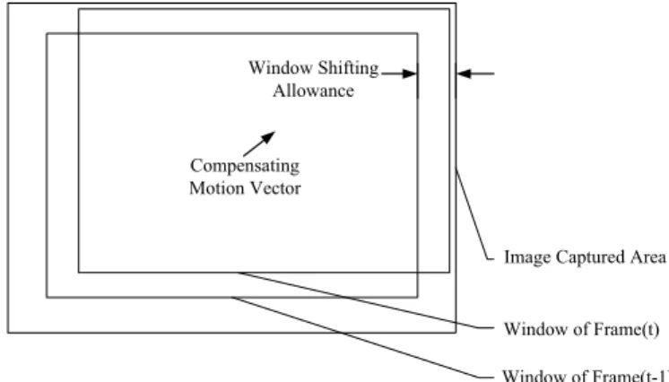
The DIS system is generally composed of two processing units. One is the motion estimation unit and the other is the motion compensation unit. The purpose of motion estimation unit is to estimate the reliable camera global movement through three processing steps on the acquired image sequence. (1) evaluation of local motion vectors (LMVs) is the first step of the process; (2) detection of unreliable motion vector components is the next step. (3) determination of the global motion vector (GMV). Following the motion estimation, the motion compensation unit generates the compensating motion vector and shifts the current picking window according to the compensating motion vector to obtain a smoother image sequence. Fig. 1.1 shows the motion compensation schematics. The window of frame( 1)t− is the previous compensated image. The compensating motion vector v is generated by the DIS according to the global motion vector between two consecutive images. The window of frame( )t is the picking window according to the compensating motion vector v to minimize

the shaking effect.

Various algorithms had been developed to estimate the local motion vectors in DIS applications such as representative point matching (RPM) [3][5][6], edge pattern matching (EPM) [7][8], bit-plane matching (BPM) [4][9] and others [10][11][15][16][17]. It had also been demonstrated that the DIS could reduce the bit rate for video communication [18]. The major objective of these algorithms is to reduce the computational complexity, in comparison to the large area full-search block-matching method, without losing too much accuracy. In general, the RPM can greatly reduce the complexity of the computation in comparison with the other methods. However, it is sensitive to irregular conditions such as moving objects and intentional panning, etc. [9]. Therefore, the reliability evaluation is necessary to screen the undesired motion vectors for the RPM method. In [6], a fuzzy-logic-based approach was proposed to discriminate the reliable motion vector from the local motion vectors. This method produced two discriminating signals based on some image information such as contrast, moving object, and scene changing to determine the global motion vector. However, these two signals cannot widely cover various irregular conditions such as the lack of features or containing large moving objects in the images, and it is also hard to determine an optimum

threshold for discrimination with these various conditions. Some researchers estimate local motion vector using feature based techniques, which track a small number of image features (points, lines, and contours or certain object, etc.) to evaluate the motion vector. This makes it efficient and available for real-time implementation. But the difficulty is that, especially for outdoor applications, it can not stably and accurately find available features in the image [19]. Based on the optical flow technique, a fundamental approach in computer vision, many methods have been proposed in literature to solve different types of problems. The estimation of optical flow is based on the assumption that the intensity of the object (or specified pixel) in the image sequence is constant. The difficulty is that most consumer video camcorders have an auto-shutter function that adjusts itself to average intensity dynamically, so that maintaining constant intensity of the object becomes impossible in real applications. In this paper, a reliable local motion vector extraction method is proposed to determine the global motion vectors for practical applications.

In the motion compensation of DIS, accumulated motion vector estimation [7] and frame position smoothing (FPS) [20][21][22] are the two most popular approaches. The accumulated motion vector estimation needs to compromise stabilization and intentional panning (constant motion) preservation since the panning condition causes a steady-state lag in the motion trajectory [20]. The FPS accomplished the smooth reconstruction of an actual long-term camera motion by filtering out jitter components based on the concept of designing the filter with appropriated cut-off frequency. The disadvantage of FPS is that it does not guarantee the availability of the determined compensating motion vector when the specified-bound is restricted to preserve the effective image area in the DIS applications.

Compensating Motion Vector Window Shifting Allowance Window of Frame(t-1) Window of Frame(t) Image Captured Area

1.3. Overview of This Dissertation

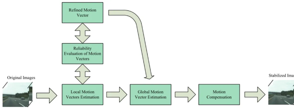
Local Motion Vectors Estimation Reliability Evaluation of Motion Vectors Refined Motion Vector Global Motion Vector Estimation Motion Compensation

Original Images Stabilized Images

Fig. 1.2. Schematic overview of the digital image stabilization developing techniques Fig. 1.2 describes a schematic overview of the digital image stabilization developing techniques. It illustrates the three main issues of DIS developments. These issues are local motion estimation, global motion estimation and motion compensation. The issues presented in this dissertation ,such as motion estimation, which include local motion vectors and global motion vector, and motion compensation will be addressed in separate chapters, each with its own introduction, literature overview and algorithm development. This will make it possible to read each chapter without having to cross-reference to the other chapters.

In chapter 2, we start with the issues of local motion vector estimation and global motion vector estimation. Due to these two issues being mutually related in their information process and development technique, it is hard to separate them. Based on the difference in dynamic and real video characteristics, we propose several techniques to tackle irregular images that contain large moving objects, low-contrast area and lack of features to improve robustness and accuracy. The advantages of our proposed methods in the different functions are:

„ Use representative point matching to dramatically reduce the computation complexity. This makes it possible to build in the regular processors for realization. „ Propose an inverse triangle method to discriminate the reliability of motion

estimation. Based on the inverse triangle method, the related development techniques are:

„ Discriminate the reliability of each local motion vector with respect to each axis.

„ Determine the background-based evaluation area by coarsely detecting the skyline.

„ Determine the optimum representative points for stationary video surveillance system. This will improve the computation efficiency.

„ Use background based evaluation to determine the global motion vector.

In chapter 3, we address the issue of motion compensation. The objective of motion compensation is to reduce the jiggled image phenomenon by generating a compensating motion vector to stabilize the image sequence. The major work in this part is to improve the existing compensation method within the specified requirements such as limited window shifting allowance, panning condition etc. Therefore, an inner feedback-loop integrator and fuzzy inference have been applied to approach the problem. Quantitative evaluation terms, such as motion trajectory and smoothness index, have been developed for final results comparison as well.

In chapter 4, the experimental results of the algorithms developed in chapter 2 & 3 will be interpreted. First, the accuracy of global motion vector estimation will be compared by the root mean square error (RMSE) method. In this part of the experiments, video sequences captured by different applications of hand-held camcorders and in-car video capture devices will be compared with the RPM_FUZZY method. Secondly, motion compensation with the inner feedback-loop integrator will be demonstrated to show the improvements of the motion trajectory and the smoothness index in panning conditions. Furthermore, we describe the results of applying the fuzzy inference algorithm to stabilize the image sequences in various conditions, which can reduce the drawbacks and keep the merits of each motion compensation method.

2. Motion Estimation

2.1. Introduction

Motion estimation is the process of finding optimal or near-optimal motion vectors. Most of these techniques are developed for video compression to increase compression ratios by making better use of redundant information between successive frames. But the motion estimation techniques used in DIS have some differences. The purpose of the motion estimation in DIS is to estimate the reliable global motion vector through three processing steps on the acquired image sequence: (1) evaluation of local motion vectors (LMVs); (2) detection of unreliable motion vector components; (3) determination of the global motion vector (GMV).

The local motion vectors estimation techniques presently used can be divided into three main categories [22], [24], [25]:

„ The intensity gradient techniques [15], [24], [26], [35], [36]. „ The frequency-domain techniques [31], [32], [33], [38]. „ The block matching techniques [5], [10], [27], [29], [30].

The initial hypothesis in calculating image motion with the intensity gradient techniques is that the intensity structures of the local regions are approximately constant for a short duration. In other words, the image luminance is invariant along motion trajectories. If I t x ( , ) is the intensity function of image with respect to t and x .

( , ) ( , ),

I t x ≈I t+δt x+δx (2.1)

where δx is the displacement of the local image region at ( , )t x after time δ . The t

Taylor series expansion of the right hand in (2.1) yields

2 ( , ) ( , ) ( , ) ( , ) I t I t t I t I t t O t δ δ δ δ ∂ + + = + ∇ ⋅ + + ∂ x x x x x x (2.2)

order terms, which are assumed negligible. According to (2.1), ignoring _{O and dividing by} 2 t δ yields ( , ) ( , ) I t 0, I t t ∂ ∇ ⋅ + = ∂ x x v (2.3)

where ( , )∇I t x is the spatial intensity gradient and v is the image velocity. Equation (2.3) is known as the optical flow constraint equation or spatio-temporal constraint equation. As the image intensity changes at a point due to motion, the constraint equation is not sufficient to compute both components of v. That is to say, only the projection of v on ∇I can be determined from (2.3). This problem is known as the aperture problem. Only at image locations where there is sufficient intensity structure, such as the Gaussian curvature, can the motion be fully estimated with the use of the optical flow constraint equation. Therefore, an additional constraint must be introduced to regularize the ill-posed problem and to solve the optical flow. To estimate the exact image motion with optical flow, several conditions have to be satisfied. These are:[24]

„ Uniform illumination

„ Lambertian surface reflectance

„ Pure translation parallel to the image plane

The drawback is that these conditions are not entirely satisfied in scenery images. It can only be assumed that these conditions are held partially in the scene. The degree to which these conditions are partly satisfied determines the accuracy with which optical flow approximates image motion. These techniques also suffer from two serious drawbacks [25]: (1) the smoothness constraint leads to an increased prediction error, especially on moving objects boundaries. (2) the dense motion field (i.e., a motion vector per pixel) requires much overhead information.

A second category of motion vector estimation techniques are based on the use of velocity-tuned filters. It is found that motion-sensitive mechanisms operating on Fourier transform techniques can estimate the motion vector of an image for which other matching approaches would fail. The Fourier transform of a translational intensity of a specified image in (2.1) is

0

( , )_ω ( ) (_δ T _ω),

where Ι k is the Fourier transform of (0, )₀( ) I x and x denotes spatial position. δ is a

Dirac delta function and ,k ω denote spatiotemporal frequency. This yields the optical flow constraint equation in frequency space

0

T _{+ =ω}

v k (2.5)

which means v is a function of k and ω and forms a plane through the origin of the Fourier space. It was shown that velocity-tuned filters could be tuned to ranges of component image velocity. In general, noise robustness is enhanced because the filters can be designed to attenuate noise through time as well as space [39]. If the images are corrupted by frequency-dependent noise, then the Fourier methods are preferred rather than other methods. The phase correlation method is based on the Fourier Shift Theorem and it was originally proposed for the registration of translated images. The method shows strong robustness against the correlated and frequency dependent noise and non-uniform, time varying illumination disturbances [28]. The drawbacks of frequency domain techniques are: (1) They do not provide a means of assigning confidence to the computed velocities [31]; (2)There’s a requirement for a large number of filters to cover frequency space [37]; (3) Numerical differentiation is sometimes impractical because of small temporal support [23].

The block matching techniques are based on the matching of blocks between two images and aim to minimize a disparity measure [25]. These techniques are sometimes called correlation-based techniques or template matching techniques. The basic idea of block matching is defined as a block ( ,B x y_{p p}) around the point p , in which we try to find the best similar block (B x_p+i y, _p+ j) shifted by the integer values in pixels in a search space S

composed by the ,i j such as − < <+ i + and− < <+ j + . The best similar block is defined as a minimum measurement of a distance or a maximum measurement of the correlation between the intensity of an image in the two corresponding blocks. The block matching techniques are the most intuitive and also the most widely applied techniques to compute the motion vector from an image sequence. Different kinds of algorithms use different criteria for the comparison of blocks. Originally, the algorithm to be used for block matching is referred to as the Full Search or Exhaustive Search. In this, each block within a pre-selected search window is evaluated to the current block by disparity measure criteria. The lowest disparity measure value is the best match for the current block. It shows the excellence of quality and simplicity, but it has a really high computation complexity. Therefore, there are several approaches for reducing the computation complexity, such as the three-step search [41], the .new three-step search [42], [43], the four-step search [48], the one-dimensional full search [47] and the

diamond search [44] have been developed to reduce the search positions. Another method is to simplify the matching operations, such as pixel decimation [49], mini-max criterion [51], boundary match [52], pixel truncation [53], representative point matching [5], [6], edge pattern matching [7], [8] and bit-plane matching [9]. In general, these fast algorithms suffer from considerable peak signal-to-noise ratio (PSNR) degradation compared to full-search block matching algorithm (FSBMA), especially when the motion field is large and complex [30]. One of the motion estimation problems is the reliability measure. The confidence measures can indicate the reliability of estimated motion vectors which may suffer from transparency, occlusion, lacking features, repeated patterns or low contrast. The confidence measures can be used to screen the unreliable motion vectors during the estimation process. In the digital image stabilization applications, some of the motion estimation properties should be emphasized such as (1) low computation complexity; (2) large motion estimation areas that are larger than the macroblocks with a size of 8x8 or 16x16, which are used in MPEG video compression; (3) full usefulness of motion estimation information; (4) high reliability of motion vectors; (5) background based motion vectors.

In this chapter we present the details of motion estimation for digital image stabilization. Firstly, we proposed the architecture of the DIS system, the block diagram of motion estimation and then addressed the evaluation of local motion vectors by the representative point matching method. Secondly, we discussed the detection of irregular conditions in the image sequence. In this section, the inverse triangular method is introduced to measure the reliability of local motion vectors. Based on this method, the selection of the representative point amount is discussed. Thirdly, the next section addressed the generation of refined motion vector (RMV) to tackle the ill-conditions of image sequences.

2.2. Motion Estimation

2.2.1. Motion Estimation Architecture

The architecture of the proposed DIS system, shown in Fig.2.1, includes two processing units, the motion estimation unit and the motion compensation unit. The motion estimation unit consists of three estimators: the local motion vectors (LMV), the refined motion vector (RMV), and the global motion vector (GMV) estimators. The motion compensation unit consists of the compensating motion vector (CMV) estimation and image compensation. In the first part of motion estimation, as shown in Fig. 2.2, the LMVs and RMV estimation is to generate the LMVs and RMV for global motion vector estimation. The LMVs can be obtained from the correlation between two consecutive images by the representative point matching (RPM) algorithm. The RMV can be obtained from LMVs by evaluating the corresponding confidence indices through the irregular condition detection and the proposed RMV generation algorithm.

LMVs and RMV Estimation

RMV

LMVs GMV Compensating Motion Vector Estimation

Image Compensation CMV

Original Images Compensated Images

Motion Estimation Motion Compensation

Global Motion Vector Estimation

Fig. 2.1. System architecture of the proposed digital image stabilization technique

Representative Point Matching (RPM) Representative Points Buffer LMVs Estimation ( Four regions) Minimum Projections of x and y Directions ( Four regions) Inverted Triangle Method Irregular Condition Detection Generation of RMV RMV LMVs

2.2.2. RPM and Local Motion Estimation

It has been demonstrated that a local approach that uses a regional matching process is more robust and stable than a direct global matching process [50]. This means that using the local motion vectors estimated by the divided regions to determine the global motion vector is more robust and stable than a direct approach. There is also a tradeoff for the size of the divided region. Reducing the size of the divided region increases the robustness, but the size of the divided region should be sufficiently large enough to hold the average distribution. If we want to divide the image so that the horizontal and vertical components have the same partitions, it should be divided into_{n regions. More divided regions will increase the} 2

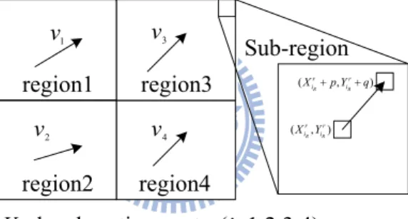
computational cost to estimate the local motion vector for each region. Therefore, we only divided the image into four regions, as shown in Fig. 2.3, for the RPM method and it can cover various situations in the DIS applications by combining the proposed inverse triangle method and the adaptive background evaluation model.

1 v v3 4 v 2 v ( , ) R R r r i i X Y ( , ) R R r r i i X +p Y +q region1

Vi : local motion vector(i=1,2,3,4)

region3

region2 region4

Sub-region

Fig. 2.3. Division of image for local motion vector estimation

Each region is further divided into 30 sub-regions (with each side of 5 rows×6 columns) and the central pixel of each sub-region is selected as the representative point to represent the pattern of this sub-region. This layout is based on the size of images captured by the regular imaging devices, such as 640×480 or 320×240. In order to make the representative points equally distributed in spatial, the ratio of row and column should be maintained by as close to 3:4 as possible.

Then the correlation calculation of RPM with respect to representative point (X Y is _r, )_r performed as 1 ( , ) N ( 1, , ) ( , , ) i r r r p r q r R p q I t X Y I t X ₊ Y₊ = =

∑

− − , (2.6)

of the representative point (X Y_r, )_r at frame( 1)t− , and R_i( qp, ) is the correlation measure for a shift ( qp, ) between the representative points in region i at frame( 1)t− and the relative shifting points at frame( )t . Assuming R_iMin is the minimum correlation value in region i, i.e.

, ( ( , ))

=

iMin _{p q} i

R Min R p q , the shift vector v that produces the minimum _i

correlation value for region i represents the local motion vector of this region, i.e., ( , ), for ( , )

i i iMin

v = p q R p q =R . (2.7)

2.2.3. Irregular Condition Detection

By analyzing the curves of correlation values corresponding to image sequences with various conditions, it is found that the curve of correlation values is related to the reliability of motion detection. Figs. 2.4 and 2.5 show the various correlation curves corresponding to different video images with different conditions. Fig. 2.4 is a video image captured by a hand-held camcorder of a daily life scene. Fig. 2.5 is a video image captured by an in-car video camera of an outside scene. It is found that the irregular conditions detected in daily life scenes can be detected in in-car applications as well. Fig. 2.4 (a) and 2.5 (a) show a normal condition where the peak of correlation is obvious in each region. In Fig. 2.4 (b) and 2.5 (b), the curves look like a valley. This means only one dimension of correlation data is reliable and it lacks of feature in the other direction. Fig 2.4 (b) is short of features in the x direction. On the contrary, Fig 2.5 (b) is short of features in the y direction. Fig. 2.4 (c) and Fig. 2.5 (c) show examples with repeated patterns. Fig. 2.4 (c) is an image of an office partition filled with grid-hole patterns, especially on region 2 and 4, which causes multiple peaks on these regions. Fig. 2.5 (c) is an image of a brick wall with a fence in the bottom area, and it also causes multiple peaks in the correlation curves, especially within region 1 due to the pure bricks that are repeated in this area. Fig. 2.4 (d) represents the condition of a moving object; a bear moves from the left side to the right side of the image sequence. It causes double peaks in the curve of region 2 and the value of RiMin is larger than the value of a normal image, such as Fig. 2.4 (a). Fig. 2.5 (d) represents an image sequence of a motorcycle moving from the right side to the left. It causes double peaks within region 1 of the curve and the value of

iMin

contains a white wall on the right side of the image. Obviously, it is very hard to distinguish the peak from the correlation curve in region 4. Fig. 2.5 (e) contains a large low-contrast area (blue sky) on the upper left corner of the image. It is also hard to distinguish the peak in region 1.

Although the curve of correlation values is related to the reliability of motion detection, it is still too complex to directly use these curves to evaluate the reliability of motion detection. Therefore, we propose a strategy that combines the minimum projections of correlation curve in x and y directions (minimum projections) and the inverse triangle method to detect the irregular conditions from each region. The mathematical expression of minimum projections can be written as:

_ min( ) min ( , ) _ min( ) min ( , ) i _q i i _p i x p R p q y q R p q = = , (2.8)

where _ min( )x_i p and y_i_ min( )p are the minimum projections of correlation curve

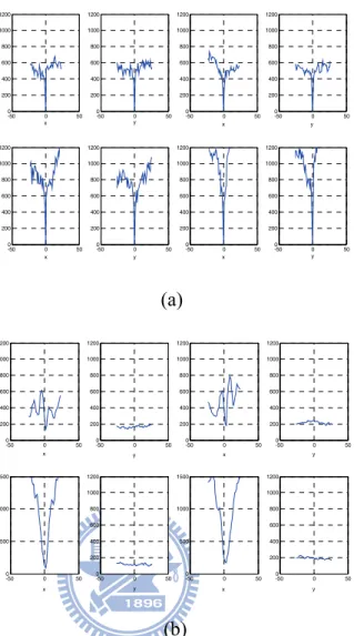
in x and y directions in region i , respectively. Fig. 2.6 shows the examples of minimum

projections of the correlation curve in x and y directions. Fig. 2.6(a) is the minimum projection of Fig. 2.5(a), that is regular and the determination of motion vector in each region is clear and consistent. Fig. 2.6(b) is the minimum projection of Fig. 2.5(b), which shows a lack of features in y direction (horizontal). The values of the minimum projection of correlation curve in y direction are within a small range and erratic with multiple peaks so that the determination of the minimum value is very hard.

In order to determine the reliability of motion vector easily, the feature extraction of reliability is performed by the proposed inverse triangle method through the minimum projections in x and y directions to obtain the reliability indices. Fig. 2.7 shows the illustration of the inverse triangle method. In the first step, we find T_i_ min that represents the global minimum of the minimum projection curve in region i and can be calculated by Eq. (2.9).

In the second step, we calculate S and _xi S by Eq. (2.10), where _yi offset is the

altitude of the inverse triangle. n and _xi n are defined as the numbers of _yi S and _xi S , _yi

respectively (see Eq. (2.11)). d and _xi d are defined as the distances of two vertexes of the _yi

base of the inverse triangle obtained by Eq. (2.12). The cost level of x and y directions are

calculated by Eq. (2.13). The higher cost level means a lower confidence level. Since the condition of multiple peaks seriously degrades and affects the determination of reliability, the

reliability. The example shown in Fig. 2.7 is a curve with twin peaks which will get the penalty of d_xi −n_xi. In the third step, we determine the confidence indices of x and _i y in _i

region i through a threshold denoted as TH . The lower cost level represents a higher reliability. In the final step, summing up the counts of reliable motion components of x and y

in the four regions as Eq. (10), we get Num x and ( )_i Num y( ), 1 ~ 4 _i i= .

Step 1. Find global minimum T_i _ min from _ min( ) or _ min( )x_i p y_i q

_ min min( _ min( )) or min( _ min ( ))

i i i

p q

T = x p y q (2.9)

Step 2. Calculate the cost level, _ costx_i andy_i_ cost { | _ min( ) _ min } { | _ min( ) _ min } xi i i yi i i S p x p T offset S q y q T offset = < + ⎧⎪ ⎨ _{= < +} ⎪⎩ (2.10) number of number of xi xi yi yi n S n S = ⎧⎪ ⎨ ₌ ⎪⎩ (2.11) max min max min xi _P xi _P xi yi _q yi _q yi d S S d S S = − ⎧⎪ ⎨ _{= −} ⎪⎩ (2.12) _ cost 2 _ cost 2 i xi xi i yi yi x d n y d n = − ⎧⎪ ⎨ _{= −} ⎪⎩ (2.13)

Step 3. Set the threshold,TH , for determining the reliability indices

If _ cost x_i < TH Then (2.14) i x is reliable Else x is unreliable _i End if . y_i_ cost < TH Then y is reliable _i Else y is unreliable _i

End if

Step 4. Calculate the numbers ofx and_i y in four regions _i

( ) sum of ( is reliable) ( ) sum of (y is reliable) i i i i Num x x Num y = ⎧ ⎨ ₌ ⎩ (2.15) 1 ~ 4 i=

(a)

(b)

(c)

(d)

(e)

Fig.2.4. Various correlation curves that correspond to image sequences with different conditions.(I) (a) A normal condition (b) Features lacking in the vertical direction (book) (c) Repeated patterns (office) (d) Moving object (bear) (e) Large low-contrast area (white wall) Video images captured by a camcorder in daily life scene.

(a)

(b)

(c)

(d)

(e)

Fig.2.5. Various correlation curves that correspond to image sequences with different conditions (III). (a) A normal condition (b) Features lacking in the horizontal direction (gate) (c) Repeated patterns (brick) (e) Moving object (motorcycle) (f) Large low-contrast area (sky) Video images captured by an in-car video camera during outside scene.

-50 0 50 0 200 400 600 800 1000 1200 x -50 0 50 0 200 400 600 800 1000 1200 y -50 0 50 0 200 400 600 800 1000 1200 x -50 0 50 0 200 400 600 800 1000 1200 y -50 0 50 0 200 400 600 800 1000 1200 x -50 0 50 0 200 400 600 800 1000 1200 y -50 0 50 0 200 400 600 800 1000 1200 x -50 0 50 0 200 400 600 800 1000 1200 y (a) -50 0 50 0 200 400 600 800 1000 1200 x -50 0 50 0 200 400 600 800 1000 1200 y -50 0 50 0 200 400 600 800 1000 1200 x -50 0 50 0 200 400 600 800 1000 1200 y -50 0 50 0 500 1000 1500 x -50 0 50 0 200 400 600 800 1000 1200 y -50 0 50 0 500 1000 1500 x -50 0 50 0 200 400 600 800 1000 1200 y (b)

Fig. 2.6. Examples of minimum projections of correlation curve from x and y directions in four regions. (a) Regular image sequence. (b) Ill-conditioned image sequence.

xi d xi n offset _ min i T

2.2.4. Determination of Representative Point Amount

Determining the representative point amount is quite an issue when using the RPM method. How many points are necessary to determine the local motion vector? Trial and error is one approach to get a better number, but it is neither efficient nor scientific. The reliability measure by inverse triangle method can be used for this issue. The cost value evaluated by Eq. (2.13) is an index of reliability. The higher cost level indicates a lower reliability. According to our experimental results, a threshold of cost value set at 18 can get the reliable motion vectors from our experimental video sequences. Fig. 2.8 shows the experimental result of calculating the cost level by using a different number of representative points. This is the averaged testing result for the experimental video sequences used in chapter 4. It can be found that if the number of the representative points is larger than 30, the cost level will get down to the threshold and almost all the motion vectors calculated by the RPM method are reliable. In other words, in this case, the cost level will be good enough at the lower value in regards to higher reliability. In order to keep low computation time complexity, 30 representative points are used in our system.

0 10 20 30 40 50 60 70 80 90 0 5 10 15 Threshold20 25 30 35 40 45 50

Amount of representive point

C o st le ve l

Fig. 2.8. The experimental result of calculating the cost level (that is an index of reliability defined in Eq. (2.13)) by using a different number of representative points.

2.2.5. Optimization of Representative Points

In the fixed-type video surveillance system, the DIS process can be divided into two sub processes: the initialization process and the compensation process. The main characteristics are: (1) the background is stationary; (2) the fluctuation of an image is caused by wind

people walking can cause partial local motion in the image, which will disturb the global motion detection. The initialization process can optimally select the representative points from the background image by the difference measurement. It can increase the reliability of motion vector detection.

The optimization process consists of difference measurement and optimization of representative points. First, the difference measurement derives a difference matrix for each selected representative point. Second, the optimization process chooses the optimal representative point among those points in the corresponding sub-region.

The difference measurement is based on the concept of the aforementioned RPM method. Each representative point is selected from a point of the corresponding sub-region, which can be expressed as( r, r)

l l

X Y , where lis the index of representative points in each sub-region, r is the index of the sub-region. The difference matrix of each representative point can be written as

( , ) ( , ) ( , ) , 1_{total rows} 1_{total rows of sub-region,} 2 2

1_{total columns} 1_{total columns of sub-region.} 2 2 r r r r r l l l l l DIF p q I X Y I X p Y q p q = − + + − ≤ ≤ − ≤ ≤ (2.16) where ( , r, r) l l

I t X Y is the intensity of the representative point( r_R, _Rr)

l l

X Y , and r( , )

l

DIF p q is the difference matrix corresponding to representative point( r_R, _Rr)

l l X Y .

The difference matrix expresses the degree of similarity between the representative point and the neighborhood. The mean value of difference matrix can globally represent the similarity between the representative point and the neighborhood, which is

( ( , ))

r r

l l

M =mean DIF p q , (2.17)

where lis the index of the representative point in each sub-region, r is the index of the sub-region. The largest r

l

M means the representative point is less similar to its neighborhood, i.e. the best candidate for the representative point, which can be expressed as

( ) r r R _l l i =Max M , (2.18) where r R

l is the index of the optimal representative point in the sub-region r. If the values of r

l

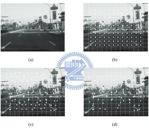
M in sub-region rare smaller than a pre-defined threshold, the representative point will be neglected due to the lesser difference between itself and the neighborhood. Fig. 2.9(a) shows the background of the video surveillance image captured from the road scene. Fig. 2.9(b) shows the locations of traditional representative points, which are usually located within the

centers of the corresponding sub-regions respectively. The horizontal and vertical lines are formed to separate the sub-regions for illustration. Fig. 2.9(c) shows the locations of the optimal representative points. Each point is selected by the most significant point (highest r

l M ) in the sub-region. The optimal representative points can increase the confidence index through the cost level calculation by Eq. (2.13). After neglecting the insignificant points by that r

l M are smaller than pre-defined threshold, the remaining representative points are shown in Fig. 2.9(d). The neglecting insignificant points can reduce the computation complexity without affecting the confidence index of motion estimation.

(a) (b)

(c) (d)

Fig. 2.9. The illustration of optimal representative point selection method. (a) The original image. (b) The traditional representative points. (c) The optimal representative points. (d) The optimal representative points after neglecting insignificant points.

2.2.6. Generation of Refined Motion Vector

Irregular motion vectors can be detected and excluded by using the minimum projection and inverse triangle method; however, image sequences with ill conditions, such as a lack of features, a large low-contrast area, a moving object or a repeated pattern, may contain fewer available MVs (most of the MVs are irregular) in the four regions. Therefore, a recombination of these available components of regular MVs is necessary to form a refined motion vector

(RMV). To solve this problem, a median function is used to extract a motion vector with respect to each direction for the ill condition. The calculation to determine the RMV is described as follows in detail.

Case 1. If Num x t( ( )) 4_i = then

_ ( ) ( _ ( ), _ ( ), _ ( ), _ ( ), ( 1))

refined x a x b x c x d x x

V t =Med V t V t V t V t GMV t− Case 2. IfNum x t( ( )) 3_i = then

_ ( ) ( _ ( ), _ ( ), _ ( ))

refined x a x b x c x

V t =Med V t V t V t Case 3. IfNum x t( ( )) 2_i = then

_ ( ) ( _ ( ), _ ( ), ( 1))

refined x a x b x x

V t =Med V t V t GMV t− (2.19) Case 4. If Num x t( ( )) 1_i = then

_ ( ) _ ( )

refined x a x

V t =V t Case 5. If Num x t( ( )) 0_i = then

_ ( ) ( 1)

refined x avgx

V t = ×γ GMV t−

whereNum x t is the number of x components of reliable LMVs, ( ( ))_i V_{refined x_} ( )t is the x

component of RMV, V_{a x_} ( )t , V_{b x_} ( )t , V_{c x_} ( )t , and V_{d x_} ( )t represent x components of

reliable LMVs in the different regions, respectively, Med( ) is the function of median operation, ( 1)GMV t_x − is the x component of the previous GMV, t is frame number, γ is attenuation coefficient, 0< < . The γ 1 GMV_avgx( )t can be calculated by

( ) ( 1) (1 ) ( )

avgx avgx x

GMV t =ζGMV t− + −ζ GMV t , 0< <1ζ . (2.20)

Then we apply the similar process to obtainV_{refined y_} ( )t . The resultant RMV is represented by

_ _ ( ) ( ) ( ) refined x refined refined y V t V t V t ⎡ ⎤ = ⎢ ⎥ ⎣ ⎦. (2.21)

2.2.7. Global Motion Estimation

The objective of global motion vector estimation is to determine a motion vector from the existing data that has been evaluated from the motion estimation process. In a practical video sequence, it always suffers from moving objects, repeated patterns etc. The LMV in

each region may represent the global motion vector, the moving object motion vector, or even the error vector, respectively. The error vector may be caused by an ill condition, a repeated pattern, or the mixture of global and moving object motion. A reliable global motion vector is essentially selected from the LMVs and RMV. However, in the worst case, i.e. if the LMVs and RMV are all faulty, this will induce a worse result after compensation compared with the original images. Therefore, if the evaluation includes the zero motion vector (ZMV), it can prevent the occurrence of this case. Similarly, for an image sequence with constant motion in the scene, it will induce a worse result if it is compensated by ZMV or error motion vector rather than by the average motion vector (AMV). In the proposed DIS technique, the seven motion vectors, which include the four LMVs, the RMV, the ZMV, and the AMV, which are referred to as pre-selected motion vectors (pre MV ), are employed to estimate the GMV of _ the current frame. In general, one of LMVs is the highly probable GMV for the regular image. The RMV is the highly probable GMV for the ill-conditioned image. The ZMV can prevent a worse compensation result caused by the unreliable MVs, and the AMV is useful for the constant motion of the car. In addition, if the image sequence contains a large moving object, the determination of global motion is troublesome because the determined motion vector probably switches between the background and the large moving object or it is totally dominated by the large moving object. In this case, it will lead to artificial shaking and cause an important challenge in DIS.

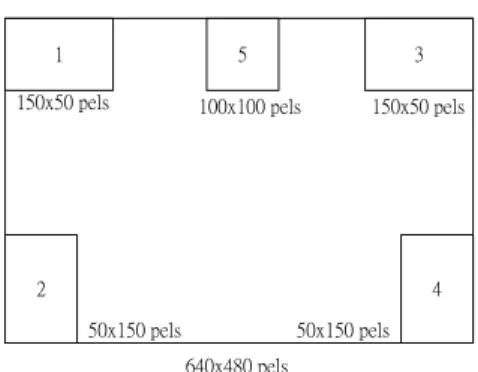
2.2.7.1. Background Based Peer to Peer Evaluation

In this dissertation, a background-based evaluation function is proposed to overcome the large moving object problem. Fig. 2.10 shows the areas for the background-based evaluation. Five regions are selected to evaluate the result, which are located on the surrounding areas of the image. The reason is that, in most cases, the foreground object is located in the center of the image, so the surrounding areas of the image are the best candidates for background detection. The estimation of the GMV is calculated by the summation of absolute difference (SAD), , , ( 1, , ) ( , , ) , 1 5, 1 7, i i B c c c X Y B SAD I t X Y I t X X Y Y i c ∈ = − − + + ≤ ≤ ≤ ≤

∑

(2.22)

where I t( −1, , )X Y is the intensity of the point ( , )X Y at frame t-1, Bi is the i-th background region in the image, X Y_c, _care the components of the seven pre-select motion vectors (pre MV_ _c) in x and y directions.

Eachpre MV_ c can obtain it’s SADB ci, in each region. The smaller SADB ci, represents the

higher probability of the desired motion vector among theses pre-selected motion vectors. The score for eachpre MV_ _c in region i is denoted asSi c, , which is the order of the SADB ci, value, and the higher SAD_{B ci,} indicates the higher score. The total score for each pre MV_ _c can be

obtained by 5 , 1 c i c i S S = =

∑

. (2.23)

Five-region peer-to-peer evaluation can prevent the situation that some partial high-contrast image regions dominate the evaluation result. In this algorithm, each region has an equal priority to determine the result. In (14), S_c is the index to determine the GMV. The

_ c

pre MV with the smallest Sc is the desired GMV and it can be expressed as

GMV=pre MV_ _i, for arg(min _c)

c

i= S . (2.24)

According to these sophisticated evaluation areas, the evaluation function can detect the attributed background motion vector precisely in most circumstances.

2 4

1 5 3

50x150 pels 50x150 pels

150x50 pels 100x100 pels 150x50 pels

640x480 pels

Fig. 2.10. Areas for background detection and evaluation.

2.2.7.2. Skyline Detection

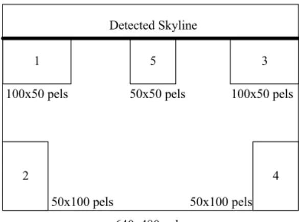
To improve the robustness of the global motion vector estimation, the adaptive background-based evaluation function is proposed. Firstly, the skyline detection will be

performed. Then, five regions, based on the estimated skyline, are selected to evaluate the result. In most outdoor applications, such as in-car video capture, the pixels of the area above the skyline are low contrast. The skyline detection can prevent an invalid result due to some of the five regions located on the low-contrast area. Selecting the regions surrounding the boundary of the image to evaluate the obtained motion vector can avoid the disturbance of moving-object effects for global motion vector estimation. Fig. 2.11 shows the adopted areas for the adaptive background-based evaluation according to detecting the skyline. The proposed skyline detection algorithm combines RPM correlation evaluation, minimum projection, and the inverse triangle method. First, we calculate the absolute differences between the representative point at frame( 1)t− and the corresponding neighborhood pixels in the same sub-region at frame( )t by Eq. (2.25) that is regarded as the intermedium of Eq.

(2.6),

, ( , ) ( 1, , ) ( , , )

i j i j i p j q

C p q = I t− X Y −I t X₊ Y₊ , (2.25) where( , )i j denotes the position of one sub-region with respect to the row and column as

shown in Fig. 2.12. There are 120 sub-regions (10 rows x 12 columns in this paper). ( , )X Yi j is the coordinate of the representative point in the ( , )i j sub-region, ( 1,I t− X Y_i, )_j is the intensity of the representative point ( , )X Y at frame( 1)_{i j} t− , and ( , )p q is a shifting vector

within the sub-region. Then we can derive the correlation curve for detecting the skyline by calculating , 1 1 ( , ) l M ( , ) l i j i j C p q C p q = = =

∑ ∑

, (2.26)

where M is the total number of sub-regions in the horizontal axis (M =12), l represents the l-th row of the sub-regions. Initially, l=1 and the minimum projection and inverse triangle method presented in Eq. (2.9) ~ (2.13) are applied to C p q to get the confidence l( , ) index in the horizontal direction. The cost level is relatively high when the corresponding area is a low-contrast area such as the sky. If the level is lower than the presetting threshold then we stop the evaluation process and the horizontal position of the representative points of the sub-regions located in the last row of C p q is defined as the coarse skyline. Otherwise, _l( , ) we set l l= +1and continue the evaluation of ( , )C p q till the level is lower than the l

presetting threshold. Fig. 2.13 shows the results of skyline detection in the video sequence taken from the highway. The coarse skyline is used to adaptively layout the background-based

evaluation blocks located on the higher contrast area. It improves the robustness of global motion vector estimation in image stabilization applications.

2 4

1 5 3

50x100 pels 50x100 pels 100x50 pels 50x50 pels 100x50 pels

640x480 pels Detected Skyline

Fig. 2.11. Areas for the background-based evaluation adapted by the detected skyline.

Fig. 2.12. Skyline detection algorithm is to combine RPM correlation evaluation, minimum projection and inverse triangle method.

(a) (b) Fig. 2.13. Skyline detection applies on the in-car video sequence taken from the highway.

2.3. Summary

In this chapter we address the related research works of motion estimation and the advantages/disadvantages of various algorithms in more detail. To detect irregular conditions, we proposed an inverse triangle method to measure the reliability of evaluated motion vectors according to the correlation curve. The inverse triangle method evaluates the cost value in x and y directions for each motion vector, respectively, and then uses the cost value of each component of the motion vector to generate the refined motion vector. It can positively contribute to determinate the global motion vector in ill-conditioned images that have a lack of features, repeated pattern etc.

The determination of the representative point amount is also addressed by using the inverse triangle method. Based on this result, the representative point amount is set on 30 for each estimation region. In the fixed-type video surveillance system, the optimization of selecting the representative points from the background image by the difference measurement can increase the reliability of motion vector detection. The optimization process consists of the difference measurement and the optimization of the representative points. First, the difference measurement derives a difference matrix for each selected representative point. Second, the optimization process chooses the optimal representative point among those points in the corresponding sub-region.

Skyline detection and background based peer to peer evaluation have been proposed to improve the robustness of the global motion estimation. The background based peer to peer evaluation solves the large moving object problem and reduces artificial shaking in DIS. The skyline detection uses the coarse skyline to adjust the background-based evaluation area. It can prevent an invalid result due to some of the five regions located in the low-contrast area.

The DIS system combines with the aforementioned motion estimation approaches and can adapt to various conditions such as daily, in-car and surveillance applications.

3. Motion Compensation

3.1. Introduction

Motion compensation used in video compression is a technique that describes a picture in terms of translated copies of portions of a reference picture, often 8x8 or 16x16-pixel blocks. The objective is to increase compression ratios by making better use of redundant information between successive frames [54]. But motion compensation used in DIS is a technique for generating the compensating motion vector. This will compensate and shift the current picking window, accordingly, to obtain a smoother image sequence. Most of the research in the field of digital images stabilization is concentrated in the motion estimation part of the system. But motion compensation still plays a decisive role in the DIS system, especially in practical applications. Accumulated motion vector estimation and frame position smoothing (FPS) are the two most popular approaches to generate the compensating motion vector. J. K. Paik proposed the accumulated motion vector method in 1992. The computation procedure is given by [7]:

( ) ( ( 1)) ( ( ) (1 ) ( 1))

CMV t =k CMV t− + αGMV t + −α GMV t− (3.1) where t represents the frame number, 0< <k 1 and 0≤ ≤α 1. The constant k is used for

smooth panning. The constant α is used to filter out the unexpected noise effect. The increase in k causes the decrease in unwanted shaking effect but the increase in the value of CMV leads more allowance to compensate. It means that, in the definite allowance, it may not fully stabilize the image sequence by the CMV, especially in a high panning condition.

The accumulated motion vector estimation needs to compromise stabilization and intentional panning (constant motion) preservation since the panning condition causes a steady-state lag in the motion trajectory [20]. The FPS accomplished the smooth reconstruction of an actual long-term camera motion by filtering out jitter components based on the concept of designing the filter with appropriated cut-off frequency. The disadvantage of FPS is that it does not guarantee the availability of the determined compensating motion vector when the specified-bound is restricted for preserving the effective image area in the DIS applications.

3.2. Compensating Motion Estimation

3.2.1. Motion Trajectory

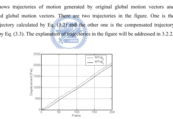
To easily illustrate CMV estimation afterwards, the motion trajectories will be introduced first. These can then be calculated to analyze the problem that will be addressed in 3.2.2. The motion trajectories can be obtained by

1 ( ) t ( ) o i MTraj t GMV i = =

∑

, (3.2) 1 ( ) t ( ) ( ) c i MTraj t GMV i CMV t = ⎛ ⎞ =_{⎜ ⎟}− ⎝

∑

⎠ , (3.3)

where ( )MTraj t and _o MTraj t are the original and the compensated motion _c( ) trajectories of the image sequence at frame( )t .

Fig. 3.1 shows trajectories of motion generated by original global motion vectors and compensated global motion vectors. There are two trajectories in the figure. One is the original trajectory calculated by Eq. (3.2) and the other one is the compensated trajectory calculated by Eq. (3.3). The explanation of trajectories in the figure will be addressed in 3.2.2.

Fig. 3.1. Trajectories of motion generated by original global motion vectors and compensated global motion vectors. The compensated motion trajectory generation method in (3.1)

3.2.2. Quantitative Evaluation

The shaking effect of images can be evaluated by the summation of absolute differences of momentums within every two consecutive frames. The mass of an image can be set as a constant, such as one, for simplicity, or a value from zero to one, according to the degree of shaking in the images measured by human visual perception. The smoothness index (SI) is proposed to quantitatively evaluate the performance of different DIS algorithms and it is defined as

∑

∑

= = − − × − = Δ − = N t N t t GMV t GMV m N t m N SI 2 2 ) 1 ( ) ( 1 1 ) ( 1 1 , (3.4) where t is the frame number, N is the number of total frames, m is the mass of the

image, and Δm(t) is the change rate of the absolute value of momentum. The lower SI means less shaking components in the image sequence and it represents a smoother effect.

3.2.3. Compensation with Inner Feedback-Loop Integrator

The compensating motion vector (CMV) estimation is used to generate CMVs for removing the undesired shaking motion, but still keep the steady motion in the image sequence. The estimation follows the conventional compensating motion vector estimation by (3.1) as CMV t( )=k CMV t( ( 1)) (− + αGMV t( ) (1+ −α)GMV t( 1))− .

The CMVs in Fig. 3.1 are generated by the conventional method shown in Eq. (3.1). Obviously, ( )MTraj t has tremendous lag compared to _c MTraj t due to the constant _o( ) motion effect. Fig. 3.1 and 3.2 show the performance comparison of three different CMV generation methods applied to a video sequence with constant motion and jitter in the image. There are two trajectories in each subfigure; one is the original trajectory calculated by Eq. (3.2) and the other one is the compensated trajectory calculated by Eq. (3.3). The CMVs in Fig. 3.1 are generated by the conventional method shown in Eq. (3.1). Obviously, MTraj t _c( ) has tremendous lag compared to MTraj t due to the constant motion effect. The CMV _o( ) probably exceeds the window shifting allowance such that the available effective image area during the compensation process is reduced. The CMVs in Fig. 3.2(a) are generated by Eq. (3.1) with clipper function as

(

)

1

( ) ( ( )) ( ) ( )

2