A DISTRIBUTED STATE ESTIMATOR FOR ELECTRIC-POWER SYSTEMS

(1)

I 551

Transactions on power Systems, Vol. 7, No. 2, May 19g2

A DISTRIBUTED STATE ESTIMATOR FOR ELECTRIC POWER SYSTEMS

S.-Y. Lin

Department of Control Engineering National

Chiao

lhng University

IIsindiu, TAIWAN, R0.C. Abstract - In this paper, we develop a theoretically robust

and computationally efficient distributed state estimator, which is t o solve the WLS problem by using distributed computation,

for the power system. This distributed state estimator aims a t its utilization in the decentralized control, and it is executing in

a data communication network which is assumed to be topologically the same and physically in parallel with the power network. Along with this state estimator, we can obtain several attractive satellite functions which include (1) reduction of the time-skew

problem, (2) being free from the power network topological er-

ror, (3) easy identification of the unobservable states and (4) bad data detection and identification. We have analyzed the computation complexity of this distributed state estimator. Moreover, we have also simulated this state est,imator on several cases of the IEEE 30-bus system. The numerical accuracy of the siniula- tion results are satisfactory, and t,he estimated computation t,ime including the communication delay demonstrates the excellent computational performance of the distributed state estimator.

INTRODUCTION

There has been a long history in the development of power system state estimators since 1970 when Schweppe and his col-

league first posed the problem [l]. Ty ical state estimators for

centralized control were summarized in

f3]

by Bose and Clements. Evolving with the hierarchical control strategies of power systems, several state estimators for hierarchical control were developed (e.g., p],[5]), and they were discussed in [6] by Van Cut-

sem and Ri bens-Pavella. Nowadays, the decentralized control technologies has made continual progress [8]-[lo]. Although the

decentralized control techniques have not yet applied to power system, however, the trend is unavoidable because the decentralized control has obvious advantages over the centralized and hierarchical control for the large-scale interconnected systems [lo].

This draws enough attraction t o develop the distributed state estimator.

This paper presents a theoretically robust and computationally efficient distributed state estimator under the assumption

of the existence of a high speed data communication network. The proposed distributed state estimator is to solve the weighted least square (WLS) state estimation problem by using distributed computation. We begin by combining the recursive quadratic programming with the dual method (RQPD) to solve the WLS problem [ll]. This RQPD method is robust because of its global convergence property. It is also computationally efficient due to its parallel computation nature. Furthermore, because of its complete decomposition property, it can be executed in a data communication network by distributed computation.

The above mentioned data communication network is assumed to be topologically the same and physically in parallel with the power network. The assumption is justified because (a) the cost

91 SM 4 6 3 - 0 PWRS A paper recommended and approved by the IEEE Power System Engineering Committee of the IEEE Power Engineering Society for presentation at the IEEE/PES 1991 Summer Meeting, S a n Diego, California July 28

-

August 1 , 1991. Manuscript submitted January 22, 1991; made available for printing June 5 , 1991.

of computer and memory continues to decline, and ( b ) the avail- ability of data communication network and the technology of optical fiber transmission keep evolving. These two factors, pointed out in [13] by Gaushell and Darlington, will accelerate the t.rend

toward the distributed processing of power system. Moreover, a trial of integrating t,he communication net,work and the power system is ongoing [14].

Along with the developed distributed state estimator, we can obtain several attractive satellite functions which include the reduction of the time-skew problem, the topological error free power network model, the easy identification of the unobservable states and t.he bad data detection and identification. Details of these functions are described in this paper.

We have analyzed the computation complexity of the developed distributed state estimator. The result shows that because of its inherent property of parallel computa.tion and the nature of sparse-matrix technique, this state estimator achieves tremendous computational time saving. We have also simulated this state estimator on several cases of the IEEE 30-bus system. The simulation results are satisfactory, and the estimated time which includes the computation time and the communication de- lav outdavs the conventional WLS state estimator by the Newton method [2].

The conceDt of distributed Drocessine: had been applied for state estimatiAn by Zaborszky e;. al., in [r5] and Brice and Kavin

in [ 1 6 . However, Our distributed state estimator differs from

scheme is mainly carried out in the control center. Although the estimator based on relaxation method in [16] can be considered as

a distributed state estimator, it is not clear how their distributed computation is arranged.

the U

I

t r a fast state estimator in [15] because their estimation

WLS STATE ESTIMATION PROBLEM

Mathematically, the static-state estimation problem of an n- bus power system is described below as a WLS problem

min q T ~ - ' q

subject to: where

2 = h ( l )

+

q

I: 2n dimensional vector of state variables-voltage mag-

nitude U and phase angle 0,

z : m dimensional vector of measurements,

h: m nonlinear measurement functions,

71: m dimensional random vector of measurement errors,

R: m x m diagonal covariance matrix of measurement errors

71.

T H E RQPD METHOD

In order t o solve (1) by the distributed computation, we need a method with property of decomposition up to bus level. From here on, such decomposition property will be addressed as complete decomposition. For the consideration of complete decomposition, the dual method is a good candidate but it requires that the problem t o be solved should be separable and has a positive definite Hessian matrix [17]. Clearly, (1) is highly nonlinear and nonseparable. But the quadratic approximate subproblem of ( l ) , a t any E-th iteration of the recursive quadratic programming method, is separable as shown in (2) [18].

3.0001992 IEEE 0885-8950/92$0

(2)

552

I "

z,: the measurements made at bus z such as the bus injec- tion power or voltage magnitude at bus 2 , or the line flows from bus i ,

hf: = h,(z'), a subset of h ( z k ) corresponding to z,,

x k : the values of the states z, of bus z at the k-th iteration

or the recursive quadratic programming method,

H i : 8 h f J 8 x l , H:: 8 h f J a z i ,

J,: the set of buses directly connected to bus z in the real- time power network,

q,: subvector of q corresponding to t,, r,: diagonal submatrix of R corresponding to q,, 7 : weighting constant, a positive real number, d x k : = ( d x ~ , d z ~ , . - . , d z ~ ) , the variables of (2). This separable quadratic approximate subproblem (2) has a positive definite Hessian matrix. Hence, it is ideally suited to the dual method to achieve the complete decomposition.

Therefore, a new iterative method which combines the recur- sive quadratic programming with the dual method (RQPD) to solve (1) can be described below:

zk+' = g k

+

p k ( d z k ) * ₍₃₎

where (dz'))' is the optimal solution of (2) which will be solved by the dual method, and the stepsize

pk

is determined by

flk

= arg{min[z

-

h ( z k

+

/ ? ( d ~ ~ ) ' ) ] ~ R - ' [ z - h ( z k

+

p ( d z k ) * ) ] } . 0

In the following, we will illustrate how the dual method solve The dual problem of (2) is described below:

(2) to achieve the complete decomposition.

m , . X w (4)

where

n

*(A) = min C { q T r ; ' q ,

+

r(dx,k)Tdx,k

+

X : % , ( d z f , d z f ) } ( 5 ) is the dual function; X is the vector of Lagrange multipliers with appropriate dimension, and

d=k?V

,=,

' F l , ( d x f , d z f ) = z,

-

h,k

-

H i d z f

-

H i d z f - 7,.

&J,

The dual method for solving (2) is to use the gradient ascent method t o solve (4) [17]. Its iterative procedure is simply:

( 6 )

a

+

1) = X(3)

+

W@(d)

where the stepsize $3) of iteration j is determined by a ( j ) =

arg{max,Lo @(X(j)

+

a $ @ ( X ( j ) ) ) } ; and the gradient & @ ( X ( j ) ) are evaluated by [ 171

I l l

1

SET k = O

1

YES

Figure 1:

flow

chart of the

RQPD

method

for each i = 1,2,-.-,n ₍₇₎

- k

The d z , ,rj,,t = l,..

.

,n in (7) are the minimum solution of the righthand side of ( 5 ) with X = X ( j ) . They have to be determined before (7) is carried out. To do so, parallel computation can be used because ( 5 ) can be decomposed into n independent mini- mization subproblems by suitably rearranging the terms of dzk and X in ( 5 ) . Consequently, each independent subproblem i is shown in (8).

r?s;n

{qTr:'q,

+

- y ( d z f ) T d z f

+

X:(j)[z,

-

hf

-

H i d x f

-

q,] &, 3% -

C

X T ( j ) [ H M I ) for each i = 1,2,...,n l € J , ( 8 ) An even better result is that (8) can be solved analytically as in (9) because (8) is quadratic and has positive definite Hessian m+trix. d z , = - - [ H $ W

+

Hj%(j)l 1 - k 1 27 l € J , 61 =

p A ( d

for each t = 1,2,...,n ₍₉₎

Thus, we may summarize the dual method as follows:

Starting from an initial A, calculate (9) for each i in parallel to get d z , and * k rjI. Then calculate (7) for each i in parallel to

(3)

I 553

get &@(A). Finally update X by (6). The above procedures will repeat until the convergence criteria maxi{

l&@(X(j))lm}

<

t

occurs, where the notation

l(.)lm

denotes the maximum of the absolute_va!ue-~f-~he .components in the vector (.).

A flow chart for the overall computation procedures of the RQPD method is shown in Figure 1.

Remark 1: the st,ates of the slack bus will remain fixed at its reference values throughout the iterative process. This implies that the d x term corresponding to the slack bus is always kept zero.

Global Convergence Property

Global converEence of the RQPD method had been shown in means t h i t starting from any initial point, the method is quite simple. It basically solution of (2) a t any iteration to a Kuhn-Tucker point of ( 1 ) .

Solution of (2) a t any iteration k of course exists regardless of the values of x k because 9 behaves like slack variables, and the dual method is a globallv convergent method for auadratic Droblems. Parallel Comiutat&n/Com;lete Decomposition Propeity

Clearlv. the comDutations associated with anv individual bus in (7) and' (9), whi'ch are the major computatron steps in the RQPD method, can be carried out independently. Such parallel computation property is achieved because of the complete decomposition property of t.he dual method.

T H E DISTRIBUTED STATE ESTIMATOR Clearly, the parallel computation for (7) and (9) can be carried out by n distributed processors. One processor corresponds to one bus. Furthermore, if the stepsizes 6 and in the updating procedures ( 3 ) and (6) are set as experienced constants, these n

processors can update the values of xi, A;, i = 1 , . .

.

, n directly

and in parallel. Therefore, we may organize n distributed proces- sors and build up a data communication network environment t o carry out the distributed and parallel computation procedures of the RQPD method to solve the WLS problem.

Environment for Distributed State Estimation

and functions is needed for distributed state estimat,ion.

A d a t a communication network with the following structure

1. Nodes in the data communication network correspond one- to-one and onto the buses of the power network topologically and physically.

2. For each transmission line ( i 7 j in the power network, re- gardless of its circuit breaker

d(;,

j ) being open or closed. there exists a bi-directional high speed communication link in pa.rallel with transmission line

(i,

j ) physically.

3. Each node i in the data communication network contains a

processor with local memories of a suitable size. The processor is capable of receiving the measurement data z; and the detected status (open or close) of the circuit breakers C (z,l ) , 1 E

3.

J, denotes the set of nodes directly connected to node i in the data communication network. Clearly, J , in the real-time power network is a subset of

3..

The processor can transmit and receive data from the adjacent node processors in the network. In addition, the parameters of the transmission lines ( i , 1 ) , 1 E J, will be

stored in node i.

4. The data communication network has computer protocol designed to indicate the types of data transmitted from individual node.

Remark 2: Example of a data communication network for a 6-bus power network is shown in Figure 2. The black squares denote the node processors; the dashed lines denote the bi-directional communication links; the black or white circles denote the circuit breakers being closed or open. Based on the status of the circuit breakers a t each node, the real-time power network topology can be described by this d a t a communication network.

Computing Procedures of Each Processor

Thus, all the node processors in the data communication network will work as a team t o execute the RQPD method for distributed state estimation. However, the accompanied issues of

1

P

4 t t 3

F i g u r e 2: 6-bus power system

J L

data communication

iietwork

synchronization and determination of the convergence have to be taken care of. The synchronization in distributed computation means that before the start of next algorithmic iteration, every node processor should have completed its computations in current iteration. In the environment of data communication network, the asynchronism induced by various communication delay in the d a t a exchange and various computation time in node processors may destroy the synchronization of the algorithmic iteration. To cope with such problem of asyncbronism, we employ a local synchronization scheme to maintain. the synchronization of the RQPD method. Moreover, we have developed a global termination scheme to determine the convergence (or completion) of the distributed computation. Note that details of the above two schemes will be described in next subsection.

First of all, we divide the types of measurements, zi, at each node i into z; ,zi,,z;,, ~ ; l ~ , ~ ; l , , l E

3 .

z,, and z;, denote the real-power anireactive-power injections at bus i respectively; z;,

denotes the voltage magnitude a t bus i ; z;lP and zil, denote the real-power and reactive-power line flows in line ( 2 , I ) respectively. Furthermore, a null code will be used to replace the data of the non-existing measurements. Then, following is a list of the complete computing procedures of each node processor, say processor i , for its contribution to the team of the net,work of processors in executing the RQPD method.

Step 1: Guess the states x, of bus i; set the weighting constant y

and the diagonal covariance submatrix ri.

Step 2 For each 1 E A., if C ( i , I) is closed, send I; to I ; otherwise,

replace the values of z; by zero, then send to 1.

Step 3 (Local synchronization) check if all x1,l E J; arrived. If yes, go t o Step 4; otherwise, repeat Step 3 .

Step

4:

Compute hi, Hi,, Hil, HI,, 1 E

3.

Step 5: Guess Lagrange multipliers Xi : {Xipr X i p , Xi", Xilp, Xilq,

1 E

3 ) .

If any of the corresponding measurements is null, the

associated Lagrange multiplier is set t o be zero.

Step 6: For each 1 E J,, if C ( i , I) is closed, send {Aip, X i , , Ailp, Ailq

} to node I ; otherwise, replace the values of Xi,, Xi,, Ail, and Ail, by zero, then send to 1. (Note that A;, is not sent to any node 1 E J; because Xi, corresponds to ziu which has nothing to do

with xi.)

Step 7: (Local synchronization) check if all {Alp, Xig, AI,,, XI,,}, 1 E

3 ,

arrived. If ye;, go to Step 8; otherwise, repeat Step 7. Step 8: Compute d r ; and

4;

according to (9), in which J; is replaced by Ji.

Step 9 For each 1 E

3 ,

if C ( z , l ) is closed, send

dx;

to node I ; otherwise, replace the values of dx, by zero t h y send to 1. Step 1 0 (Local synchronization ) check if all dxl, 1 E

,7;,

arrived. If yes, go t o Step 11; otherwise, repeat Step 10.

Step 11: Compute &@(A) according to ( 7 ) , in which J; is re-

placed by

3.

S t e p 1 2 Update A, by A,

+

&&@(A), where Cr is a preselected accelerating constant.

(4)

554

I>@-

-

Step 13 Return t o Step 6 unless the following situations in the global termination scheme are met. (a) If both the current quadratic subproblem and the state estimation problem are complete, stop. (b) If t h e current quadratic subproblem is complete but the state estimation problem is not, update I, by I,

+

,&&,

and return t o Step 2, where

B

is a preselected accelerating constant. If (a) holds, the estimated states z, of bus i are stored in node i .

Remark 3: From the steps associated with local synchronization scheme (Step 3, 7 and l o ) , it can be seen that the algorithm may hang up altogether if any communication link ( i , l ) , which is responsible for the data exchange of nodes z and 1, is down. To cope with such potential faults, we may assign in advance an alternative communication path t o each pair of adjacent nodes besides the direct connected communication link. However, more sophisticated computer protocols are needed to detect the faulty communication link and get the alternative communication path to work. This is beyond the scope of this paper. Therefore, we will restrict ourselves in a fault-free communication network a t present and leave the issues concerning communication faults for future research.

Remark 4: the iteration index is not needed here, and the d s term corresponding t o the slack bus will be kept zero.

Remark 5: because the presence of Step 2, 6 and 9, and the replacement of J , in (7) and (9) by J,, this distributed state estimator is working under the real-time power network model.

Remark & T h e transmitted data in between adjacent nodes may have errors due t o the communication noise. Such transmission errors can be handled by error correcting codes [19], however, it

is beyond the scope of this paper.

Local Synchronization and Global Termination

Local Synchronization Scheme: the idea of this scheme is if

a processor knows which d a t a t o expect in the algorithmic iteration, it can start its predetermined computation once all the expected data are received (201. This scheme especially suits the distributed computation of the RQPD method as we have described in Step 3 , 7 and 10. By this local synchronization scheme, the accompanied communication delay in one data transmission and reception steps (e.g., Step 2 and 3) is max&t{Tk(C)}. Tk(C)

denote the communication delay of the data exchange in one communication link, and L denote the set of all communication links in the d a t a communication network. Although maxrrL{Tr(C)} is the maximum one of the communication delay among all data exchange, it is still only the communication delay of one data exchange. Such small communication delay is one of the advantage of the local synchronization scheme. In the following, we will use

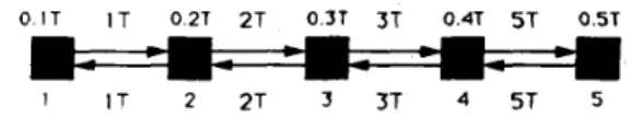
a simple example t o illustrate the timing of the local synchronization scheme based distributed computation. Figure 3 shows a 5-processor data communication network, and each processor is denoted by a black square marked below by a processor number. The communication delay of the data exchange in between the adjacent nodes are marked on the communication links, where T denotes a unit time. The elapsed time of the computation performed in each node processor in one iteration are marked on top of the node processor. For the sake of explanation, the communication delay and computation time in this example are arbitrarily assigned. However, the qualitative conclusions about synchronization derived from this example i s true for all combi- nations of computation time and communication delay. Now, to imitate the RQPD method based distributed computation, we make the following assumptions in the considered example. (1)

One iteration means that every node processor should perform its computation once and just once. (2) In every iteration, each node processor only needs data from adjacent nodes and itself to perform its computation. (3) In every iteration, each node starts computing after all the expected data are received. (4)

The computation process starts from time 0, a t which each node transmits the initial computed data to adjacent nodes. Figure

-4 shows four time frames of the procession of the local synchronization scheme based distributed computation of the considered example. The arrow marked by the processor number on top of the time scale indicates the instance that the processor receives all the expected data. Correspondingly, the instance that the processor finishes computation after receiving all the expected data is indicated by the arrow right below the time scale. From Figure 4, we see that the synchronization is already maintained

O . I T I T 0.2T 2 T 0.3T 3 T 0.41 5 T

n

0.5T

I'iqiire :). an example of data corimiuriication network

I 2 4.5 2 S I

I

I I I T 21 I T 47 O T I 2 3.1 I I _{5 4}₂ I t 1 I 1 61 77 I T 91 I OT I I I I I I0.W I I _5.4.2 I 1 4.5 2 I

1

I I 1 1 1 1641 ' I T L I T 1 4T 1 ST I t i . 2 I 3 5 4 2 I I I 1 I 17T I ET 1 OT 207 211 1 1 I I 2I.OT I I 5.4.2

Figure

4: procession of

the distributed

computation

in and after the second time frame (i.e., the second iteration). Moreover, the communication delay in one synchronized iteration is 5 T which is the maximum delay of a communication link in this example.

Global Termination Scheme: a two-phase global termination :scheme is employed here. T h e first phase is used t o determine

the convergence (or completion) of the quadratic subproblem. It ,checks whether max;{l&@(A)lm}

<

e. If yes, the second phase start t o check whether max,{Ik,lm}

<

to determine the com-

apletion of the distributed state estimation. In order t o carry out this two-phase global termination scheme in the data communication network, we need t o define a spanning tree of the data communication network and a special node designated as the root of the tree. A spanning tree of the network in Figure 2 is shown in Figure 5, where node 1 is the root node. A node is said t o be

a follower to node i if it is the head of a n arrow starting from a,

and we let F ( i ) denote the set of the followers to node i . Clearly, F ( i ) =

8

if i is a leaf node. A node is said t o be a predecessor of node i if i t is the tail of an arrow ending a t i. For example, F(4) = {2,3} and node 4 is the predecessor of nodes 2 and 3. We define the status of a node i , S,, as

(11) 1, if

I&q(A)lm

<

e and Sl = l , V 1 E F(k); 0, otherwise.

We also define the maximum observed deviation

l&lm

a t node i as

I~Y,I,

= max[I&Im,mpx

l&Im,

I E F ( ~ ) I (12)

Initially we assume that the status of all nodes are 0, which may change as computations proceed. The timing for any node processor i to transmit its S, and Idy,

Im

to its predecessor is when

St = 1 or S, just changed from 1 to 0. Any node processor i will

(5)

7’( C). conirniinical,ioii tiday of one data word transmission,

O( C ) : cominunication delay of global termination scheme.

Remark 7: We use T ( h , ) and T(H,,) because h, and H i j contain trigonometric functions, the computation of which can not be decomposed into the number of multiplications and additions.

The computation time including Communication delay of the distributed state estimator consists of two parts: (a) the recursive quadratic programming method in Steps 1-4 and Step 13 and ( b )

the dual method in Steps 5-12. Step 1 and 5 are initial guesses, thus no computation time is consumed.

Based on the defined notations, the computation time or the communication delay of the da.ta exchange corresponding to Step 2-12 that consumed in a node, say node il can be explicitly expressed in the following. Step 2 and 3 - 2T(C); Step4 -

T ( k )

+

T(Hit)

+

C ~ E ~ , [ T ( H ; I )

+

T(Hi,)]; Step 6 and 7 - 4T(C); Steps ~ [51hil

+

~ C I E J , Ih,lllT(x)

+

[~E,E.T, Ih,llT(+); Step 9

and 10 ~ 2T(C); Step 11 - [21h,l

+

2lJ,\lh,l]T(x)

+

[51h;l

+

21J,llh,l]T(+); Step 12 - Ih,lT(+). In the modified global ter-

mination scheme of Step 13, updat,ing 2; will take 2T( x ) + 2 T ( + ) computation time a t node i, however, the communication delay

O ( C ) 5 2tT(C)

+

tmax; IJlT(+). The upper bound of O(C) is

obtained based on the following facts (a) the computation time

of

“+”

and “compare” are about the same, and ( b ) the number of followers to any node i is less than max,

131,

In each step of Step 2-12 and the procedure of updating i i

in Step 13, the computations or the data exchange for all processors are carried out in parallel. Therefore, based on the local synchronization scheme, the computation time (or the communication delay) of the whole system in each of the above step is only ‘the maximum one of those consumed in all the individual nodes. For example, the computation time of the whole system in Step

4 is maxi{T(hi)

+

T ( H , , )

+

& - T ~ [ T ( H ; ~ )

+

T(Hli)]}. Thus, we may express the total computation time of the distributed state

r-t ima tor below:

I R . [ T ( R )

+

2 T ( C )

+

O ( C ) ]

+

I D . [ T ( D )

+

6T(C)] (13)

1 (ROOT)

J

5 ₂ ₍_FOLL~WER

TO NODE 4 )

F i g u r e 5: the s p a n n i n g t r e e of the n e t w o r k in Figurt. 2

update S, and Idy,(, according to (11) and (12) once SI and

I&llm

from all 1 E F ( i ) are received. Let t denote the number

of branches of the longest tree path from the root to a leaf in the spanning tree. If t,he status of the root, S, changes from

0 t,o 1 and remains 1 for consecutive f iterations of t,he dual method, then the current quadratic subproblem has completed t iterations before. When this occurs, the following decisions and the associated operations will be made at, the root node.

1) If

I&,lm

<

E , broadcasts a signal of completion of the state estimation problem to all nodes along tlie spanning tree.

2) If ldyrlm, 2 E , broadcasts a signal of updating 2 to all nodes, and each node i will return to Step 2 after it updates 2;.

Modification of the Global Termination Scheme: in order to determine the completion of the quadratic subproblem, updating the status S, a t each node i and broadcasting the result of the decision from the root node requires much communication over- head. Usually, the dual method improves fast for the first few tens of iterations but slows as it gets close to the solution. There- fore, we may set a maximum number of iterations, denoted by I t ,

that the dual method will iterate in solving the quadratic subproblem. Then, the first phase of the global termination scheme is modified by the directly updating 2, of each node i a t the end

of every I t iterations of the dual method. Then the second phase of the global termination scheme will be modified as follows:

After every Zt iterations of the dual method, the following procedures will be performed. Starting from the leaf nodes, each node i will update

18yi1m

according to (12) once it received all

l&,lm,I

E F ( i ) . Thereafter, it will transmit

(&,I,

to its predecessor. If the root node find ldy,l,

<

E after update, it will broadcast a signal of completion of estimation to all nodes.

Such modifications make the termination scheme simple, and also reduce the computat.ion time.

ANALYSIS O F COMPUTATION COMPLEXITY Following notations are used in this analysis:

I R : total number of the updates of 2,

I D : total number of the updates of A,

Ihll: the number of measurements 2,:

121:

the number of adjacent node processors of node i.

t : the number of branches of the longest tree path in the spanning tree,

T ( x ) : computation time for a multiplication,

T ( + ) : computation time for an addition or a subtraction,

T ( h i ) : computation time for the evaluation of h , ( z ) , T ( H ; j ) : computation time for the evaluation of d h , ( z ) / d z , ,

I t is w01 t h noting that the distributed state estimator has the nature of sparse-matrix technique. This property can be observed from the computation procedures of each node processor, in which each individual processor only needs data from adjacent nodes and itself t o carry out its computation. This indicates that only the operations involving nonzero terms are performed. Such nature of sparse-matrix technique is one of the causes that makes the computation complexity shown in (13)-(15) so simple.

Despite of the computation complexity obtained above, let

us compare the convergence rate of the RQPD method based distributed state estimator with tlie popular Newton method [2] based centralized state estimator. Newton method has quadratic convergence rate, however, at the expense of solving a large set of linear equations in each iteration. In the RQPD method, the recursive quadratic programming has superlinear convergence rate, and each quadratic subproblem is solved by the dual method which has linear convergence rate accompanied with the extremely simple calculations for each iteration as shown in (6), (7) and (9). From the above comparison, we see that the distributed state estimator will consume a lot more iterations than the centralized state estimator. However, the inherent properties of parallel computation and sparse-matrix technique of the distributed state estimator will achieve tremendous computation time saving as described by the simple computation complexity in (13)-( 15). A

(6)

I 3

556

strong support for this claim is manifested by simulations demonstrated in the section next to the following.

p

Along with the developed distributed state estimator, we can

obtain several attractive satellite functions. These functions are described or developed in the following.

(1) Reduction of the Time-Skew Problem centralized data acquisition.

The timeskew problem ie greatly reduced because of the de- ( 2 ) Topological Error Free Power Network Model

( 3 ) Easy Identification of the Unobservable States

It is true as we have explained in Remark 5 in previous section. The states xi of bus i can only be observed from its measure- ments r , or from the possible reiated measurements zt : { zip, zlq,

zltPr z l i q } , I E

3 .

zlv is excluded because it only has to do with ul, the voltage magnitude of bus 1. Based on this, the following simple procedures will be executed at each node i to identify the unobservable states.

Step idl: For each node 1 E

3,

send { z , ~ , z , ~ , z,lp, r,lp} to node 1. Step i d 2 If z, and q , for each 1 E

J,,

are all null, the states of this bus are unobservable.

Advantage of the above identification before estimating states is that we may add pseudo measurements for the unobservable states if necessary.

( 4 ) Jiad Data Detection and Identification

Although the decentralized data acquisition will have less communication noise in telemetry, the consideration of the bad data detection and identification is still necessary.

Bad

Data Detection Scheme- We employ the overall quadratic

cost function J(i) test [7] as our bad data detection scheme,

where J(i = [z

-

h ( i ) l T R - ' [ z

-

h(i) and i denotes the so- estimator.

By defining the node quadratic cost function J ( 2 , ) = [ z ,

-

h ( i , ) l T r ; ' [ r ,

-

h(i,)], we have J(i) = J ( i z ) . Based on the spanning tree (Figure 5 ) , we define j(i,) = J ( 2 , )

+EIEF(,)

j ( & ) . According to the above definition, we obtain j(ir) =

J(i).

Then the bad data detection scheme can be carried out along with the modified global termination scheme of the distributed state estimator as described below.

After every It iterations of the dual method, the following procedures will be performed. Starting from the leaf nodes, any nod: i will update its value of j ( 5 , ) once it receives all the values of J ( & ) , 1 E F(r). Moreover, each node i will send the value of j ( & ) to its predecessor once j(i,) is updated. Suppose theglobal termination criteria of the distributed state estimator,

l&lm

<

e,

is satisfied, the root node will compare J ( & ) with a preselected threshold value [Q to test the hypothesis of the existence of the bad data. If j(i,)

>

[Q, the root node will broadcast a command of starting bad data identification to all nodes along the spanning tree; otherwise, the estimation is complete.

Bad

Data Identification S c h e m e The weighted residual test will be employed here as our bad data identification scheme.

When receiving the command of starting bad data identification scheme, each node processor will compute the weighted residual

r y

= [rj

-

h , ( 2 ) ] / ~ ~ , of the associated measurement z j , where Q ~ , is the square root of the j-th diagonal element of R-'. Then each node processor will compare the magnitude of the computed weighted residual with a preselected threshold value [W. If IryI

>

[ w , this measurement will be treated as a suspected bad data. Consequently, each node processor will send the index and the magnitude of r," of the suspected bad measurement to the root node along the reverse direction of the spanning tree. The root node will then determine the largest one among all the received Iryl's, and broadcast the corresponding

index to all nodes. Meanwhile a re-estimation will start after the elimination of the bad data.

It is commonly known that the weighted residual test is less effective because the largest

1

is not necessarily corresponding 'to the bad measurement. However, a more sophisticated two- step residual test, which is as effective as but consuming less lution of t

b

e estimated states obtained

b

y the distributed state

computation time than the normalized residual test, is currently under development [12].

SIMULATIONS

In this section, we will demonstrate the computational performance of the distributed state estimator and its numerical accuracy by simulations.

Numerical Accuracy

We pick up three of our simulated cases on the IEEE 30-bus system for discussions. In these cases, we let the measurements be the real and reactive power line flows; the initial guess are from the flat-start; the parameters and constants are set below: e = 0.001, I t = 30, d = 0.01, = 1.50, R = I (the identity matrix), and y = 25. Then in the first case, we input the line flows from

a load flow solution of the 30-bus system as our measurements. The convergent result deviates from the load flow solution by

f0.0007p.u. in voltage magnitude and f0.004rad in phase angle

on the average. Such deviations are satisfactory and they will be smaller if L is chosen smaller. In the second case, we arbitrarily set

the states of a bus unobservable by discarding the data of line flows connected to bus 30 from previous set of measurements. The convergent result, excluding bus 30, of our distributed state estimator deyiates from the load flow solution by f0.0008p.u. in

voltage magnitude and f0.006rad in phase angle on the average. It is slightly less accurate than case 1 because less measurement information is supplied in this case. In the third case, we assume that the sign of the real power flows in two lines (lines 2-6 and 10-22) are mistakenly reversed. The convergent result deviates from that obtained by Newton method by f0.0003p.u. in voltage magnitude and f 0 . 0 0 2 r a d in phase angle. From the results of the above three cases, the numerical accuracy of the distributed state estimator are quite satisfactory.

Computationd PerfGrmance

The iterations of our distributed state estimator for the above three cases are ( I R = 27, I D = 810), ( I R = 24, I D = 7 2 0 ) and ( I R = 2 5 , I D = 7 5 0 ) respectively. The values I D = I R x f t

are large as we expect. Following is a comparison of the computational performance between the distributed state estimator and the Newton method based state estimator. We assume that the processing time of T ( x ) , T ( + ) , T ( h , ) and T(H,,) are the same in both methods, and compare their computation time first. T h e total computation time excluding the communication delay of the distributed state estimator includes two terms I R . T ( R ) and I D T ( D ) accordihg to ( 1 3 ) . On the other hand, the computation procedures in each iteration, say iteration

L,

of the Newton's method is t o set up the c o d c i e n t matrices H ( x k ) ( = [ a h ( x ) / a ~ ] l ~ = ~ t , ) , C(x')(= H ( Z ' ) ~ R - ' H ( ~ ' ) ) and the vector z - h ( s k ) first. Then it will solve the set of linear equations C ( x k ) A z k = r - h ( x k ) t o obtain Axk and updatezk+' = xk+Ask. -According to ( 1 4 ) - ( 1 5 ) and the simulation results, we find that

(a) the computation time I R . T ( R ) is approrimate to the elapsed time required to calculate the nonzero elements of H ( s o ) and

z

-

h(so), where xo is the initial guess of the states I, and (b) I D T ( D ) is about one tenth of (or comparable to) the computation time consumed in calculating the full matrix C ( x o ) (or the nonzero elements of C(zo)). Therefore, the total computa- tion time excluding communication delay in the proposed state estimator is just enough for the Newton's method to get ready to solve the set of linear equations in its first iteration. Fur- thermore, the total communication delay of the distributed state estimator is I R

.

[ 2 T ( C )

+

O ( C ) ]

+

6

.

I D

.

T ( C ) according t o ( 1 3 ) . Based on current optical fiber technologies, the data trans- mission speed ranges from 565 Mbits/sec [21] to 20 Gbit/sec [22]. For a data word of 32 bits, the total communication delay of our simulated cases is less than 0.3 ms, which is very small compared to the computation time. Therefore, our distributed state es- timator definitely outplay the Newton method in the aspect of computational performance.

CONCLUSION

We have developed a globally convergent distributed state es- timator which has several attractive satellite functions. Though we can not deny that when the system size grows, the iteration number of the distributed state estimator will be increasing at

(7)

551

least proportionally. However, the required computation t h e

is still small because of its inherent property of parallel coni- putation and the natriv of sparse-matrix technique. As we h a w demonstrated by simulations that the developed distributed state estimator has excellent computational performance.

It seems that the distributed state estimator is currently im- practical because the control technology of the power system is not yet reaching the status of decentralization, and the integra- tion of the data communication and power network is not yet matured. However, it is promising as pointed out by Gaushell and Darlington that we will be seeing the distributed processing throughout the utility's facilities in this decade [13]. Consider- ing the possibility of direct angle measurement in the future, the state estimation is still needed because bad data may be present. In that case, it is quite possible to develop a more simplified distributed state estimator than the one proposed.

Finally, we would like to point out that the distributed computation technique developed in this paper can be extended to solve the constrained nonlinear optimization problems of large- scale interconnected systems. Many power system management problems lie in this category. Therefore, we believe that our technique will not be limited t o state estimation.

ACKNOWLEDGMENT

This work was supported by National Science Council under Grant NSC79-0404-E009-48.

REFERENCES

[l] F. C. Schweppe and J. Wildes,"Power system static-state estimation, part I: exact model, " IEEE Trans. Power App..

Syst., vol. PAS-89, no. 1, pp. 120-125, Jan. 1970. [2] F. C. Schweppe,"Power system static-state estimation, part

111: implementation, IEEE Trans. Power App. Syst., vol. PAS-89, no. 1, pp. 130-135, Jan. 1970.

[3] A. Bose and K.A. Clements," Real-time modeling of power networks,"Proc. IEEE, vol. 75, no. 12, pp. 1607-1622, Dec. 1987.

[4] H. Kobayashi, S. Narita and M. S. A. A. Hamman,"Model coordination method applied to power system control and estimation problems," Proc. of the IFAC/IFIP 4th Int. Conf. on Digital Computer Appl. to Process Control, pp.. [5] H. Mukai," Parallel multiarea state estimation," Electric; Power Research Institute, report of research project 1764-, 1, Jan. 1982.

[6] Th. Van Cutsem and M. Ribbens-Pavella,"Critical survey' of hierarchical methods for state estimation of electric power systems,"IEEE Trans. Power A p p . Syst., vol. PAS-102, no. 10, Oct. 1983.

[7] L. Mili, Th. Van Cutsem and M. Ribbens-Pavella,"Bad data identification methods in power system state estimation - a comparative study,"IEEE Trans. Power App. Syst. vol. PAS-104, no. 11,pp. 3037-3049 Nov. 1985.

[8] M. Ikeda, D. D. Siljak and I<. Yasuda,"Optimality of de- centralized control for large-scale systems." Automaticu, 19, [9] Z. Shi and W. B. Gao, "Stabilization by decentralized don- trol for large-scale interconnected systems," Large-scale Sys- tems, 10,pp. 147-155 ,1986.

[lo] M. K. Sundareshan and R. M. Elbanna,"Large-scale systems with symmetrically interconnected subsystems: a.nal- ysis and synthesis of decentralized controllers," P roc. 29th

CDC, Honolulu, Hawaii! pp. 1137-1142, Dec. 1990. 114-128, 1974.

pp. 309-317, 1983.

[l I ] S.-Y. Lin,"A method to solve power system static-state estimation problem by using a network of processors," Proc. 29th C D C , Hawaii, Honolulu, pp. 3067-3072, Dec. 5-7, 1990.

[12] S.-Y. Lin, '' A distributed state estimator and bad data detection/identification of Power System, " NSC Report un-

der contract NSC79-0404-E009-48, Dept. of Control Eng., National Chiao Tung Univ., TAIWAN, ROC, Feb. 1991. [13] J. G. Dennis and T. D. Henry,"Supervisory control and

data acquisition,"Proc. IEEE, vol. 75, no. 12, Dec. 1987. [14] K. C. Holte,"Technology requirements for a competitive

electric utility market in the 21st century," IEEE Power Eng. Review, pp. 18-22, July 1989.

[15] J. Zaborszky, K. W. U'hang and K. V. Prasad,"Ultra fast state estimation for the large electric power system,"lEEE Trans. Automat. Contr., vol. AC-25,110.4 pp. 839-841, Aug. 1980.

[16] C. W. Brice and R. K. Cavin,"Multiprocesor static state estimation," IEEE Trans. Power App. Syst., vol. PAS-101, no. 2,pp. 302-308 Feb. 1982.

[17] D.G. Luenberger, Linear and nonlinear programming, sec- ond edition, MA: Addison-Wesley Publ. Co., 1984. [IS] S.P. Han," A globally convergent method for nonlinear pro-

gramming," Jounal of Optimization Theory and Applica- tions, vol. 22, no. 3, pp. 297-309, July 1977.

(191 A. S. Tanenbauni, Computer networks, N. J. Englewood Cliffs: Prentice Hall Inc.

,

1981.

[20] D.P. Bertsekas and J.N. Tsitstklis, Parallel and distributed computation, United Kingdom, London: Prentice Hall In- ternational Limited, 1989.

[21] M. Sotom et. al.,"Multichannel FSK transmission exper- iment a t 565 Mbits/s using tunable three-elect,rode DFB lasers," Electronics Letters, vol. 26, no. 13, pp. 869-870,: 21st June 1990.

[22] M. Nakazawa et. a1.,"20 Gbit/s solution transmission over 200 km using Erbium-doped fibre repeat,ers," Electianics

Letters, vol. 26, no. 19, pp. 1592-1593, 13th Sep:,1990.

Shin-Yeu Lin was born in Taiwan, ROC,

on June 26, 1953. He received the B.S.

degree in electronic engineering from Na- tional Chiao Tung University, the M.S. degree in electrical engineering from Univer- sity of Texas a t El Paso and the D.Sc. de-

gree in systems science and mathematics from Washington University in St. Louis, Missouri, in 1975, 1979 and 1983 respec- tivrly.

From 1984 t o 1985, he was with Wash- ington University working as a Research Associate then a Vis- iting Assistant Profew)r. From 1985 t o 1986, he joined G T E Laboratories working in the Switching Department as a Senior MTS. Since 1987 till now, he is an Associate Professor of Con- trol Engineering of National C h i m Tung University. His major research interests are Large-scale Power Systems, Optimization Theory and Applications, Distributed and Parallel Computa- tions.

!