The Impact of Information Technology on the
Banking Industry: Theory and Empirics
Shirley J. Ho
National Chengchi University, Taiwan
Sushanta K. Mallick
Queen Mary, University of London, UK
November 7, 2006
Abstract
This paper develops and tests a model to examine the effects of information tech-nology (IT) in the US banking industry. It is believed that IT can improve bank’s performance in two ways: IT can reduce operational cost (cost effect), and facilitate transactions among customers within the same network (network effect). The empir-ical studies, however, have shown inconsistency on this hypothesis; some agree with the Solow Paradox, some are against. Since most empirical studies have adopted the production function approach, it is difficult to identify which effect has dominated, hence the reasons attributed have been the difference in econometric methodology and measurement. This paper attempts to explain the inconsistency by stressing the heterogeneity in banking services; in a differentiated model with network effects, we characterize the conditions to identify these two effects and the conditions for the two seemingly positive effects to turn negative in the equilibrium. The results are tested on a panel of 68 US banks over 20 years, and we find that the bank profits decline due to adoption and diffusion of IT investment, reflecting negative network effects in this industry.
1
Introduction
The usage of information technology (IT), broadly referring to computers and peripheral equipment, has seen tremendous growth in service industries in the recent past. The most obvious example is perhaps the banking industry, where through the introduction of IT related products in internet banking, electronic payments, security investments, information exchanges (Berger, 2003), banks now can provide more diverse services to customers with less manpower. Seeing this pattern of growth, it seems obvious that IT can bring about equivalent contribution to profits.
In general, existing studies have concluded two positive effects regarding the relation between IT and banks’ performance. First, IT can reduce banks’ operational costs (the cost advantage). For example, internet helps banks to conduct standardized, low value-added transactions (e.g. bill payments, balance inquiries, account transfer) through the online channel, while focusing their resources into specialized, high-value added transactions (e.g. small business lending, personal trust services, investment banking) through branches. Sec-ond, IT can facilitate transactions among customers within the same network (the network effect) (see Farrell and Saloner, 1985; Katz and Shapiro, 1985; Economides and Salop, 1992). Let us consider the case of automated teller machines (ATMs) by banks. If ATMs are largely available over geographically dispersed areas, the benefit from using an ATM will increase since customers will be able to access their bank accounts from any geographic location they want. This would imply that the value of an ATM network increases with the number of available ATM locations, and the value of a bank’s network to a customer will be determined in part by the final network size of the bank. Indeed, Saloner and Shepard (1995), using data for United States commercial banks for the period 1971-1979, showed that the concern of network effect is important in the ATM adoption of United States commercial banks (see also Milne, 2006).
In view of these two effects above, it should be surprising to know that the evidence, however, shows some inconsistency in concluding the contribution of IT to banks’ profit.
Some studies echo the so called Solow Paradox in concluding that IT will actually decrease productivity. As stated by Solow (1987), "you can see the computer age everywhere these days, except in the productivity statistics". Shu and Strassmann (2005) studied 12 banks operating in the US for the period of 1989-1997 and found that although IT has been one of the most marginal productive factors among all inputs, it cannot increase banks’ profits. On the other hand, there are some studies agreeing with the positive influence of IT spending to business value. Kozak (2005) examines the impact of the progress in IT on the profit and cost efficiencies of the US banking sector during the period of 1992-2003. The research shows a positive correlation between the level of implemented IT and both profitability and cost savings.
The inconsistency in empirical results can be attributed to differences in measurement1 and econometric methodologies (Berger, 2003; Tam, 1998). Alternatively, the current paper attempts to provide an interpretation by stressing the heterogeneity in banking services. Indeed, compared to manufacturing industries or agriculture, banking industries present higher diversification in providing customer services. In this case, a differentiated model with network effects would probably describe the market better than the production function approach, which describes each bank’s profit (output) as a specific production function of inputs. Notice that most empirical studies2 have constructed their testing on productivity or growth. In addition, while most production approaches only present a mixture of IT influences on both demand and supply sides, a differentiated model can distinguish a network effect from the demand side (in banking services) from a cost reduction effect from the
1For example, Berger (2003) pointed out two approaches in measuring productivity: either by the
gov-ermment productivity indexes or by a modified form of the Solow (1957) neoclassical growth model (Oliner and Sichel, 2000).
2Computers may affect productivity because they are a specific capital input to the production process.
This is the approach taken in most existing studies, including both the national and industry-level studies just cited, as well as studies at the plant or firm level, such as Brynjolfsson and Hitt (2000), Dunne et al. (2000), Stolarick (1999), and McGuckin et al.(1998).
supply side. Most importantly, a differentiated model can characterize the competition in the industry, which cannot be distinguished from the cost effect in the production function approach.
Specifically, our paper examines the effect of IT in a modified Hotelling model with network effects due to Rohlfs (1974), and the theoretical conclusions are tested on a panel data of 68 US banks for the period 1986-2005. The keypoint to understand the inconsistency is to contemplate IT’s influence to the whole industry, rather than to the individual banks. For individual bank, it is true that both cost and network effects are positive. When all banks in the industry have the same access to this cost-saving technology, will the cost advantage from adopting IT vanish due to competition (in particular, price competition in banking industries). Will the presence of multiple networks bring determinative benefits to each bank in the industry? By investigating the equilibrium in a Hotelling model with network effects, we are able to explore the overall effect of IT to the whole industry.
The main findings are summarized as follows. First, we derive a simple test on the exis-tence of network effect by checking the relation between market share and IT expenditure. If there is only a cost reduction effect, each bank’s market share will increase with IT; how-ever, if there is also a network effect, the market share does not necessarily increase with IT. This result can be useful if a proxy variable for the size of network is invalid (Saloner and Shepard, 1995, use the number of branches possessed by a bank as a proxy for its expected ATM network size in equilibrium). Our test on the US banks shows that, the market share is positively related to IT expenditure indicating that there is a network effect.
Second, we are able to distinguish the cost reduction effect from the network effects. Since the equilibrium price will decrease with IT expenditure, if we could isolate this price effect by treating prices as one of the explanatory variables in the model, Proposition 2 shows that if the overall impact of IT on profits is negative, then the cost reduction effect is negative. Moreover, since in this case the market share still increases with IT, this negative result will indicate Berger’s (2003) observation that banks may have essentially "given away" the
benefits from the ATM technology in the 1980s as the industry became more competitive due to deregulation, and rents from market power shifted to consumers (p. 142). Our estimation of the US banks also show that if prices are treated as an explanatory variable, the overall impact of IT on profits is negative.
Finally, in line with both sides of the existing literature, we predict that banks’ profits can be positively or negatively related to IT expenditure. In the equilibrium, each bank’s price will decrease with its IT expenditure, but the impact on the profits will have to depend on whether its market share has increased. The overall effect on the whole industry, however, will depend on the relative sizes of weighted sum of IT and the average of IT. Here, the weight is measured by each bank’s profit share. For the data of US banks, we conclude that banks’ profits are negatively related to IT expenditure, showing that the weighted sum of IT in the US is less than the average of IT.
Overall, a differentiated model not only fits in the banking industry more, but also enables us to distinguish the network effect from demand side and the cost reduction effect from supply side. Our empirical study on the panel data of US banks shows that due to severe competition, each bank has over-invested in IT equipment, while the benefits from networks and cost reductions are competed away.
The remainder of the paper is organized as follows. Section 2 presents the modified Hotelling model with network effects and derives three results concerning the relation be-tween IT and equilibrium behaviors. In Section 3, the theoretical conclusions are tested on a panel data of 68 US banks for the period of 1986-2005. Section 4 concludes the paper.
2
The Model
To cope with the observation that banks provide highly differentiated products, we adopt a simple differentiated model (due to Hotelling, 1929) with two competitive banks and infinitely many heterogenous consumers. Some modifications are made to take into account
the network externality caused by the adoption of IT (see Rohlfs, 1974; Milne, 2006.). We will characterize the market equilibrium after the adoption of IT and derive three testable conclusions concerning the relation between market performance and IT expenditure.
To simplify, consider two competitive banks (A and B) in a banking industry, charging PA and PB respectively for services. There is a continuum of potential consumers indexed by x on the unit interval [0, 1] and let us assume that bank A is located at 0, while bank B is located at 1.
In addition to price competition, each bank invests ei, i = A, B, in IT equipment. For the individual bank, the adoption of IT has two effects: reducing the operational cost and creating a network effect to customer service. For the first effect, it is assumed that the adoption of IT will cut the operational cost from ci to ci
− ρ(ei), i = A, B; For the second effect, we follow Rohlfs (1974)’s setting in assuming that the valuation of service is positively related to the number of consumers in the same service. That is, let Vi(ei)denote the customers’ valuation for consuming bank i’s service and Vi(ei)is an increasing function of ei.
Each bank first determines its service charge (pi,i = A, B). After observing the service charges, each consumer then chooses the service according to her valuation on service, service charges and the preference difference between her and the bank that provides the service.
Consumers For an arbitrary consumer x, x ∈ [0, 1], the utilities for consuming each bank’s service is defined by (see also Shy, 1997):
Ux = nAVA(eA)− (x) − pA, if she uses bank A’s service; = nBVB(eB)− (1 − x) − pB, if she uses bank B’s service.
The valuation of service will depend on the size of IT equipment as well as the number of consumers (ni, i = A, B).
The negative terms −x and −(1 − x) indicate the preference difference between this consumer and bank A and B, respectively.
from bank A or B, i.e., nAVA(eA)
− (x) − pA = nBVB(eB)
− (1 − x) − pB. It can be easily checked that for consumers x <x,b they will choose bank A’s service; while for consumers x > b
x,service of bank B’s will be chosen. Hence, we know that nA=xband nB= 1
−bx.Replacing ni in the indifferent condition, we havexVb A(eA)− (bx)− pA= (1− bx)VB(eB)− (1 − bx)− pB, or alternatively bx = (1− V B(eB)) − (pA − pB) 2− (VA(eA) + VB(eB)) . (1) Notice thatbx(1 − bx) also denotes bank A’s (B) market share, given services charges and IT investments.
Profit Maximization of Banks Given each bank’s demand nA and nB, bank i, i = A, B, now chooses its service charge pi to maximize its profit πi, given by:
πA = (pA− (cA− ρ(eA)))((1− V B(eB)) − (pA − pB) 2− (VA(eA) + VB(eB)) )− e A, πB = (pB− (cB− ρ(eB)))((1− V A(eA)) + (pA − pB) 2− (VA(eA) + VB(eB)) )− e B. (2)
Notice that for our purpose of examining the impact of IT, we will treat IT as exogenous expenditures. The difference is that IT spending can reduce operational cost from ci to ci
− ρ(eA), and create an extra value to bank services.
Equilibrium The calculation of equilibrium is standard and hence will be omitted here. The equilibrium prices after adopting IT eiare pA=(3−2VB(eB)−VA(eA))+2(cA−ρ(eA))+(cB−ρ(eB))
3
and pB=(3−VB(eB)−2VA(eA))+(cA−ρ(eA))+2(cB−ρ(eB))
3 .In particular, the price difference
pA− pB = (V A(eA) − VB(eB)) + (cA − ρ(eA)) − (cB − ρ(eB)) 3 . (3)
Moreover, the equilibrium demand for bank A is nA=(1−VB(eB))−(V A(eA)−VB (eB ))+(cA−ρ(eA))−(cB−ρ(eB))3
2−(VA(eA)+VB(eB)) ,
and the demand for bank B can be derived similarly. Finally, the equilibrium profits after the adoption of IT are πA= ((3−2VB(eB)−VA(eA))+2(cA−ρ(eA))+(cB−ρ(eB))
3 )
3−VA(eA)−2VB(eB)
6−3(VA(eA)+VB(eB))−eA,
and πB= ((3−VB(eB)−2VA(eA))+(cA−ρ(eA))+2(cB−ρ(eB))
3 )
3−2VA(eA)−VB(eB)
Main Results Here we derive three testable results concerning the impact of IT. Proposition 1 helps us to examine the existence of network effect through checking the relation between market share and IT.
Proposition 1 (i) If IT has only a cost reduction effect, then bank i’s equilibrium price will decrease with ei and market share increases with ei; (ii) If IT has also a network effect, then bank i’s equilibrium price also decreases with ei but the market share will increase or decrease with ei.
Proof. (i) If IT has only a cost reduction effect, Vi is not affected by ei.The partial differ-entiation of equilibrium price w.r.t. ei will be −23 ρ0(ei).Moreover, the partial differentiation of market share (see bx in (1)) w.r.t. ei will be negatively related to the differentiation of pA
− pB, which according to (2) is negatively related to ei. Hence, market share must in-crease with IT expenditure. (ii) If IT has also a network effect, Vi is affected by ei. The partial differentiation of equilibrium price w.r.t. ei will be −V0(ei)−2ρ0(ei)
3 . Moreover, since pA
− pB can be negatively related to ei, the partial differentiation of market share (see bx in (1)) w.r.t. ei is not necessarily positive. Hence the market share does not necessarily increase with ei.
The significance of Proposition 1 is to provide a first step check on the existence of network effect. If the relation between market share and IT is negative, then it implies that there exists a network effect; but if the relation is positive, nothing conclusive can be told about the existence of network effects. This result can be useful if a proxy variable for the size of network is invalid.
The existence of network effects is not enough to judge the overall impacts of IT. The overall impact is a combination of effects on prices, cost and market share (demand). How-ever, we are able to distinguish the cost reduction effect from the network effects. Proposition 1 describes that the equilibrium price will decrease with IT expenditure. If we could isolate this price effect by treating prices as one of the explanatory variables in profit regression,
the effects will be limited on cost and market share. Since in this case market share still in-creases with IT, and if the relation between profits and IT is negative, then we can conclude that the cost reduction effect is negative.
Proposition 2 If the impact on prices are isolated, then (i) the market share is increasing in ei; (ii) if IT has negative effect on profits, then the network competition effect is higher than the cost reduction effect.
Proof. Given pAand pB as exogenous, (i) the partial differentiation of bx in (1) with respect to ei is VA0(eA)((1−VB(eB))−(pA−pB))
[2−(VA(eA)+VB(eB))]2 , which is positive; (ii) Since xb is positively related to ei,
it is easy to see from the definition of πi that if IT has negative effect on profits, then the network competition via price effect is higher than the cost reduction effect.
Finally, in line with both sides of the existing literature, we predict that banks’ profits can be positively or negatively related to IT expenditure. The overall impact consists of effects on prices, cost and market share (demand). For the individual bank, Proposition 1 has shown that equilibrium prices will decrease with IT. Next, the cost effect is a combination of two parts: IT expenditure as cost, and the reduction of operational cost due to IT. This term could be positively or negatively related to IT, depending on whether the reduction on the operational cost is competed away in the market competition. Lastly, we have proved in Proposition 2 that if the price effect is isolated, IT has positive impact on market share. However, since equilibrium price will be decreasing in IT, through the definition in (1), there is no conclusive result concerning the effect on market share.
Moreover, although the valuation of consumer service will change with IT, the total size of consumers is fixed (i.e., restricted to the unit interval). If one bank’s market share increases with IT, the other bank’s market share cannot increase simultaneously. Since the empirical tests are examined with bank level data, it is useful to recall from the basic econometric text about the sign for the parameter of IT in the regression. That is, if we run the regression of profits (πi) on IT expenditures (ei), the sign for the parameter of IT
will depend on whether X(πi − πi)(ei − ei) ≷ 0, where πi = Pπi n and ei = Pei n. After rearranging, this condition becomes
X πi P
πiei− X ei
n ≷ 0. (4)
Here n denotes the number of banks in the industry. In other words, the overall effect on the whole industry will depend on whether IT can change the relative sizes of weighted sum of IT and the average of IT. If there are scale economies in adopting IT, then the sign in (4) will be positive. Berger (2003) observed that in the US, although large banks have significant scale economies associated with back-office operations (cost reduction), small firms are often able to share in the benefits of technological progress (network effect). The overall impact on profits is therefore ambiguous.
3
Empirical Study
The purpose of empirical study is to see how the differentiated model above can help us understand the overall impact of IT on commercial banks in the US. The data consists of a panel of 68 US banks for the period 1986-2005. Since most existing research on US banks has adopted the production function approach (see Shu and Strassmann, 2005, for a review), it is not easy to distinguish the network effect from the demand side and the cost reduction effect from the supply side, or to characterize the effect from competition in this highly diversified industry. Our theoretical discussion above directs us three steps to unravel the overall impacts.
First, we can check the existence of network effect by examining the relation between market share and IT. According to Proposition 1, we will test the following empirical models, where the subscripts denote time t for the period 1986-2005.
pit = α0+ αITti+ ε i t, xit = β0+ βITti+ εit,
where pi
t, ITti and xit denote bank i’s prices, IT expenditures and market shares at time t. Notice that we have replaced ei
t with ITti to make a clear distinction from the error term εit. The first equation provides a preliminary check if the data can fit the differentiated model, where αi is expected to be negative. The second equation tests if there is a network effect: if β is negative, then there is a network effect, but if β is positive, then nothing conclusive can be said about the existence.
Second, in order to distinguish the cost reduction effect from the network effects, we iso-late the price effect by treating prices as one of the explanatory variables in profit regression, and test the following model
πti = δ0+ δpit+ γITti+ ηWti+ εit. where Wi
t denotes bank i’s wage expenditures at time t. If γ is negative, then following Proposition 2, we can conclude that the cost reduction effect is negative.
Third, we test the overall impacts of IT on profits, by testing the following model, having only controlled for the effect of wage cost
πit= σ0+ λITti + φW i t + ε
i t.
If λ is negative, then the overall impact (cost reduction effect and network effect) of IT is negative; If λ is positive, then the overall impact of IT is positive.
3.1
Data Source and Discussion
Variables have been extracted from Company Accounts in the Worldscope database from Datastream. The definitions are given as follows.
πi
t: net revenues represent the total operating revenue of the company. ITi
t : IT expenditure represents equipment expenses by banks, excluding depreciation cost.
xi
t:market share is calculated as the share of each bank’s revenue over the total revenue of the banking industry (in this case 68).
pi
t : average prices are calculated as interest expense over net revenue. Interest expense represents the total amount of interest paid by the bank.
Wi
t :staff or labour cost, which includes wages and benefits paid to employees and officers of the company.
Oi
t : other operating expenses have been used as a possible instrument in the 2-stage GLS.
As the above variables are collected from one single database, an important methodolog-ical issue relating to data comparability that normally arises with IT data has been resolved. As is well known, the US banking industry has undergone major structural changes with frequent mergers and acquisitions and, consequently, all banks do not have extensive his-torical expenditure data. Therefore, our sample only covers 68 banks which have data for a relatively longer time period that allows us to carry out a dynamic analysis. The banks in our sample have an average of $2197 billion in terms of revenues and $72 billion in terms of average equipment investment. Shu and Strassman (2005) discuss several problems as-sociated with IT related data either from the US Bureau of Economic Analysis or other government agencies. Thus, researchers have used different sets of IT spending data, for example, the data from the International Data Group (IGD) survey on about 300 com-panies. But, the reliability of such a data set is still questionable because it used mail-in questionnaires or telephone surveys which are either incomplete or from interpretations that deal more with the views of the respondents than the facts. We chose the banking industry because it is part of the service industry that has been suspected of having one of the lowest IT productivity, as in Shu and Strassman (2005). Thus, the objective of this paper is to analyze the banking industry using bank-level data on equipment expense with reasonably long time dimension as a suitable proxy for IT spending.
3.2
Empirical Results
The aim is to investigate whether IT investments improve banks’ profitability. Based on the above framework, we estimate the contribution of firm-level equipment investment in IT to the financial performance of banks. The cross-sectional and time series nature of the available data (68 banks for a time period of 20 years) allows us to make use of a sufficiently broad sample dimension, giving a pooled total sample of 1293 observations. The parameters that are to be estimated are assumed to be constant across banks and over time, as it is common with a regression model. Except market share and average price (which are expressed in terms of ratios), all other variables are measured in logarithms to adjust for heteroskedasticity; thus the coefficients measure the elasticity of prices, market shares and profits.
We run different methods of estimation for checking robustness of the parameters. Two-stage Generalised Least Squares (GLS) (with fixed and random effects) and Generalised Method of Moments (GMM) procedures have been used. There are no significant differences between the parameters estimated with these various techniques, denoting the robustness of our estimates. The advantage of the 2-stage GLS method is that it corrects for the condition of heteroschedasticity. GMM, on the other hand, is more appropriate for obtaining efficient estimates, correcting for heteroscedastic errors and considering a dynamic model. To capture possible dynamics, we have added relevant lagged dependent variables in each of the three equations. The overall performance of panel estimates is satisfactory. The relationships between the dependent variables and the independent variables in the three different models are strong, with the t-values significant at a 1% level in each model. The values obtained for R2 is satisfactory, as they are fairly high. The 2-stage GLS and GMM estimation results for prices and market share appear in Table 1, whereas Table 2 presents results drawing inferences for bank profits, uncovering network effects and the role of competition.
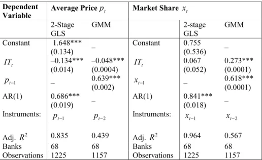
Table 1: Panel Regressions for Average price (pt) and Market shares (xt) Dependent
Variable Average Pricept Market Share xt
2-Stage GLS GMM 2-stage GLS GMM Constant 1.648*** (0.134) – Constant 0.755 (0.536) – t IT –0.134*** (0.014) –0.048*** (0.0004) ITt 0.067 (0.052) 0.273*** (0.0001) 1 − t p – 0.639*** (0.002) xt−1 – 0.618*** (0.0001) AR(1) 0.686*** (0.019) – AR(1) 0.841*** (0.018) – Instruments: pt−1 pt−2 Instruments: xt−1 xt−2 Adj. R2 0.835 0.439 Adj. R2 0.964 0.567 Banks 68 68 Banks 68 68 Observations 1225 1157 Observations 1225 1157 Notes: figures in parentheses are standard errors; *, ** and *** indicate a significance level at the 10%, 5% and 1% level respectively. Panel bank-specific fixed effect. GLS – Generalized Least Squares, GMM – Generalized Method of Moments dynamic panel. IT variable is expressed in logs.
It is apparent from results in Table 1 that average prices are negatively related to IT spending, whereas market share is insignificantly related to the IT spending in the 2-stage GLS, but in the GMM estimation it turns out to be positively significant in influencing market share. In other words, one could conclude that the market share could either increase or remain unchanged. The latter is likely to reflect the case of a network effect. In Table 2, we present the revenue effects of IT spending, after having controlled for the effects of average price and salary cost. We find consistently a negative effect of IT on revenue and the result is robust across different methods of estimation (see Table 2A). The model is formulated with other operating expenditure along with the lagged dependent variables as instruments to correct for any endogeneity bias.
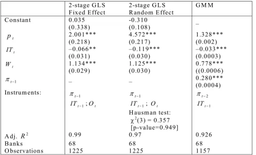
As we need to distinguish network effect from the cost reduction effect, we have omitted average price as a regressor from the profit regression and estimated the effect of IT on bank profits (see Table 2B). The estimates reported in Table 2B further support the robustness of our estimates. In all cases the coefficients remain significantly different from zero. The negative effect of IT on profit still holds, although in the dynamic panel regression (GMM),
the sign turns marginally positive indicating that the network effect is relatively small, in the sense that some banks benefit from more customers; while others are actually losing their customers. In this case, the profit from cost reduction is marginally more than the loss from the negative network effect, as the magnitude of the coefficient is very small. Thus the overall effect of IT on revenue here turns positive.
Table 2A: Panel Regressions for Bank Profits (πt)
2-stage G LS Fixed Effect 2-stage G LS Random Effect G M M Constant 0.035 (0.338) -0.310 (0.108) – t p 2.001*** (0.218) 4.572*** (0.217) 1.328*** (0.002) t IT –0.066** (0.031) –0.119*** (0.030) –0.033*** (0.0003) t W 1.134*** (0.029) 1.125*** (0.030) 0.778*** ((0.0006) 1 − t π – – 0.280*** (0.0004) Instrum ents: πt−1 πt−1 πt−2 1 − t IT ;Ot ITt−1; Ot ITt−1 H ausman test: χ2(3) = 0.357 [p-value=0.949] A dj. R2 0.99 0.97 0.926 Banks 68 68 68 O bservations 1225 1225 1157
N otes: Standard errors are in parentheses. *, ** and *** indicate a significance level at the 10% , 5% and 1% level respectively. Panel bank-specific fixed effect. ITt, πt, Wt, and Ot have been used in logs.
Table 2B: Panel Regressions for Bank Profits (πt)
2-stage GLS Fixed Effect 2-stage GLS Random Effect GM M Constant 2.487*** (0.284) 0.409*** (0.143) – t IT –0.337*** (0.075) –0.598*** (0.061) 0.005*** (0.0003) t W 1.210*** (0.078) 1.612*** (0.063) 0.312*** (0.0001) 1 − t π – – 0.598*** (0.0001) Instruments: πt−1 πt−1 πt−2 1 − t IT ITt−1 ITt−1 Hausman test: χ2(2) = 3.019 [p-value=0.221] Adj. R2 0.982 0.933 0.901 Banks 68 68 68 Observations 1225 1225 1157
Notes: Standard errors are in parentheses. *** indicates significance at 1% level. Panel bank-specific fixed effect and period-specific random effect. ITt,πt, and Wt have been used in logs.
Our results are consistent with the testable implications of the theoretical propositions derived in the previous section:
(1) There exists a negative relation between IT investment and price levels.
(2) Market share increases with higher levels of IT, although the result is significant with a GMM model.
(3) Prices contribute positively to firm profitability.
(4) Banks with higher levels of IT have lower profitability due to the possibility of network effect, and the impact turns out to be marginally positive in a dynamic context, if price as a control variable is not considered.
This study contributes to the understanding of how IT contributes to the banking indus-try in the US or the service indusindus-try in general. Prior research has linked IT to productivity, while this research provides evidence that IT is also related to profitability. Our results are also consistent with prior assertions that IT-innovations could create network effects but that may not be easily captured in the productivity approach adopted in previous studies. Thus our results do lend evidence that IT can have a negative effect on profitability and the consistency across different methods of estimation gives us greater confidence in our results.
4
Conclusion
This paper is concerned with the impact of information technology on the banking industry, as banks are the intensive users of IT. The usage of IT can lead to lower costs, but the effect on profitability remains inconclusive owing to the possibility of network effects that arise as a result of competition in financial services. The paper analyzes both theoretically and empirically how information technology related spending can affect bank profits via competition in financial services that are offered by the banks. The paper utilizes a Hotelling model to examine the differential effects of the information technology (IT) in moderating the relationship between costs and revenue. The impact of IT on profitability is estimated
using a panel of 68 US banks over 20 years. Both static and dynamic panel econometric techniques are utilized to examine the differential impact of IT on average prices, market share and profits. The results document the role of IT on the cost and revenue in banking and show the impact of network effects on bank profitability. While IT might lead to cost saving, we show that higher IT spending can also create network effects lowering bank profits. Besides, IT spending has a positive effect on market share.
The relationship between IT expenditures and bank’s financial performance or market share is conditional upon the extent of network effect. If the network effect is too low, IT expenditures are likely to (1) reduce payroll expenses, (2) increase market share, and (3) increase revenue and profit. The evidence however suggests that the network effect is relatively high in the US banking industry, implying that although banks use IT to improve competitive advantage, the net effect is not as positive as normally expected. In a broader context, the innovation in information technology, deregulation and globalisation in the banking industry could reduce the income streams of banks, and thus the strategic responses of the banks, particularly the trend towards mega-mergers and internal cost-cutting, are likely to change the dynamics of the banking industry. Given our negative result due to possible network effect, the changing banking environment could still make it insufficient to offset any reduction in income.
References
Berger, A. N. (2003), The economic effects of technological progress: evidence from the banking industry, Journal of Money, Credit, Banking, 35 (2), 141-176.
Brynjolfsson, E., and Hitt, L.M. (2000), Beyond computation: information technology, organizational transformation and business performance,” Journal of Economic Perspec-tives, 14(4), 23-48.
dispersion in U.S. manufacturing: the role of computer investment, NBER Working Paper 7465.
Economides, N. and Salop, S. (1992), Competition and integration among complements, and network market structure, The Journal of Industrial Economics, XL (1), 105-123.
Farrell, J. and Saloner, G. (1985), Standardization, compatibility and innovation, RAND Journal of Economics, 16 (1), 70-83.
Hotelling, H. (1929), Stability in competition, Economic Journal, 39, 41—57.
Katz, M. and Shapiro, C. (1985), Network externalities, competition, and compatibility, The American Economic Review, 75 (3), 424-440.
Kozak, S. (2005), The role of information technology in the profit and cost efficiency im-provements of the banking sector, Journal of Academy of Business and Economics, February 1, 2005.
McGuckin, R. H., Streitwieser, M. and Doms, M. (1998), The effect of technology use on productivity growth, Economic Innovation and New Technology, 1—26.
Milne, A. (2006), What is in it for us? Network effects and bank payment innovation, Journal of Banking & Finance, 30 (6): 1613-1630.
Oliner, S. and Sichel, D. (2000). The Resurgence of growth in the late 1990s: Is infor-mation technology the story?, Journal of Economic Perspectives 14, 3-22.
Rohlfs, J. (1974), A theory of interdependent demand for a communication service, Bell Journal of Economics, 5 (1), 16-37.
Saloner, G. and Shepard, S. (1995), Adoption of technologies with network effects: an empirical examination of the adoption of automated teller machines, RAND Journal of Economics, 26(3), 479-501.
Shu, W. and Strassmann,P. A. (2005), Does information technology provide banks with profit?, Information and Management, 42 (5), 781-787.
Stolarick K. M. (1999), Are some firms better at IT? Differing relationships between productivity and IT spending, Working Paper CES99-13, U.S. Census Bureau, 1999.
Shy, O. (1997), Industrial Organization: Theory and Practice, The MIT Press. Solow, R. (1987), We’d better watch out, New York Times Book Review, July 12. Solow, R. (1957), Technical Change and the Aggregate Production Function, Review of Economics and Statistics, 39: 312-320.
Tam, K. Y. (1998), The impact of information technology investments on firm perfor-mance and evaluation; evidence from newly industrialized economies, Information System Research, 9 (1): 85-98.