通大學]
On: 28 April 2014, At: 02:14 Publisher: Taylor & Francis
Informa Ltd Registered in England and Wales Registered Number: 1072954 Registered office: Mortimer House, 37-41 Mortimer Street, London W1T 3JH, UK
International Journal of
Production Research
Publication details, including instructions for authors and subscription information:
http://www.tandfonline.com/loi/tprs20
Mixing macro and micro
flowtime estimation model:
Wafer fab example
T.-Y. Tseng , T.-F. Ho & R.-K. Li Published online: 14 Nov 2010.
To cite this article: T.-Y. Tseng , T.-F. Ho & R.-K. Li (1999) Mixing macro and micro flowtime estimation model: Wafer fab example, International Journal of Production Research, 37:11, 2447-2461, DOI: 10.1080/002075499190608
To link to this article: http://dx.doi.org/10.1080/002075499190608
PLEASE SCROLL DOWN FOR ARTICLE
Taylor & Francis makes every effort to ensure the accuracy of all the information (the “Content”) contained in the publications on our platform. However, Taylor & Francis, our agents, and our licensors make no representations or warranties whatsoever as to the accuracy, completeness, or suitability for any purpose of the Content. Any opinions and views expressed in this publication are the opinions and views of the authors, and are not the views of or endorsed by Taylor & Francis. The accuracy of the Content should not be relied upon and should be independently verified with primary sources of information. Taylor and Francis shall not be liable for any losses, actions, claims, proceedings, demands, costs, expenses, damages, and other liabilities whatsoever or howsoever caused arising directly or indirectly in
connection with, in relation to or arising out of the use of the Content. This article may be used for research, teaching, and private study purposes. Any substantial or systematic reproduction, redistribution,
and use can be found at http://www.tandfonline.com/page/terms-and-conditions
Mixing macro and micro ¯ owtime estimation model: wafer fab example
T.-Y. TSENG² , T.-F. HO² and R.-K. LI² *Accurately predicting the order ¯ owtime for a wafer fab is a critical task. Previous investigations involving ¯ owtime estimation of the regression approach have extensively applied the macro ¯ owtime estimation concept. The `macro’ ¯ owtime estimation concept constructs only one aggregate model to estimate the ¯ owtime as a whole. In contrast, the `micro’ ¯ owtime estimation approach constructs an individual regression model for each stage of operation to estimate its individual ¯ owtime. The cumulative order estimated ¯ owtime is then the sum of the indi-vidual estimated operation ¯ owtime. Each approach has its own merits and lim-itations. Therefore, in this study we examine the feasibility of mixing the macro and micro ¯ owtime estimation models. Comparing the proposed model with a variety of macro and micro models reveals that the mixed macro and micro ¯ owtime estimation model can achieve a balance between ¯ owtime estimation error and model complexity.
1. Introduction
Accurately predicting the order ¯ owtime for a wafer fab is a critical task. Typical applications include assigning due-dates for customers, planning the order release, and evaluating the performance of scheduling policies for any unforeseen disturb-ances. Calculating the order ¯ owtime allowance is not straightforward owing to the dynamic nature of wafer fab, in which new wafers are constantly arriving and order priorities are constantly changing. Although developing a system capable of always accurately predicting order ¯ owtime is impossible, a relatively simple yet accurate method is highly desired.
The order ¯ owtime is based on the processing time of operations and the order interoperation time, which consists of queue time, move time and waiting time. The queue delays are caused by resource contention due to factors such as machine status, variability in processing times, variability in arrival times, and variability in batch sizes. Investigations involving ¯ owtime estimation have generally applied four di erent approaches. The ® rst is the simulation approach (Weeks and Fryer 1977, Weeks 1979, Bertrand 1983, Baker 1984, Srivatsan and Kemf 1995, Lawrence 1995). By using current orders on shop and shop loads to simulate forward in time, the simulation is extremely general and can model nearly any conceivable production system; however, it is computationally expensive and time consuming (Connors et al. 1996).
The second approach is analytical research such as the queueing model. Previous works involving analytical models (Heard 1976, Seidmann and Smith 1981, Cheng
International Journal of Production Research ISSN 0020± 7543 print/ISSN 1366± 588X on lineÑ 1999 Taylor & Francis Ltd http://www.tandf.co.uk/JNLS/prs.htm
http://www.taylorandfrancis.com/JNLS/prs.htm
Revision received August 1998.
² Department of Industrial Engineering and Management, National Chiao Tung University, 1001 Ta Hsueh Road, Hsinchu, Taiwan 30050.
³ To whom correspondence should be addressed.
and Gupta 1989, Bookbinder and Noor 1985, Karmarkar 1987, Wein 1991, Lynes and Miltenburg 1994, Enns 1995, Connors et al. 1996) have elucidated problems that limit their practices. For example, they are valid only for a ® rst-come, ® rst-served (FCFS) dispatch rule. However, in practice, the FCFS is not generally recognized as the optimal one. Another problem is that the shop ¯ oor must be in a steady state, which is impossible in nearly every job shop (Baudin et al. 1992).
The third approach is the neural network model. By using historical data as the input variables, the neural network can capture the previous pattern of the system and predict on the basis of future events. Although a few cases have been imple-mented in manufacturing (Udo 1992, Philipoon and Fry 1992, Zhang and Huang 1995), the unknown process engine of a neural network increases the suspicion and unwillingness to accept in most practitioners.
The fourth approach is the regression model. By using historical data similar to how a neural network functions, the regression model di ers from a neural network only in that the former appears to be more reasonable than the latter from the statistical perspective. Earlier works on ¯ owtime estimation such as CON, RDM, TWK, NOP, JIQ (Eilon and Chowdhury 1976), JIS (Week 1979), OFS (Vig and Dooley 1991), and COFS (Vig and Dooley 1993) belong to this approach. However, these heuristic models can be viewed as ¯ owtime prediction models only if regression analysis is used to determine the parameters.
Although numerous regression related heuristics have been developed and tested for estimating the ¯ owtime or due-date (with some of these apparently quite e ec-tive), these rules have still not been fully developed owing to two features: the linear independence of explanatory variables and a macro view. The linear independent assumption prevents more explanatory variables to join the regression model because the mutually independent explanatory variables are rare in reality. Consequently, a trade-o arises between easy explanation and better ® tting regard-less of whether or not more dependent variables are involved. Therefore, the relative importance of the explanatory variables and their in¯ uence on the ¯ owtime deter-mination must be systematically investigated to minimize the prediction error. Stepwise regression is commonly used to identify the following: (1) the important variables in the ¯ owtime estimation, (2) the interaction e ects between the input variables, (3) the optimal form of explanatory variables and (4) the coe cients of estimation equation.
With the regression prediction approach, either the macro or micro ¯ owtime estimation concept can be applied. The `macro’ ¯ owtime estimation concept con-structs only an aggregate regression model to estimate the ¯ owtime as a whole. Its explanatory variables are total processing time, total number of jobs, or total number of operations. This concept prevails in conventional regression ¯ owtime estimation approaches. However, in a wafer fab, over 100 operational stages are common, and each operational stage may have unique features. The coe cients of the regression ¯ owtime estimation model for each operation may be not equivalent statistically; and then the forecasting error with the macro ¯ owtime estimation approach may be too large to be acceptable. Thus, the validity of the macro concept is questionable. A `micro’ ¯ owtime estimation approach, unlike a macro view, con-structs an individual regression model for each operation stage to estimate its indi-vidual operational stage ¯ owtime. Assume that only interaction e ects among explanatory variables of the same stage are included, and that those of di erent stages are less signi® cant and are thus neglected. Then the total order estimated
¯ owtime equals the sum of the individual estimated operation ¯ owtime. An illus-trative example presented here demonstrates that properly selecting the explanatory variables can reduce the interaction e ects between operation stages.
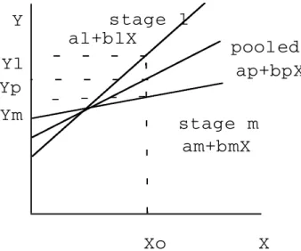
Chatterjee and Price (1991) analysed a situation in which a regression equation for a pooled data set can represent separated regression equations for subsets of the data collected. A serious bias may be incurred if one regression relationship is used to represent the pooled data set. Figure 1 depicts two ¯ owtime estimation models: macro and micro models. Let Y represent the ¯ owtime and let X be work in process (WIP). In the macro model, the operational stage distinction is ignored, the data are pooled and only one line exists. However, in the micro model two separate regression lines are available for the both operational stages, l and m, each with distinct regres-sion coe cients. The graph indicates that if Xland Xmhave been set at certain levels
of WIP for operational stages l and m respectively, by using the macro model, the total expected ¯ owtime is ap+bp
(
Xl+Xm)
when total WIP on the shop is Xl+Xm.However, if the micro model is selected, the actual ¯ owtime estimates are Yl
(
=
al+blXl)
for stages l and Ym(
=
am+bmXm)
for stage m when the individualstages WIP are Xl and Xm. Substituting
(
ap+bp(
Xi+Xm))
for(
al+am+blXl+bmXm)
represents a bias for stages l and m. Whether the macroor micro model is used depends on if
(
ap+bp(
Xl+Xm))
is within a certain level ofcon® dence intervals of
(
al+am+blXl+bmXm)
.Owing to the unavoidable bias incurred for the macro ¯ owtime estimation from pooled data (Chatterjee and Price), predicting micro ¯ owtime estimation is more accurate than estimating the macro ¯ owtime. Although the micro concept reduces the forecasting error, the complexity of the estimation model is too high. This model is too di cult to implement in practice, particularly in a wafer fab, where over 100 operational stages are common. Therefore, in this study we examine the feasibility of mixing the macro and micro ¯ owtime estimation models. The proposed model initi-ally applies the micro approach to construct an individual regression equation for each operation stage. A macro approach is then used to group together those
opera-Y
Yl
Yp
Ym
stage l
pooled
stage m
X
Xo
al+blX
am+bmX
ap+bpX
Figure 1. Pooled and distinct regression.
tional stage regression equations that have the same combination of explanatory variables but with di erent coe cients. A macro ¯ owtime estimation equation is then ® tted for those clustered operation stages. The criterion of whether those opera-tion stages can be ® tted into a macro regression equaopera-tion is based on its predicopera-tion error. The mixed macro and micro ¯ owtime estimation model is constructed and updated on the basis of the samples of the recently completed orders. Next, the total ¯ owtime through all operational stages is estimated by merely summing the value of explanatory variables of each stage into the corresponding grouped macro equations instead of summing individual stage ¯ owtimes estimated by micro equations. Thus, a balance can be achieved between ¯ owtime estimation error and model complexity. In addition, the proposed model is also compared with various macro and micro ¯ ow-time estimation models in terms of factors such as mean absolute deviation, mean square error, mean absolute percent error, number of tardy jobs, percent of tardy jobs, average lateness, and standard deviation of lateness.
2. Fundamental concept and algorithm for the mixed macro and micro ¯ owtime estimation model
Assume that a set of data consists of K explanatory variables, X1,X2,. . .,Xk,
which may include interaction e ects among input variables of the same operation stage and P operational stages, then the macro and micro ¯ owtime estimations through the whole stages areY andª Y , respectively:ª
ª Y
=
b 0+b 1X1+ +b KXK ª Y=
P i=1 ª Y=
P i=1(
b i0+b i1Xi1+ +b iKXiK)
.(
1)
The coe cients of the macro equation,(
b 0,b 1,. . .,b K)
, are recalculated from pooleddata of P operation stages. If one macro ¯ owtime estimation can replace P micro ¯ owtime estimation equations, then the micro approach total ¯ owtime estimationYª can be replaced by the macro approach ¯ owtime estimation Y which is simplyª calculated by summing the explanatory variables of P operation stages into the macro equation, where
X1
=
P i=1 Xi1,. . .,XK=
P i=1 XiK.Since the micro ¯ owtime estimation model ® ts the shop well and the total ¯ owtime estimation used in the micro ¯ owtime estimation model is equal to the summation of the ¯ ow time estimation of each individual operation stage, no bias variance is incurred. Therefore, the sum of square error (SSE) for micro ¯ owtime estimation is lower and the complexity is higher than that for macro ¯ owtime estimation. On the other hand, the SSE for the macro ¯ owtime estimation is in the upper bound and the complexity is in the lower (Chatterjee and Price).
Therefore, this work attempts to achieve a balance between estimation complex-ity and variabilcomplex-ity. Towards this end, we propose mixed macro and micro ¯ owtime estimation. The proposed model initially applies micro ¯ owtime estimation to con-struct a regression equation for each individual operation stage. Those individual operational stage regression equations that have the same combination of explana-tory variables but di erent coe cients are then grouped together. A test is
formed to observe whether those grouped operational stage regression equations can be represented as a macro regression equation. If not, we discard the stage regression equation that has the highest SSE and repeat the process again until a new ® tted macro equation can be accepted. The algorithm involves two stages.
The ® rst stage consists of regression equation ® tting for each operation stage. This stage resembles any stepwise regression equation ® tting. Stepwise regression attempts to achieve the following.
(a) Identify the most signi® cant explanatory variables that in¯ uence ¯ owtime, including interaction among input variables of the same stage.
(b) Perform the variable transformation. The forms of explanatory variables and equations for each stage could be entirely di erent, as attributed by shop status such as WIP distribution, and di erent workloads. The variable trans-formation adopted here attempts to increase the prediction accuracy. (c) Estimate the coe cients of the estimated equation for each operation stage.
In addition, any statistical package such as SAS or SPSS can easily perform this task.
The second stage consists of individual regression grouping and new macro regression equation ® tting. Based on the above fundamental concept, the grouping and ® tting processes can be performed in six steps.
Step 1. Temporally groups together those operational stages that have the same combination of explanatory variables but di erent coe cients. For each group, perform steps 2 to 6.
Step 2. For each group two sets S and S and a function Sj j are given, where S
=
alloperation stages that intend to be grouped into the same group, S
=
all operation stages that are deleted from S Sj j=
number of elements in S.The group of regression equations expressed as follows is called model 1. Model 1:Yª 1
=
b 10+b 11X11+ +b 1kX1k+e 1(operation stage 1)ª
Y2
=
b 20+b 21X21+ +b 2kX2k+e 2(operation stage 2)ª
YP
=
b P0+b P1XP1+ +b PkXPk+e P (operation stage P),(
2)
where the explanatory variables,
(
Xi1,Xi2,. . .,XiK,i=
1,2, ...,P)
, of Poperation stages may include interaction among input variables of the same operation stage.
Step 3. For each group, construct a new macro regression equation called model 2. In model 2, operation stage distinction is ignored, the data are pooled, and there is one re-estimated regression line.
Model 2: Yª
=
b 0+b 1X1+ +b KXK+e (pooled).(
3)
Step 4. Test the hypothesis to see whether those operational stages of each group can be represented as a macro regression equation. Assume that a macro group has p operation stages
(
S1,S2,. . .,SP)
and that each operation stagehas n observations with K identical explanatory variables but di erent coef-® cients. The model 2 is the macro regression equation of the P operation stages. The operational stage distinction is ignored and nP observations are included. Model 1 is an individual regression equation for each p operation stage with n observations individually. Formally, we want to test the null hypothesis
H0 : b 10
=
b 20=
=
b p0,b 11
=
b 21=
=
b p1,. . .,b 1k=
b 2k=
=
b pkagainst the alternative that there are substantial di erences among them. The test can be performed using P indicator variables
(
T1,T2,. . .,TP)
,where,
T1
=
1, if observation was from stage 1 0, otherwise
Tp
=
1, if observation was from stage P 0, otherwise.
(
4)
A new model, model 3, which represents any stage regression equation in model 1 is then expressed as:Model 3: Yª
=
b 0+b 1Xi1+ +b KXiK +g 1T1+g 2T2+ g PTP +d 11T1Xi1+d 12T1Xi2+ +d 1kT1Xik +d 21T2Xi1+d 22T2Xi2+ +d 2kT2Xik +d P1TPXi1+d P2TPXi2+ +d PkTPXik,(
5)
where b i0
b 0=
g i,b ij
b j=
d ij,i=
1,2,. . .,P, j=
1,2,. . .,K and bychanging indicator variables the model 3 becomes
ª Y1
=
(
b 0+g 1)
+(
b 1+d 11)
X11+ +(
b K+d 1K)
X1K+e 1(
operation 1)
ª Y2=
(
b 0+g 2)
+(
b 1+d 21)
X21+ +(
b K+d 2K)
X2K+e 2(
operation 2)
ª YP=
(
b 0+g P)
+(
b 1+d P1)
XP1+ +(
b K+d PK)
XPK+e P(
operation P)
.(
6)
Assume that Var(
e 1)
= Var(
e 2)
=
=
Var(
e p)
and the null hypothesistest of H0 becomes
g 1
=
g 2=
=
g 1=
g 2=
=
g P=
d 11=
d 21=
=
d PK=
0whether each operation stage regression equation of model 3 can be com-bined into one macro equation of model 2. Model 3 is referred to here as the full model (FM) and model 2 is referred to here as the reduced model (RM). LetY andª Y be the estimates for actual ¯ owtime Y by the full model and theª reduced model respectively. In the full model there are P estimation equa-tions and each estimate has n observaequa-tions. While in the reduced model, there is only an estimation equation with nP observations. The SSE for the full model and reduced model are as follows:
SSE
(
FM)
=
P n(
Y
Yª)
2 SSE(
RM)
=
nP(
Y
Yª)
2.(
7)
In the full model there are P(
K+1)
parameters(
g 1,g 2,. . .,g P,d 11,d 12,. . .,d PK)
and in the reduced model there are K+1parameters
(
b 0,b 1,. . .b k)
. To assess the feasibility of the reduced model,we compare SSE(RM)
SSE(FM) with SSE(FM). The ratio is as follows: F=
[
SSE(
RM)
SSE(
FM)]
/(
K+1)(
P
1)
SSE
(
FM)
/P(
n
K
1)
.(
8)
If the observed F value is larger than the tabulated value of F(
1
a ,(
K+1)(
P
1)
,P(
n
K
1))
at a percent level, then the reduced model is unsatisfactory, and the null hypothesis is therefore rejected (imply-ing that those operation stages cannot be grouped together); in this case, go to step 5. Otherwise, the null hypothesis is accepted, implying that those operation stages can be grouped together; then go to step 6. Recall that it was assumed that variances were identical in the p subgroups. A plot of residuals versus the indicator variables veri® es this assumption. If the p sets do not signi® cantly di er, the equal variance assumption is accepted. Otherwise, this implies that the remaining P stages do not correlate with the grouping, go back to step 1 and ® t another group.Step 5. Delete the operation stage m with maximum SSE
(
FMi)
de® ned asMax
(
SSE(
FMi))
=
Max n i=1(
Yi
ª
Yi
)
2(
9)
from set S and put it into set S. A situation in which the number of elements in S is less than 2 implies no grouping; then go to step 6. Otherwise, rede® ne the full model and the reduced model without stage m; then go back to step 2. Step 6. Reconsider the possibility of grouping to one regression equation from all stages in S. Although the operational stages in S are those deleted from S, they may still be grouped together. Therefore, put all stages in S back to S and repeat step 2 again. If the number of elements in S is less than 2, leave that operation alone.
After all groups formed in step 1 complete their ® tting, the mixed macro and micro ¯ owtime estimation model is constructed. The total ¯ owtime through all operational stages is estimated by summing the value of explanatory variables for each stage into corresponding grouped macro equations (model 2) instead of sum-ming individual stage ¯ owtime estimated by micro equations (model 1).
3. Illustrative examples
To demonstrate the feasibility of our developed procedure, two examples are presented. Details of the test are provided for example one and the second example provides the results only.
3.1. Example 1:
The data used to perform the developed concept are accumulated from Mosel Vitelic Inc., one of Taiwan’s largest semiconductor-manufacturing companies. The data are automatically downloaded from Mosel’s real-time shop ¯ oor control soft-ware (WORKSTREAM) to our model. The data collection spans from March to December 1996 on a weekly basis. Data from March to August are used to deter-mine the regression parameters, while data from September to December are used for performance evaluation. Since this research is intended to demonstrate the feasibility of the mixed model, only the ® nal 21 operation stages of the 4MB DRAM fabrication process are demonstrated.
Here, let Y be the cycle time, let X1be the WIP in lot (1 lot = 50 wafers), let X2
be the process time, and let X3be the move volume in lots. The mixed model initially
performs regression equation ® tting for each operational stage. Table 1 lists those 21 regression equations after performing stepwise regression. The forms of explanatory
No. Stage name Regression equation
1 BPSG2 CVD Y=23.4 0.07(X1)+152.6 log(X2)+1.08(X3)1/2+0.4 log(X2) (X3)1/2
2 BPSG2 FLOW Y=8.23 0.9(X1)1/2+3.3 log(X2)+1.98(X3)
3 3C PHOTO Y=120.23 27.7 log(X1)+0.74(X2)1/2+0.69(X3)
4 3C ETCHING Y=43.7 108.3 log(X1)+115.1 log(X2)+1.36(X3)
5 RTA Y=12.2 10.3 log(X1)+20.3 log(X2)+0.5(X3)
6 TI SPUTTER Y=21.1 1.5(X1)1/2+143.6 log(X2)+0.44(X3)
7 PLANKET W CVD Y=3.4 0.02(X1)+103.3 log(X2)+1.1(X3)1/2+0.5 log(X2) (X3)1/2
8 W ETCH BACK Y=32.2 20.1 log(X1)+0.5(X2)1/2+0.7X3
9 BAKING Y=23.7 93.1 log(X1)+89.3 log(X2)+1.05(X3)
10 WEB SCRUBBING Y=2.1 9.7 log(X1)+27.1 log(X2)+23.1 log(X3)
11 AlSiCu SPUTTER Y=13.43 1.7(X1)1/2+154.1 log(X2)+0.65(X3)
12 METAL PHOTO Y=9.3 1.0(X1)+3.7 log(X2)+2.1(X3)
13 METAL ETCHING Y=34.7 18.3 log(X1)+19.2 log(X2)+1.54(X3)
14 SINTERING Y=14 1.4(X1)1/2+3.0 log(X2)+1.86(X3)
15 PAD PSG CVD Y=12.6 10.2 log(X1)+94 log(X2)+10.7(X3)
16 PE-NITRIDE CVD Y=3.1 9.3 log(X1)+24.3 log(X2)+30.7 log(X3)
17 PV PHOTO Y=99.1 0.8(X1)1/2+123.3 log(X2)+0.3(X3)
18 PV ETCH Y=13.7 116.2 log(X1)+125.4 log(X2)+2.76(X3)
19 PI PHOTO Y=2.6 8.30 log(X1)+26.5 log(X2)+26.9 log(X3)
20 UV03 ASHING Y=6.6 117 log(X1)+104(log(X2)+9.3(X3)
21 PI CURE Y=17.6 1.6(X1)1/2+164.3 log(X2)+0.54(X3) Table 1. Regression equations for 21 operational stages.
variables and equations for each stage are not exactly the same, which may possibly be attributed to factors such as WIP distribution, and di erent workload ratios. As mentioned earlier, variable transformations are adopted herein to increase prediction accuracy.
By performing step 1 of stage 2, those operational stages with the same combina-tion of explanatory variables but di erent coe cients are then placed into ® ve groups, as follows:
Group 1: operation stages 1, 7
Group 2: operation stages 2, 6, 11, 12, 14, 17, 21 Group 3: operation stages 3, 8
Group 4: operation stages 4, 5, 9, 13, 15, 18, 20 Group 5: operation stages 10, 16, 19.
Next, the feasibility of combining those operation stages grouped into one macro model is examined. Group 4 is considered as an example. For the full model (model 3), 7
(
P=
7)
regression equations exist, each with 4(
K=
3)
parameters and 25(
n=
25)
observations, yielding a total of 28 degrees of freedom. However, for the reduced mode (model 2), there are 4 parameters after merging 175 observa-tions of operation stages 4, 5, 9, 13, 15, 18, and 20. The reduced model (or macro model) for group 4 is then expressed as follows:Y
=
32.2
106.1Z1+102.4Z2+1.45Z3Z1
=
log(
X1)
, Z2=
log(
X2)
, Z3=
X3.Now, assume that
Var
(
e 1)
=
Var(
e 2)
=
Var(
e 3)
=
=
Var(
e 7)
and by adding P
(
=
7)
indicator variables(
T1,T2,. . .,T7)
, the model 3 becomesModel 3: Yª
=
b 0+b 1Z1+b 2Z2+b 3Z3+g 1T1+g 2T2+ +g 7T7
+d 11T1Z1+d 12T1Z2+d 13T1Z3
+d 21T2Z1+d 22T2Z2+d 23T2Z3
+d 71T7Z1+d 72T7Z2+d 73T7Z3.
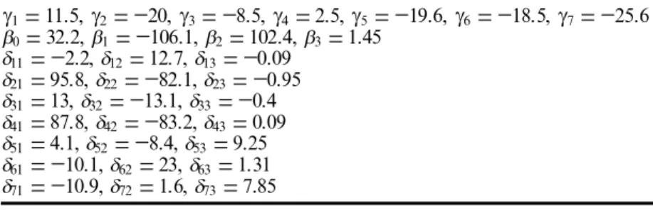
Table 2 lists each of the parameter values.
The SSE for the full model is 699 230 and for the reduced model it is 1 097 690, and the F ratio is then computed as:
F
=
[
SSE(
RM)
SSE(
FM)]
/(
K+1)(
P
1)
SSE(
FM)
/P(
n
K
1)
=
(
1 097 690699 230
699 230/7(
25)
/
[(
33
+11)
)(
7
1)]
=
3.49.Since
Fa
((
K+1)(
P
1)
,P(
n
K
1))
=
F0.05(
24,147)
=
1.6it is larger than Fa
(
24,147)
. Therefore, the null hypothesis is rejected, implying that those operational stages in group 4 cannot be combined into one macro model. It is then initiated to compute the SSE(
FMi)
for each operational stage in step 5.Operational stage 5 is then deleted from the group because its SSE
(
FMi)
is themaximum. Perform step 2 again and the operation stage 13 is further deleted from the group. Finally, the operational stages 4, 9, 15, 18, 20 can be grouped into the equation
Y
=
7.2
117.1Z1+105.4Z2+1.03Z3for F ratio is equal to 1.69 and less than F0.05
(
16,105)
=
1.80.Step 6 then considers the possibility of grouping operational stages 5, 13 in S and ® nds that they can be grouped to the equation
Y
=
23.4
14.2Z1+19.8Z2+1.02Z3for F ratio equal to 1.43 and less than F0.05
(
4,42)
=
2.61. Finally, after passingresiduals analysis that veri® es equal variances among seven stages, all seven opera-tional stages in group 4 can be statistically grouped into the two following regression equations:
Y
=
7.2
117.1Z1+105.4Z2+1.03Z3Y
=
23.4
14.2Z1+19.8Z2+1.02Z3.The total ¯ owtime through all operational stages in group 4 is the sum of two ¯ owtime estimations. The ® rst one is estimated by summing the value of explanatory variables for stages 4, 9, 15, 18, and 20 into the macro equation
Y
=
7.2
117.1Z1+105.4Z2+1.03Z3and the second one is those for stages 5 and 13 into macro equation Y
=
23.4
14.2Z1+19.8Z2+1.02Z3.The same procedure is performed for the groups 1, 2, 3, and 5. The results are listed as follows:
Group 1: operation stages 1 and 7 can be grouped into the equation
Y
=
13.6
0.05(
X1)
+130.1 log(
X2)
+1.09(
X3)
1/2+0.45 log(
X2) (
X3)
1/2Group 2: operation stages 2, 12 and 14 can be grouped into the equation g 1=11.5,g 2= 20,g 3= 8.5,g 4=2.5,g 5= 19.6,g 6= 18.5,g 7= 25.6 b 0=32.2, b 1= 106.1, b 2=102.4, b 3=1.45 d 11= 2.2, d 12=12.7, d 13= 0.09 d 21=95.8, d 22= 82.1, d 23= 0.95 d 31=13, d 32= 13.1, d 33= 0.4 d 41=87.8, d 42= 83.2, d 43=0.09 d 51=4.1, d 52= 8.4, d 53=9.25 d 61= 10.1, d 62=23, d 63=1.31 d 71= 10.9, d 72=1.6, d 73=7.85
Table 2. The parameter value of group 4.
Y
=
10.7
1.1(
X1)
1/2+3.4 log(
X2)
+1.97(
X3)
Operation stages 6, 11 and 21 can be grouped into the equation Y
=
17.3
1.59(
X1)
1/2+152.1 log(
X2)
+0.51(
X3)
Operation stage 17 becomes
Y
=
99.1
0.8(
X1)
1/2+123.3 log(
X2)
+0.3(
X3)
Group 3: operation stages 3 and 8 can be grouped into the equation Y
=
129.2
24.1 log(
X1)
+0.6(
X2)
1/2+0.7X3Group 5: operation stages 10, 16 and 19 can be grouped into the equation Y
=
99.1
0.8(
X1)
1/2+123.3 log(
X2)
+0.3(
X3)
.In summary, the regression equations for all 21 operational stages can be reduced to 8.
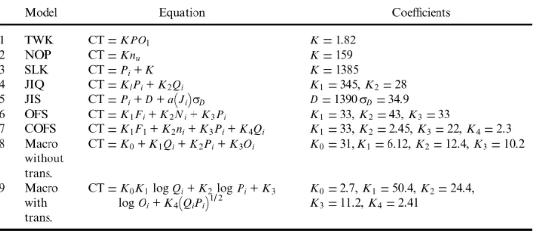
The total estimated ¯ owtime of mixed macro and micro model is then the sum of estimated ¯ owtime of 21 operational stages by summing the value of explanatory variables into 8 macro models instead of 21 micro models. Next, the performance evaluation for our mixed macro and micro model is compared with various macro and micro models (with and without variable transformations) . The reasons why both macro and micro models with and without variable transformation are included in the performance evaluation is to verify whether or not variable trans-formation increases the prediction accuracy at the cost of the di culty to compre-hend. The macro models include seven conventional ¯ owtime estimation models, as proposed by Cheng and Gupta (1989), and two new macro models with and without variable transformations. All de® nitions of explanatory variables for seven conven-tional macro models are the same as those of previous studies except WIP. Apparently, WIP in lots is used to replace the number of jobs in the system. Both new macro models use the same input variables with mixed model except the one without transformation, which uses the original input variables. Table 3 presents the equations and coe cients of the seven models and two new macro ¯ owtime estima-tion models in which the coe cients are acquired by summing the value of expla-natory variables of 21 stages into the macro equation. Table 1 and 4 present the parameters of micro ¯ owtime estimation with and without variable transformation, respectively. The evaluation criteria are based on the factors related to due date performance, e.g. mean absolute deviation, mean square error, mean absolute per-cent error, number of tardy jobs, perper-cent of tardy jobs, average lateness and stan-dard deviation of lateness. Detailed performance measures are taken from Vig and Dooly (1993). Table 5 lists the performance equations and compares the results. The coe cients of regression equations are determined from data from March to August. Meanwhile, seven performance results are generated on the basis of data from September to December where the total observations are n
(
=
8)
. Four important ® ndings are observed.(a) The selection of explanatory variables is critical to the performance of macro models. The relative priorities of the explanatory variables are as follows: ¯ owtime distribution (OFS, COFS, JIS), WIP (JIQ, COFS), processing time (TWK, SLK), and the number of operations (NOP). Selecting the proper combination of explanatory variables can increase the prediction accuracy.
(b) The micro models outperform macro models even if interaction e ects among stages are neglected in this case.
(c) The models with variable transformations outperform those without variable transformations, regardless of whether they are in macro or micro models.
No. Stage name Regression coe cients
1 BPSG2 CVD b 0=3.2, b 1= 1.2, b 2=5.6, b 3= 11.3 2 BPSG2 FLOW b 0=1.4, b 1= 3.2, b 2=4.4, b 3= 3.41 3 3C PHOTO b 0=0.5, b 1= 12.2, b 2=21.1, b 3= 0.19 4 3C ETCHING b 0=2.1, b 1= 132.2, b 2=0.9, b 3= 42.3 5 RTA b 0=0.4, b 1= 142.2, b 2=3.6, b 3= 7.5 6 TI SPUTTER b 0=90.2, b 1= 13.9, b 2=5.0, b 3= 23.2 7 PLANKET W CVD b 0=12.2, b 1= 321.7, b 2=6.2, b 3= 9.63 8 W ETCH BACK b 0=4.2, b 1= 42.2, b 2=0.77, b 3= 31.2 9 BAKING b 0=23.1, b 1= 101.2, b 2=7.6, b 3=21.3 10 WEB SCRUBBING b 0=42.2, b 1= 11.2, b 2=3.5, b 3=7.3 11 AlSiCu SPUTTER b 0=203.2, b 1= 1.2, b 2=44.1, b 3=52.1 12 METAL PHOTO b 0=12.2, b 1= 42.2, b 2=9.1, b 3=1.23 13 METAL ETCHING b 0=93.0, b 1= 31.1, b 2=32.1 b 3=62.7 14 SINTERING b 0=42.2, b 1= 25.2, b 2=1.14 b 3=122.0 15 PAD PSG CVD b 0=52.6, b 1= 47.2, b 2=15.2 b 3=8.9 16 PE-NITRIDE CVD b 0=24.1, b 1= 34, b 2=3.4, b 2=7.4 17 PV PHOTO b 0=52.7, b 1= 541.7, b 2=4.31, b 3=19.3 18 PV ETCH b 0=23.2, b 1= 182.3, b 2=2.77, b 3=6.6 19 PI PHOTO b 0=96.2, b 1= 121.6, b 2=5.1, b 3=7.23 20 UV03 ASHING b 0=104.4, b 1= 51.1, b 2=0.76, b 3=11.7 21 PI CURE b 0=9.2, b 1= 47.1, b 2=3.0, b 3=33.3 Table 4. The parameter value of micro regression without variable transformations. Model 1:ª
Y1=b 10+ b 11X11+ + b 13X13+ e 1 (operation 1).
ª
Y2=b 20+ b 21X21+ + b 23+ e 2
(operation stage 2) . . .Yª 21=b 21,0+ b 21,1X21,1+ + b 21,3+ e 21(operation stage 21).
Model Equation Coe cients
1 TWK CT=KPO1 K=1.82 2 NOP CT=Knu K=159 3 SLK CT=Pi+K K=1385 4 JIQ CT=KlPi+K2Qi K1=345,K2=28 5 JIS CT=Pi+D+a(Ji)s D D=1390s D=34.9 6 OFS CT=K1Fi+K2Ni+K3Pi K1=33,K2=43,K3=33 7 COFS CT=K1F1+K2ni+K3Pi+K4Qi K1=33,K2=2.45,K3=22,K4=2.3 8 Macro CT=K0+K1Qi+K2Pi+K3Oi K0=31,K1=6.12,K2=12.4,K3=10.2 without trans.
9 Macro CT=K0K1logQi+K2logPi+K3 K0=2.7,K1=50.4,K2=24.4,
with logOi+K4(QiPi)1/2 K3=11.2,K4=2.41
trans.
CT=cycle time estimation, Pi=total processing time of product i, ni=number of operations of product i, Qi=WIP in lots of product i, D=Mean waiting in the system,s D=standard deviation of waiting time in the system, Ji=WIP in the system when job I arrives, J=mean WIP in the system,s j= standard deviation of WIP in the system, a(Ji)= 1 if Ji< J s j,=0 if J s j< Ji< J+ s j,=1 if
Ji> J+ s j, Fi=T ni, T=average ¯ owtime per operation for newly completed batches, Oi=move out quantity of product i.
Table 3. Macro models and the model equations.
(d) The performance of the mixed ¯ owtime estimation model ranks between the micro and macro models. In this example, the model complexity reduced by 62% (from 21 equations to 8). Although the prediction error only increases 4% comparing with micro models, two models do not signi® cantly di er. This ® nding con® rms that our mixed model not only reduces the estimation complexity, but also does not degrade the prediction variability.
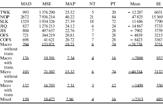
3.2. Example 2
The test procedures for Example 2 are the same as in Example 1 except that the test data are collected from the ® rst 21 stages (instead of the ® nal 21 stages of Example 1) of the 4MB DRAM fabrication process. Table 6 presents the compara-tive performance results.
4. Conclusion
The fact that interaction e ects occur among operational stages accounts for why most investigations on ¯ owtime estimation concentrate on the macro approach instead of the micro approach. From a practical perspective, macro approach models usually do not ® t in long operational stages manufacturing environments, especially in wafer fabrication. Although the micro model reduces the forecast error, the complexity of the estimation model is too high. This study presents a novel mixed macro and micro ¯ owtime estimation model, capable of overcoming the complexity (micro approach) and variability (macro approach) of ¯ owtime estimation, particu-larly for environments such as wafer fab in which hundreds of operational stages are
MAD MSE MAP NT PT Mean SE
TWK 962 1 163 900 23.76 5 20
-
467.88 5394 NOP 2051 6 024 619 36.14 21 84 1821.96 12 273 SLK 1137 1 721 310 25.51 18 72 445.36 6560 JIQ 881 1 161 106 22.17 3 12-
628.88 5388 JIS 598 512 055 14.87 7 28-
300.84 3578 OFS 405 304 129 10.15 9 36-
151.92 2757 COFS 474 382 917 11.13 9 36-
298.2 3094 Macro 271 100 217 17.13 5 20 210.16 2931 without trans. Macro 150 37 464 6.63 4 16 60.99 894 with trans. Micro 200 69 846 12.05 4 16 190.23 1929 without trans Micro 88 12 757 1.94 3 12 41.91 4.19 with trans Mixed 91 13 435 1.99 3 12 45.16 580MAD =mean absolute deviation = njY Yª j/n; MSE =mean square error= n(Y Yª )2/ n;
MAP = mean absolute percentage error = n
jYYª j/ nY ; NT = no. of tardy jobs
=f iji=1, 2,. . ., n and Y >Yª g ; PT =percentage of tardy jobs=(1/ n)f iji=1, 2,. . ., n and Y >Yª g ;
Mean = average lateness =(1/n) n(Y ª
Y); SD = standard deviation of lateness
=(1/ n) n[(Y ª
Y) (1/n) n(Y ª
Y)]2.
Table 5. Performance evaluation for Example 1.
common. According to the result, the proposed model outperforms other conven-tional ¯ owtime estimation models and does not signi® cantly di er from the micro approach. This ® nding con® rms that the mixed model proposed here not only reduces the estimation complexity, but also does not degrade the prediction varia-bility.
The proposed model is developed while assuming that only interaction e ects among explanatory variables of the same stage are considered and those of di erent stages are neglected, Although the assumption is veri® ed in this case, a future inves-tigation should develop a more general model. In addition, variable transformation through stepwise regression obviously increases prediction accuracy at the cost of di culty in comprehension. However, it is unnecessary for the mixed model.
In this study, cycle times are the only input variables. However, more data can be obtained and new factors that can in¯ uence production performance can be included. By doing so, more promising and meaningful models can be developed. Based on the mixed model construction procedure presented in this study, Mosel Vitelic Inc. is planning to construct and implement the performance prediction system.
Acknowledgments
The authors would like to thank the production control department of Mosel Vitelic Inc. for technically supporting this research.
References
Baker, K. R., 1984, Sequencing rules and due-date assignments in a job shop. Management
Science,30, 1093± 1104.
MAD MSE MAP NT PT Mean SE
TWK 993 1 376 290 25.32 5 20
-
12 287 6031 NOP 2672 7 936 214 40.22 21 84 47 825 15 369 SLK 1329 1 934 326 27.39 18 72 11 686 7790 JIQ 827 1 276 213 24.12 6 24-
14 867 5733 JIS 804 497 637 22.76 7 28-
7902 3759 OFS 721 344 219 20.81 7 28-
4839 3215 COFS 698 41 621 20.72 7 28-
8423 3367 Macro 294 133 921 19.71 6 24 28 738 3251 without trans. Macro 176 19 391 7.34 4 16 2800 932 with trans. Micro 193 71 392 15.32 6 24 40 334 2137 without trans Micro 132 16 793 2.31 3 12 1499 530 with trans Mixed 159 18 472 2.96 4 16 2313 695Table 6. Performance evaluation for Example 2.
Baudin, M., Mehrotra, V., Tullis, B., Yeaman, D. and Hughes, R. A., 1992, From spreadsheets to simulations: a comparison of analysis methods for IC manufacturing performance. IEEE/SEMI International Semiconductor Manufacturing Science
Symposium, pp. 94± 99.
Bertrand, J. W. M., 1983, The e ect of workload dependent due-date on job shop perform-ance. Management Science,29, 799± 816.
Bookbinder, J. H. and Noor, A. I., 1985, Setting job-shop due-dates with service-level constraints. Journal of Operation Research Society,36, 1017± 1026.
Chatterjee, S.andPrice, B., 1991, Regression Analysis by Example, 2nd edn (New York: Wiley-Interscience), pp. 107± 110, 227± 251.
Cheng, T. C. E.andGupta, M. C., 1989, Survey of scheduling research involving due date determination decisions. European Journal of Operational Research,38, 156± 166.
Connors, P., Feigin, G. E.and Yao, D. D., 1996, A queueing network model for semicon-ductor manufacturing. IEEE Transactions on Semiconsemicon-ductor Manufacturing,9, 412± 427.
Conway, R. W., Maxwell, W. L. andMiller, L. W., 1967, Theory of Scheduling (MA: Addison-Wesley).
Eilon, S. and Chowdhury, I. G., 1976, Due-date in job shop Scheduling. International
Journal of Production Research,14, 223± 238.
Enns, S. T., 1995, A dynamic forecasting model for job shop ¯ ow time prediction and tardi-ness control. International Journal of Production Research, 33, 1295± 1312.
Heard, E. L., 1976, Due-dates and instantaneous load in the one-machine shop. Management
Science, 23, 444± 449.
Karmarkar, U. S., 1987, Lot sizes, lead time and in-process inventories. Management
Science, 33, 409± 418.
Lawrence, S. R., 1995, Estimating ¯ owtimes and setting due-dates in complex production systems. IIE Transactions,27, 657± 668.
Lynes, K.and Miltenburg, J., 1994, The application of an open queueing network to the analysis of cycle time, variability, throughput, inventory and cost in the batch produc-tion system of a microelectronics manufacturer. Internaproduc-tional Journal of Producproduc-tion
Economics, 37, 189± 203.
Philipoon, P. R. and Fry, T. D., 1992, Capacity-based order review/release strategies to improve manufacturing performance. International Journal of Production Research,30, 2559± 2572.
Ragatz, G. L. and Mabert, V. A., 1984, A simulation analysis of due-date assignment rules. Journal of Operations Management,5, 27± 39.
Seidmann, A. and Smith, M. L., 1981, Due date assignment for production system.
Management Science,27, 571± 581.
Srivatsan, N.and Kempf, K., 1995, E ective modeling of factory throughput times. IEEE/
CPMT International Electronics Manufacturing Technology Symposium, pp. 377± 383.
Udo, G. J., 1992, Neural networks applications in manufacturing processes. Computers and
Industrial Engineering, 23, 97± 100.
Vig, M. M. 1989, Dynamic estimation of job ¯ ow time. Masters thesis, University of Minnesota, Twin Cities, USA.
Vig, M. M. andDooly, K. J., 1991, Dynamic rules for due-date assignment. International
Journal of Production Research, 29, 1361± 1377. 1993, Mixing static and dynamic ¯ ow
time estimates for due-date assignment. Journal of Operations Management, 11, 67± 79.
Weeks, J. K.and Fryer, J. S., 1977, A methodology for assigning minimum cost due-dates.
Management Science,23, 872± 881.
Weeks, J. K., 1979, A simulation study of predictable due-dates. Management Science, 25,
363± 373.
Wein, L. M., 1991, Due-date setting and priority sequencing in a multiclass M/G/1 queue.
Management Science,37, 834± 850.
Zhang, H. C.and Huang, S. H., 1995, Applications of neural networks in manufacturing: a state-of-the-art survey. International Journal of Production Research, 33, 705± 728.