OPTIMIZATION OF 2-DIMENSIONAL RADOME BORESIGHT ERROR PERFORMANCE USING SIMULATED ANNEALING TECHNIQUE

Optimization of Two-Dimensional Radome

Boresight Error Performance Using

Simulated Annealing Technique

Fang Hsu, Po-Rong Chang, Member, IEEE, and Kuan-Kin Chan, Member, IEEE

Abstract-In this paper a systematic approach to radome design is presented. The problem is formulated as a global optimization procedure such that the radome performance is optimized by properly adjusting the thickness of the radome layer over the entire radome surface. In this approach the thickness profile is parameterized via B-splines representation. Simulated annealing technique is applied to finding the best thickness profile so that the maximum boresight error is re- duced as small as possible over the entire range of the antenna look angle. A two-dimensional design example is given. The best possible thickness profile is found and the boresight error is reduced considerably compared to that due to a uniform layer. The method is general and can be applied without difficulty to other realistic three-dimensional radomes of arbitrary shapes.

I. INTRODUCTION

S a dielectric layer, the radome inevitably introduces

A

pointing error with respect to the apparent look angle of the radar antennas. In the past, major re- searchers have concentrated on the analysis of the bore- sight error (BSE), which is a major consideration in radome performance. Since in practice the shapes of radomes often conform to aerodynamic requirements of the radar housing, such as the missiles, the aircraft, etc., no rigorous electrical analysis is possible except for a few simple geometries. One must therefore resort to some approximation methods. Early investigators employed the geometrical optics and surface integration [ 11 technique. The fields on the outer surface of the layer are first obtained via ray-tracing, and the equivalence principle is employed next to evaluate the radiation fields. By the plane-wave spectrum technique [2], the ray-tracing is re-

placed by constituents of plane waves and therefore the transmitted fields can be found by simply approximating the local radome layer as slab, and thus the solution corresponding to the slab problem can be applied. Further improvement [3] makes use of the cylindrical wave spec- trum and approximates the local layer as circular in order to take into account the curvature effect.

One notes that all the literature relates to the perfor- mance evaluation of the radome; little has been published

Manuscript received May 5, 1993. This work was supported by the National Science Council of R.O.C. under Contract CS80-0210-DOO

The authors are with the Department of Communication Engineering, IEEE Log Number 9212511.

9-26.

National Chiao Tung University, Hsinchu, Taiwan, Republic of China.

concerning the design issue, i.e., to improve the perfor- mance such as to minimize the boresight errors. In this paper, we develop a systematic method to address this problem. As a specific example, we require that for a

specified shape of the radome, the boresight error is minimized over the entire range of the antenna look angle through proper adjustment of layer thickness over the radome. The problem is formulated as a global optimiza- tion procedure in which the radome performance as cost function is to be optimized. Constrained optimization is also considered by way of examples. In Section I1 we start by problem specification and formulation. Section I11 gives the surface modeling. Global optimization is introduced in Section IV. In Section V we apply our technique to a

design example, and the numerical result is presented in Section VI. The conclusions are in the last section.

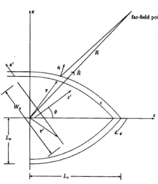
11. PROBLEM SPECIFICATION AND FORMULATION Fig. 1 depicts a two-dimensional (2D) antenna-radome system. The radome layer is made of dielectric material with permittivity E , which is assumed to be constant as in

practical situations. The antenna is represented by a y - directed constant-density current sheet of infinite extent over the width W,. A time dependence e l m f is assumed and omitted throughout. The outer radome surface s is assumed to be specified. As a design objective, we look for the inner surface, and hence the thickness profile d ( s ) along the surface, such that the boresight error over the entire antenna look angle is made as small as possible. For simplicity, the rate of change of the boresight error is not considered in this paper, though it can be incorpo- rated into the optimization algorithm.

A. Fields on the Outer Surface of the Radome

To find the field at any point on the outer surface, we adopt a slightly different approach than that found tradi- tionally. We approximate the local surface as a slab of infinite extent; therefore, the fields on the outer surface can be found in terms of the dyadic Green’s function, denoted as G , corresponding to the slab problem, i.e.,

E ( s , d ) =

///

G , ( s , r ’ ) J ( r ‘ ) dr’, H ( s , d ) =

///

G , ( s , r’>J(r’> dr‘, (1) (2) aP aP 0018-926X/93$03.00 0 1993 IEEE

1196 IEEE TRANSACTIONS ON ANTENNAS AND PROPAGATION, VOL. 41, NO. 9, SEPTEMBER 1993 B. Radiation Fields in the Presence of the Radome

By the equivalence principle [6], the fields transmitted through the radome can be evaluated by making use of the equivalent current distribution over the outer surface. The equivalent electric and magnetic surface currents are given respectively as J, = fi X H and M, = E X fi. The resulting potentials are

1 J,( r’)e -jkoir- r’ 1 A =

-//

Ir - r’l da’ ,

45-

and therefore in free space the electric field can be found through

1

J W E

E = - V X F + - V X V X A . (8)

For a 2D problem shown in Fig. 1, the electric field has only a y component E , which can be simplified as E = -/H,$2)(koR)Ht k,2 ds

4WEO s

Fig. 1. Geometry of a two-dimensional antenna-radome system.

- jkO T / H 1 2 ) ( k , , R ) ( f i * k ) E , ds, ( 9 ) where s defines a parametric representation of the outer

surface and d = d ( s ) is the thickness at s. G, and G , are respectively the Green’s functions for the electric and magnetic fields corresponding to the slab problem. Notice that the Green’s functions are functions of parameter s of the curve length in the 2D case. For specified 2D radome profile, the last W O integrals become W O line integrals

over the antenna width, and the Green’s functions as

S

Where H1 and E, are tangential field components on the m h m e surface p d fi is the o u t ~ a r d unit vector on the surface. R is the unit vector from the outer surface of the radome to the observation point. HA2’ and Hf2’ are respectively the Hankel functions of the second kind of order 0 and 1.

functions of d ( s ) have the spectral representations [41

_c.

_{Boresight and Global}

where k , is the wave number, p is the distance, and

4

is the incident angle from the source point to the radome’s inner surface. E , is the free space permittivity. T ( w , d(s))

is the plane-wave transmission coefficient [51 for the pla- nar slab of thickness d(s), which is given as

where

K = k , COS w , K€ = k,-,

The boresight error S is defined as the angular devia- tion of the antenna beam maximum in the presence of the radome from that without the presence of the radome. Previous discussion states that for a specified antenna look angle 8, S varies as a functional of the thickness profile d(s). On the other hand, for specified d(s), S varies as a function of 8. Therefore

6 = S ( 8 , d ( s ) ) . (10)

The optmal radome design, as we defined it in this partic- ular application, is to find the optimum S throughout the whole range of d ( s ) and 8. By optimization, we adopt the minimax criterion, i.e.,

(11)

min max S ( 8 , d ( s ) ) ,

d ( s ) @

with the maximum operating on the whole range of 8 and the minimum on d(s), which is nonnegative. However, a trivial case should be excluded for which d ( s ) = 0. More- over, in practice, d ( s ) should not deviate dramatically from a nominal value do. In summary, the optimal radome design problem is formulated as to

subject to a nominal specification

maxId(s) - d o l I E , (13)

where E might be taken, for example, as a proper fraction

of do. Consequently, (12) becomes a constrained minimax optimization problem.

111. CUBIC B-SPLINE REPRESENTATION OF THE THICKNESS PROFILE FUNCTION

In general, the process of optimal design requires a finite number of unknown parameters to be determined, whereas in (121, d(s), which is a continuous function of s, imposes infinitely many possible unknown parameters as- sociated with its amplitude corresponding to each location at s. Clearly, it is hard to find an optimal thickness profile by the ordinary finite-parameter optimization techniques. To circumvent this difficulty, a transformation of the parametric representation of the thickness profile be- comes necessary. This can be done, for example, by simple Fourier representation. However, here, a natural candi- date for the thickness profile d ( ~ ) is suggested to be the well-known cubic B-spline representation, which can be expressed as

N + 1

d ( s ) = P j B j W , (14)

where Bj's are the spline basis functions and

pi's

are the expansion coefficients to be determined. Even though (14) is an approximation, it can be made as accurate as desired for sufficient large N . Then the problem of (12) can be parameterized as

i = -1

subject to the same nominal specification constraint as mentioned in (13). Equation (15) is regarded as a standard form in the theory of global optimization.

A. Spline Space and B-splines

Before giving a formulation of the B-spline representa- tion, we introduce some definitions [71.

Definition: Given the interval [a, b ] of the real line, let

6

denote the discrete set of N

+

1 points and a =

to

<

t1

<

-..

<

tN

= b. The spline space S , ( t ) of degree

m is defined by S , ( t ) = { g ( O E C m - ' [ a , bl; g ( t ) is a

polynomial of degree m on each interval [

t,, tl+l],

i = 0, l,..., N - l}. For a given spline space S m ( t O , . . . ,

t,,,),

it always associates with further points C-,

<

<

t-l

<

a and b

<

tN+'

<

<

tN+,,

where these points may be chosen arbitrarily.

Lemma: For each i E { -m,..., N - 1}, there exists a unique spline B,", called B-spline, of degree m with knots

t-,,...,

t N + ,

such that

B y ( t ) = 0 t ~ ( - 0 0 ,

(,I

U [ t l + , + l , O O ) , (16)

B,"

>

0 t E

(ti,

t i + m + I ) , (17)

(18)

Accordingly, a spline is a piecewise polynomial function with derivative continuity condition at each fixed knot. It is shown [8] that any continuous function, say f , can be approximated to arbitrarily high accuracy by a spline of degree m , provided that the spacing between knots is sufficiently small. In the case of m = 3 and the uniform

spacing between points

ti+

and

t j ,

i = 0, l,..., N - 1 (i.e., h = for all i), it had been proven that

there exists a spline s E S, which has the approximation error of order 4, that is,

-

(19)

B-splines are specific splines which satisfy a few more constraints and form a basis of any spline spaces [7]. B-splines are splines which have the smallest possible support. Moreover, a stable evaluation of B-splines with the aid of a recurrence relation is possible. Thus B-splines are a popular choice of piecewise polynomial interpola- tion. Cubic polynomials are the most frequently used for splines since they are the lowest order in which the curvature can change sign and have the minimum mean squared curvature. Based on the above facts, the cubic B-splines are chosen to model the thickness profile func- tion (TPF).

B. TPF Interpolation by Cubic B-splines

In the two-dimensional case, the TPF can be expressed by a curve 4 s ) with abscissa of curve length s. Moreover, without loss of generality, the curve length s can be normalized to unity such that the TPF curve can be represented by d( p) with the range that p E [O, 11. As-

sume that ( N

+

1) points located on the TPF curve are chosen and denoted by ( p j , d( pi)), where p i = i / N and

i = 0, l,..., N . Those points are also called the knots of

the associated interpolation spline. [9] shows that the resulting cubic spline representation of the TPF curve can be generated by these chosen N

+

1 knots and described bY

Nf 1

d ( p ) = PiB(i - N p ) , (20)

j = - 1

where

pi

is the ith unknown expansion coefficient and

B(i - N p ) (i.e., B?) is its associated cubic spline basis

function. The cubic spline function has a characteristic bell shape and can be described by the following five equations: B ( 7 ) = ( 2

+

d 3 / 6 - 2 1 7 1 -1, = (4 - 67' - 3 ~ ~ ) / 6 - 1 I 7 I 0, = (4 - 67'

+

3 ~ ~ ) / 6 0 I 7 I 1, = (2 - d 3 / 6 1 5 7 5 2 ,

= o

2 I 171, (21)

1198 IEEE TRANSACTIONS ON ANTENNAS AND PROPAGATION, VOL. 41, NO. 9, SEPTEMBER 1993 where T = Np. The N

+

1 chosen knots are substituted

into (20) to yield

1

Observing (22), there are ( N

+

3) unknown variables

pi

involved in ( N

+

1) linear equations that cannot give an unique solution. In order to tackle this difficulty, we need two more independent linear equations. These two equa- tions can be obtained by placing the clamped end con- straints [9] on the both ends of the curve, which in this

case will be to fix the gradient at the ends. The clamped end condition is used to determine the shape at the ends of a spline. The gradients at the ends will be denoted by go and gN. To compute them, the interpolation spline

equation has to be differentiated with respect to p, giving

d ' ( p ) = N &B'(Np - i). (23) N + 1

i = -1

and

(25)

Usually, the gradient at the ends is specified by the user, or alternatively can be set to some default value. Combin- ing (221, (241, and (251, it can be summarized in a compact

matrix form where M a p = d , (26) -N/2 0 N/2 0 1/6 2/3 1/6 0 0 1/6 2/3 1/6

I

0 0 0

I

a

0

o

0

o

o

0

It can be easily shown that det ( M I # 0; such an expan- sion coefficient vector

p

can be calculated by direct matrix inversion:

p

= M-' . d . (30)

Equation (30) shows that there is a one-to-one mapphg

between and d implicitly. Once d is chosen,

p

is determined uniquely. Consequently, the cost function m a o

N e ,

p-l,--., pN+l)

of (15) is then in terms of d =

' (d( pol, d( pl),*--, d( pN)). Therefore, the constrained minimax optimization problem can be solved with respect to a set of new variables d( p O ) ; - * , d( pN). This yields I min max

H e ,

d( po),..., d( p N ) ) . (31)

IV. OPTIMIZATION BY SIMULATED ANNEALING TECHNIQUE

Simulated annealing is a recently developed and cost- effective approach to solving the combinatorial optimiza- tion problems. Kirkpatrick et al. [lo] first recognized a

strong analogy between physical annealing and solving large combinatorial optimization problems. In simulated annealing, the possible solutions of a combinatorial opti- mization problem are analogous to the states of a physical system, the cost of a given solution is analogous to the energy of a given state, and the control parameter T, is analogous to the temperature of a heat bath.

An instance of a combinatorial optimization problem

[ l l ] can be formalized as a pair

W,f)

where the solution state space U denotes the finite set of possible solutions and the cost$nctionf is a mapping defined as f : U + 'ill.

Hence, the goal of combinatorial minimization is to fmd the solution uOpt E U such that f(uopt) ~ f ( u , ) for all

u i E U. This goal may be achieved by using the following

proposed simulated annealing algorithm.

Simulated annealing is a smart random search tech- nique which is often more efficient than exhaustive search yet more robust than gradient descent. The search process of the simulated annealing is controlled by an externally specified parameter, usually called effective temperature, T,, with the same units as the cost function. When T, is relatively large compared with the maximum value of the cost function, simulated annealing explores the entire solution space using a uniformly generated random per- turbation which is a transition from the current state (state ui with cost f ( u i ) ) to the proposed state (state u j

d ( p o ) ; . . , d ( l L N ) 0 0 0 *.. 0 0 0 0 0 ..* 0 0 0 0 0 * * * 0 0 0

.

.

...

.

,

...

0 0 *.. 1/6 2/3 0 0 0 *.* 1/6 2/3 1/6 0 0

..*

-N/2 0 N/2 (29)

with cost f ( u j ) ) , and with no preference for lower cost function. As T, gets smaller, this undirected eploration

changes. When T, is small enough, simulated annealing becomes a descent algorithm. At intermediate values of T,, the simulated annealing moderates its behavior be- tween these two extremes: The transition is immediately accepted if f ( u j ) is less than or equal to f(u,); otherwise, it is accepted with a probability given by the Boltzmann distribution e(f(ui)-f(uj))' 'e. By gradually decreasing T,, the

M := 0

4

Yes

uj:="state generated by state transition procedure"

Fig. 2. Flow diagram of simulated annealing technique.

search is systematically concentrated into regions likely to contain a global minimum, but still random enough to escape most local minimum. Ref. [ l l ] shows that the convergence to the global minimum is provable with prob- ability 1 sense.

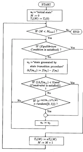
The algorithm can be best understood in the flow diagram shown in Fig. 2; it is observed that there are two nested loops involved in the simulated annealing algo- rithm. The outer one will be terminated when the number of iterations, M , is equal to a sufficiently large value M,,, , which could be obtained by a priori measure for the lowest effective temperature. And the inner loop stops if the equilibrium condition [121 is satisfied. In addition, a cooling process [ l l l should also be used to control the decrement of T,, and is given by T,(M

+

1) = a T , ( M ) , where M is the index of the iteration for the outer loop, and the control parameter reduction factor, a, is between

0.95 and 1. The initial effective temperature T,(O) should be chosen so that the initial transition-acceptance ratio is high [ll].

It should be mentioned that the condition of reaching an equilibrium point at the nth iteration can be deter- mined by the following equations:

n

where

t

is a specified criterion and AVEaccept is the estimate of the average of the accepted cost functions and given by

(33)

where naCcept is the number of acceptions.

V. RADOME DESIGN BY SIMULATED ANNEALING In this section, the simulated annealing approach will be incorporated into the problem of radome design. To solve the optimization problem (31), a solution state is chosen as the ( N

+

1)-dimensional vector

= (d( pO),*", d( P N ) ) , (34) where d( p i ) is the value of thickness at knot i . The value of the cost function is taken as the maximal boresight error, which can be estimated by choosing the maximal value of the boresight errors which correspond to a num- ber of sampling angles within the antenna's scan range. Suppose that there are p sampling angles belonging to the scan range, that is,

e,,

j = l , . . * , p ; then the estimated maximal boresight error becomes

Clearly the estimate can be made as accurate as desired for sufficiently large p . Since the radome thickness cannot be too thick or too thin in practical sense, it is required that the thicknesses d( p i ) ( i = O,..., N ) satisfy the follow- ing boundness constraint:

d m j n 2 d( P , ) 5 dmax 7 (36)

where d,, and d,,, denote the lower and upper bounds of d ( p , ) , respectively. As discussed in Section IV, a combinatorial optimization problem can be executed suc-

cessfully by using the simulated annealing technique when the solution state space is finite. Unfortunately, the possi- ble number of states belonging to the feasible range of d( p , ) is infinite. This truly contradicts the requirement of the finite state space. To overcome this difficulty, a realis- tic way is to use a sampling method. By the method of sampling the closed interval [dmin, d,,,], the possible val- ues of the thickness of d( p,) will form a finite set, i.e.,

(37) d( pi) E (b,lk = l , . . . , 4 ) E b , ,

where

1200 IEEE TRANSACTIONS ON ANTENNAS AND PROPAGATION, VOL. 41, NO. 9, SEPTEMBER 1993

(F)

randomly in (0,. . . , N } " r f := max(r1, rz) r - := min(r1, r2)

9

IF ( k 5 N ) ?

1

Yes

I

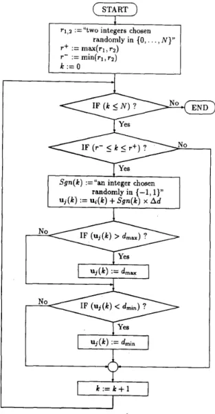
Fig. 3. Flow diagram of the state transition procedure. Ad is the sampling interval.

Consequently, the finite discrete solution state space of the constrained minimax optimization problem can be expressed as the N Cartesian's product of ( N

+

1) sets

and given by

(39)

with the size of the space (total number of states) IUI given as

IUI = ( N

+

l)! (40)

Therefore, the process of finding a minimax boresight error solution becomes a combinatorial optimization problem characterized by a pair (U, i3max(u)), where U and Sm&) are the finite solution space and the cost function, respectively. Undoubtedly, the simulated annealing algo-

U

= b , X b , X *.* x b ,

,

.

-,

N + 1 terms

rithm can be utilized to find the global minimax solution over the feasible space directly. Meanwhile, a smart state transition procedure procedure based on the previous state and its local perturbation is conducted to improve the effectiveness of the original simulated annealing tech- nique. The procedure is described via the flow diagram as shown in Fig. 3.

. VI. DESIGN EXAMPLES

For illustration purpose the method has been applied to the design of a two-dimensional ogival radome as depicted in Fig. 1. Here the dielectric constant of the radome is

assumed to be 4. A loss tangent ranging from 0 to 0.002 is

incorporated into the design examples. The frequency of operation is 10 GHz. L, = 6A and

L,

= 12h where h is the free-space wavelength. The maximum scan angle of the antenna is 45" about the ogive axis.

Our numerical program is carefully checked for each

module in the design. For special case E = 1, which corre- sponds to the removal of the radome, there exhibits an inherent numerical error about 0.01' , marked as curve E in each of the following figures. This in effect establishes a criterion with which the performances of the optimized design can be compared. In the surface integration to acquire the far fields, the integration is extended to 90" with respect to the main beam in order to achieve suffi- cient accuracy.

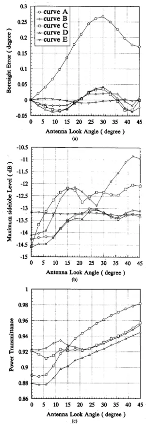
Fig. 4 shows the resulting designs for various design objectives, where curve A refers to the initial layer of uniform thickness which is to be optimized. The material

has a dielectric constant E = 4 - j0.002. The BSE reaches

the peak level of 0.27' at the antenna look direction of 30". After optimization, the resulting BSE curve B is reduced considerably to 0.02" maximum, a dramatic im-

provement compared with the inherent error of 0.01'. However, as shown in Fig. 4(b), the maximum sidelobe level deteriorates as a result of the optimization with the BSE as the sole optimization goal. To overcome this, a multiobjective optimization is possible, with both BSE and sidelobe level incorporated into the objective function. But for simplicity we can equally impose a constraint on the sidelobe level in our optimization algorithm, as can be seen in the flow diagram in Fig. 2. Curve C corresponds to

BSE optimization with the constraint that the maximum sidelobe level is restricted to -12 dB, while curve D corresponds to the constraint of sidelobe level of

-

13 dB,

which approximately equals that due to the uniform layer. Compare D with C; the BSE is only slightly degraded. Notice that from Fig. 4(a) the boresight error rate is not adversely affected after optimization in most cases, except perhaps in the large scan angle. This, as well as other performance measures, can be improved if necessary by simply imposing them as constraints in the optimization loop. We also plot the power transmittance versus the scan angle in all cases; except for the trivial case E = 1 for

which the total transmittance is 1. It appears that at low scan angle before reaching 15', curves B and C have more power transmitted than that of the uniform layer. The

0.3 0.25 h

8

0.2

9

8

5

'0 0.15 0.1

'g

0.05 0 -n.w 0 5 10 15 20 25 30 35 40 45 Antenna Look Angle ( degree )

(a)

Q

-115 W m

1

-12

+

H -12s -13 -135

f

-14

E

-14.5 l " . .. . . . . 1 0.98

3

0.96 .%

cl

0.92 1

!!

o.94

1

0.9 .I . . . , .,.. . ... 0.88 0.86 0 5 10 15 20 25 30 35 40 45 Antenna Look Angle ( degree )

(C)

Fig. 4. Radome performance parameters for: case A radome charac- teristics for uniform layer before optimization; case B: optimized charac- teristics without constraint; case C optimized characteristics with side- lobe constraint - 12 dB; case D: optimized characteristics with sidelobe constraint - 13 dB; case E: trivial case E = 1; inherent numerical error is shown for boresight error.

20 25 30 35 40 45 50 55 60

Observation Angle ( degree )

Fig. 5. Relative power patterns with antenna at look angle 0 = 42"

e = 4 - j0.002. 0.82

g

0.8

b

0.78

a

0.76 0.74 0.72 0.7

4

8

0 0.1 0.2 0.3 0.4 0.5 0.6 Curve length : m

Fig. 6. Optimized thickness profle functions for cases B, C, and D.

situation reverses for scan angle passing beyond 15". The field patterns corresponding respectively to the curves A, B, and D are plotted in Fig. 5 , with the antenna scanned at 42", in which direction it exhibits the highest sidelobe

level if the constraint is not imposed. The optimized thickness profiles for cases B, C, and D are shown in Fig. 6.

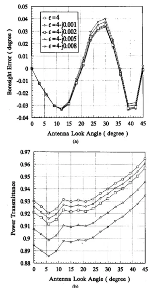
The effect of the dielectric loss on the optimal design is shown in Fig. 7. The boresight error is optimized for

E = 4 -J0.002. Observe that the loss tangent in the typi-

cal range has little effect on the optimized BSE and therefore in this case it will not be necessarily taken into serious consideration in optimal design. The sidelobe level is essentially unchanged for all loss cases.

In the above example the antenna is represented by an electric current sheet. Thus the polarization is perpendic-

1202 IEEE TRANSACTIONS ON ANTENNAS AND PROPAGATION, VOL. 41, NO. 9, SEPTEMBER 1993 0.05

1

I

I

0.04 0.03

8

!3

0.02 a W 8 0.01 t: W O -0.01

E

a

-0.02 -0.03 0 5 10 15 20 25 30 35 40 45 Antenna Look Angle ( degree )

(a) 0.97 L I 0.96 0.95 8

9

0.94 .t:

1

0.93

9

g

0.92 I - t . '" '11 1"~~~ "'~~''" '"'"'' 0 5 10 15 20 25 30 35 40 45 Antenna Look Angle ( degree )

Fig. 7. Effects of the dielectric loss on (a) optimized boresight error

(b)

and (b) power transmittance.

ular to the plane of scan ( H plane) of the antenna. Both polarizations are present in practical three-dimensional configurations. For a comparison of the behavior of the two polarizations on the BSE, we replace the electric current sheet by a magnetic current sheet. The results are shown in Fig. 8. It is observed that the maximum BSE is 0.4" before optimization. The optimal result we obtained is 0.068", which is a considerable improvement over the uniform layer. The boresight error rate is somewhat de- graded near the forward direction and at large scan angle. Optimization design usually costs a large amount of computation time since it involves many times of iterative calculations before reaching the desired performances. In our case, it takes a large amount of calculations to find the field transmitted through the layer as well as to evaluate the radiation fields by surface integration. To save computation, we adopt a curve-fitting technique such

+optimized layer +inherent error 0.35 n 1 -0.1 ' ' ' ' ' ' ' I ' ' ' ' I ' ' ' ' I ' ' ' ' ' ' ' ' ' ' ' '

'

' ' ' ' I ' ' ' '

'

0 5 10 15 20 25 30 35 40 45 Antenna Look Angle ( degree )

Fig. 8. Boresight error due to a magnetic current sheet for uniform layer, optimized layer without constraint, and inherent numerical error for E = 1.

that the transmitted fields through the layer as a function of the layer thickness deviated from its nominal values are first computed and then properly fitted by a polynomial which is stored and retrieved for each iteration. The number of coefficients of the polynomial should be taken sufficiently large in order to ensure the accuracy of the computation.

The optimal result depends also on the number of the control points N, = N

+

1 as well as the number of the sample points q for modeling the thickness profile of the layer. A few trials indicate that the best possible result can be obtained for N, = 11 in our design example. Be- yond that the improvement on BSE is well within the range of the inherent numerical error. For N, = 11 and q = 69, it takes 7702 iterations of search to reach the desired result. The optimization is performed on an IBM 6000/560 workstation at the cost of CPU time 4.193 hours. With constraint it takes about 5000 iterations and 10.5 CPU hours. It should be noted that additional 20 CPU hours are required to set up all the coefficients of the polyno- mial on curve fitting.

VII. CONCLUSION

We develop in this paper a systematic approach to optimal radome design. The problem is formulated as a global optimization procedure such that the radome BSE performance is optimized by properly adjusting the thick- ness of the radome layer over the radome surface. A

two-dimensional example is presented to show the effec- tiveness of our design approach. In principle, the method is general and can be applied to other complicated struc- tures as well, such as the three-dimensional and unsym- metric one. In that case, it needs only to replace the two-dimensional BSE calculation by the three-dimen- sional one, while the radome is modeled by the spline surfaces [9].

ACKNOWLEDGMENT Chung Chen Institute of Technology, Taiwan, Republic of China. His current research interests are in the area of wave propagation in anisotropic media and applications of optimization methods in applied The authors would like to thank the reviewers for their

helpful comments. electro magnetics.

REFERENCES

G. Tricoles, “Application of ray tracing to predicting the proper- ties of a small, axially symmetric, missile radome,” IEEE Trans. Antennas Propagat., vol. AP-14, pp. 244-246, Mar. 1966.

D. C. F. Wu and R. C. Rudduck, “Plane wave spectrum-surface integration technique for radome analysis,” IEEE Trans. Antennas Propagat., vol. AP-22, pp. 497-500, May 1974.

J.-H. Chang and K.-K. Chan, “Analysis of a two-dimensional radome of arbitrarily curves surface,” IEEE Trans. Antennas Prop- agat., vol. AP-38, pp. 1559-1568, Nov. 1990.

L. B. Felsen and N. Marcuvitz, Radiation and Scattering of Waves.

New Jersey: Prentice-Hall, 1973.

R. E. Collin, Field Theory of Guided Waves. New York McGraw- Hill, 1960.

R. F. Harrington, Time-Harmonic Electromagnetic Fields. New York McGraw-Hill, 1961.

Giinther Niimberger, Appa’mation by Spline Functions. New York Springer-Verlag, 1980.

M. J. D. Powell, Approximation Theory and Method. Cambridge, England Cambridge University Press, 1981.

Peter Burger and Duncan Gillies, Interactive Computer Graphics. New York Addison-Wesley, 1989.

S. Kirkpatrick, C. D. Gelatt, and M. P. Vecchi, “Optimization by

simulated annealing,” Science, vol. 220, pp. 671-680, 1983. E. Aarts and J. Korst, Simulated Annealing and Boltzmann Ma- chines: A Stochastic Approach to Combinatorial Optimization and Neural Computing. New York Wiley, 1989.

F. Catthoor, H. de Man, and J. Vandewalle, “SAMURAI: A general and efficient simulated-annealing schedule with fully adap- tive anenaling parametes,” ESZ J., vol. 6, pp. 147-178, 1988.

Fang Hsu was bom in Taiwan, Republic of China, in 1959. He received the B.S. degree from Chung Cheng Institute of Technology and the M.S. degree from National Tsing Hua Uni- versity, in 1981 and 1986, respectively, both in electrical engineering. Currently, he is pursuing the Ph.D. degree in electronics engineering at National Chiao Tung University, Hsinchu, Tai- From 1986 to 1989, he was an Instructor in

the Department of Electrical Engineering, Wan.

Po-Rong Chang (M’87) received the B.S degree

in electrical engineering from National Tsing Hua University, Taiwan, in 1980, the M.S. de- gree in telecommunication engineering from National Chiao Tung University, Hsinchu, Tai- wan, in 1982, and the Ph.D. degree in electrical engineering from Purdue University, West Lafayette, IN, in 1988.

From 1982 to 1984, he was a Lecturer in the

Chinese Air Force Telecommunication and

Electronics School for his two-year military ser- vice. From 1984 to 1985, he was an Instructor in thi Department of Electrical Engineering at National Taiwan Institute of Technology, Taipei, Taiwan. From 1989 to 1990, he was a project leader in charge of SPARC chip design team at ERSO of Industrial Technology and Re- search Institute, Chu Tung, Taiwan. currently he is an Associate Profes- sor in the Department of Communication Engineering at National Chiao Tung University. His current interests include fuzzy neural network, HDTV color signal processing, and human visual and audio system.

area of electromagne :tic

Kuan-Kin Chan (M’88) was bom in China in

1943. He received the B.S. degree in electrical engineering from Cheng Kung University in

1966, the M.S. degree in electronics from Chiao Tung University in 1969, and the Ph.D. degree in electrophysics from Polytechnic Institute of Brooklyn, Farmingdale, NY, in 1976.

Dr. Chan is now a Professor in the Depart- ment of Communication Engineering, National Chiao Tung University, Taiwan, Republic of China. His current research interests are in the