地下水污染源歷程重建-模擬退火演算法

國 立 交 通 大 學

環 境 工 程 研 究 所

碩 士 論 文

地下 水污 染 源歷 程重 建

地下 水污 染 源歷 程重 建

地下 水污 染 源歷 程重 建

地下 水污 染 源歷 程重 建 ：

：

： 模 擬退 火 演算 法

：

模 擬退 火 演算 法

模 擬退 火 演算 法

模 擬退 火 演算 法

Reconstructing the Release History of a Groundwater

Contaminant Using Simulated Annealing

研 究 生：陳 淇 汾

指導教授：葉 弘 德 教授

地下水污染源歷程重建：模擬退火演算法

Reconstructing the release history of a groundwater

contaminant using simulated annealing

研 究 生 ： 陳淇汾

Student：Chi-Fen Chen

指導教授： 葉弘德

Advisor：Hund-Der Yeh

國 立 交 通 大 學

環 境 工 程 研 究 所

碩 士 論 文

A Thesis

Submitted to Institute of Environmental Engineering

College of Engineering

National Chiao Tung University

in Partial Fulfillment of the Requirements

for the Degree of

Master of Science

in

Environmental Engineering

June, 2006

Hsinchu, Taiwan

中 華 民 國 九 十 五 年 七 月

地下水污染源歷程重建：模擬退火演算法

研究生：陳淇汾 指導教授：葉弘德

國立交通大學環境工程研究所

摘 要

摘 要

摘 要

摘 要

當一個場址發現地下水有污染，且其已知污染源位置上曾更替過

數個工廠或工廠的經營者時，重建污染源釋放歷程將可協助

釐清各可

能責任團體之責任歸屬問題。

本研究

利用函數擬合技巧，結合模擬退

火演算法(simulated annealing, SA)與地下水

污

染傳輸控制方程式之基

本解，來推算地下水污染源釋放歷程。其重建步驟為:首先，將已知

釋放地點之真實污染源釋放函數代入地下水

污

染傳輸控制方程式之

基本解中，計算得到監測井的污染物濃度值，然後設定此值為採樣濃

度。其次視該污染源的釋放函數為未知，並假設其由多項指數函數所

組成；利用 SA 試誤產生未知函數中的參數值，得到試誤之污染源釋

放函數。隨後，將試誤函數代入地下水

污

染傳輸控制方程式之基本解

中，計算出監測井的模擬濃度值。根據模擬濃度與採樣濃度之最小誤

差平方和，SA 最後能搜尋到假設函數中之最佳參數值；若將此函數

算出或畫出圖形曲線，則得以重建地下水污染源的釋放歷程。

為了模擬現地可能之情形，本研究分析的案例，從一維點源傳輸

問題擴展至二維與三維非點源傳輸案例；另外考慮含水層為有限寬度

與無限寬度兩種不同狀況。本研究除了調查監測井與污染源的距離對

重建結果的影響，同時也針對幾項問題進行探討，分別是時間性數據

與空間性數據在污染源釋放歷程重建上之應用、兩個獨立污染源釋放

歷程之鑑定、地下水污染傳輸之延散效應與生物降解反應、及採樣濃

度量測誤差與採樣濃度數據數目多寡對歷程重建結果之影響等。最

後，整合所有結果的分析，提出一個重建污染源歷程的準則。

Reconstructing the release history of a groundwater

contaminant using simulated annealing

Student: Chi-Fen Chen Advisor: Hund-Der Yeh

Institute of Environmental Engineering

Nation Chiao Tung University

ABSTRACT

As a site is found to have groundwater contamination, the reconstruction of the

source release history can provide helpful forensic information to identify the

responsible parties at a known source location since the owner of the contaminated

source changes several times. The objective of this study is to use a function-fitting

technique and simulated annealing (SA) incorporated with a fundamental solution of

the groundwater transport equation to recover the source release history of a

groundwater contamination. The source release history is recovered via a two-step

process. In the first step, the fundamental solution for a “true” contaminant release

function at a known source location is used to create the sampling concentrations at

monitoring wells. In the second step, the “true” source release function, an unknown

to be recovered, is assumed as a combination of several exponential functions; the SA

generates trial values for the parameters in the assumed release function. The

simulated concentrations are then obtained from the fundamental solution with the

simulated and sampling concentrations, SA can determine the optimal parameters of

the assumed release function. The curve of source release history can be drawn

based on the obtained parameters of the release function.

In order to have better representation to the field conditions, the problems of

two- and three-dimensional plume originated from a non-point source are taken into

account. In addition, two different aquifer configurations are considered; one has

infinite width while the other has finite width. Besides, topics of measurement errors,

contaminant biodegradation, the degree of dispersion, the location of monitoring well,

the number of sampling data, the use of temporal concentration data or spatial

concentration data, and the existence of two contaminated sources are also studied.

Finally, a guideline for the optimal sampling strategy to reconstruct the source release

致

致

致

致 謝

謝

謝

謝

哈!哈!我的論文終於完成了，這必須要感謝許多人。首先我要感謝我的指導 教授葉弘德老師，謝謝他對我嚴謹的指導與教誨，以及不吝於分享關於蝴蝶與花 草的經驗與知識，讓我除了學會如何去解決問題外，也增加了自己對週遭事物的 關心。其次，要感謝口試委員葉高次教授、童慶斌教授、陳主惠教授、劉振宇 教授對本論文的指正與建議，使本論文得以更為完整。 當然，我還要感謝 GW 大家族：謝謝“成熟穩重”的智澤、郁仲、彥禎、雅琪、 彥如、嘉真等學長姐的關心與鼓勵，快要退伍的桐樺學長，即將入伍的易璁同學， 以及“活潑搞笑”的敏筠、毓婷、凱茹、士賓、博傑等學弟妹的協助與陪伴。 感謝環工所各研究群的伙伴們，你們讓我娛樂不匱乏；感謝思敏帶我認識新 環境；感謝聯合的同學文杰、壯宇、偉鴻、騰毅、涖棱、寶仁你們在遠方的支持。 感謝我的好朋友們；謝謝婉彣聽我抱怨，幫我排解苦悶；謝謝嘉惠與俊賢給我祝 福；還有謝謝蔡定裕。 最後，我最最需要感謝的就是我的父母、姐姐、姐夫、詩晴跟長廷，謝謝你 們的包容、關心和愛，讓我可以順利地完成我的學業，繼續人生的另一個階段。 真的很感謝大家的幫忙，謝謝！ 淇汾 謹致於 交通大學環境工程研究所 2006年7月

TABLE OF CONTENTS

摘 要

摘 要

摘 要

摘 要 ... I

ABSTRACT ... III

致

致

致

致 謝

謝

謝

謝 ... V

NOTATION ... IX

CHAPTER 1 INTRODUCTION...1

1.1. Background ... 1 1.2. Literature Review ... 2 1.3. Objectives ... 5

CHAPTER 2 METHODS...7

2.1 Advection-Dispersion Equation... 7 2.2 Analytical Modeling... 8 2.3 Optimization by SA... 12

CHAPTER 3 HISTORY RECOVERY PROCESS ... 15

CHAPTER 4 SCENARIOS AND RESULTS ... 19

4.1 Scenario 1: Point Source... 21

4.2 Scenario 2: Area Source... 24

4.3 Scenario 3: Volume Source ... 26

4.4 Scenario 4: Number of Monitoring Well ... 28

4.5 Scenario 5: Number of sampling data ... 30

4.6 Scenario 6: A Guideline for Sampling ... 32

4.7 Scenario 7: Guideline Verification... 37

4.8 Scenario 8: Measurement errors ... 39

4.9 Scenario 9: Two Adjacent Point Sources... 41

CHAPTER 5 CONCLUSIONS ... 45

REFERENCES ... 47

個 人 資 料

個 人 資 料

個 人 資 料

個 人 資 料 ...77

LIST OF TABLES

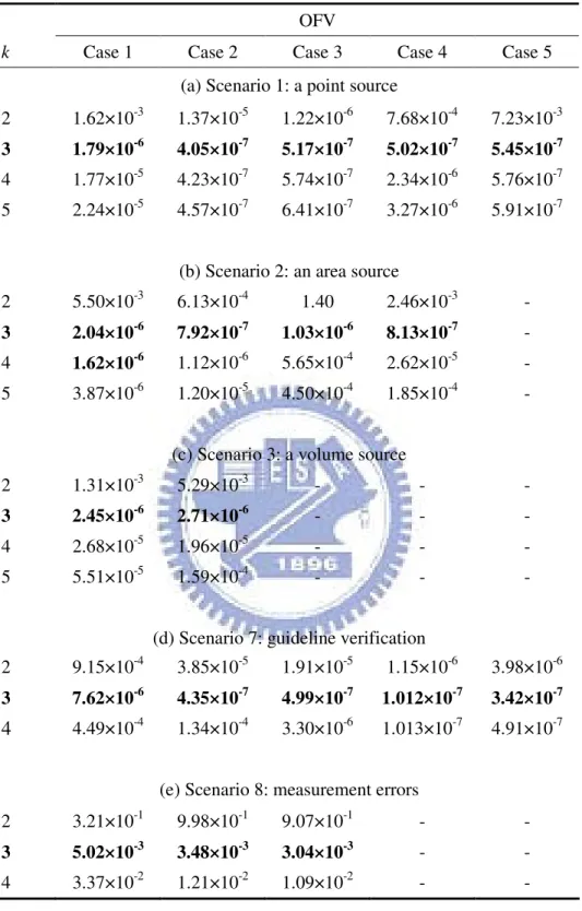
Table 1 The OFV for different k based on spatial concentration data. ...49

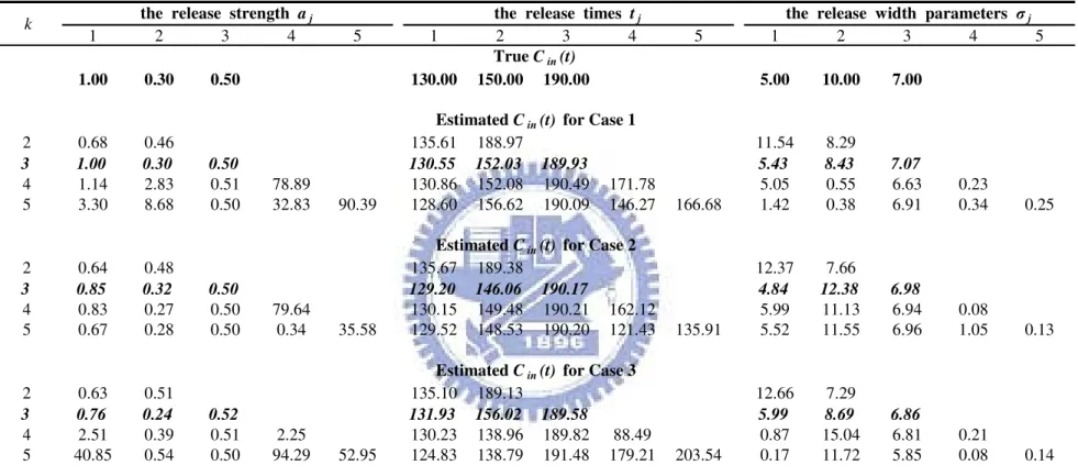
Table 2 Scenario 1: estimated parameters in the assumed release function for different k. ...50

Table 3 Scenario 2: estimated parameters in the assumed release function for different k. ...52

Table 4 Scenario 3: estimated parameters in the assumed release function for different k. ...53

Table 5 The OFV for different k based on temporal concentration data. ...54

Table 6 Scenario 4: estimated parameters in the assumed release function for different k. ...55

Table 7 Scenario 5: the best possible parameters of source release function. ...56

Table 8 Scenario 6: the sampling concentration data for cases 1 – 7...57

LIST OF FIGURES

Fig. 1. Scenario 1: sampling data at 225 days...59

Fig. 2. Scenario 1: the recovered source release histories for cases 1 - 5. ...60

Fig. 3. Scenario 1: the recovered source release history when k = 4 for cases 2, 3, and 5. ...61

Fig. 4. Scenario 2: Sampling data at 225 days. ...62

Fig. 5. Scenario 2: the recovered source release history when k = 4 for case 1...62

Fig. 6. Scenario 2: the recovered source release histories for cases 1 - 4. ...63

Fig. 7. Scenario 3: sampling concentration at 225 days. ...64

Fig. 8. Scenario 3: the recovered source release histories for cases 1 – 4...64

Fig. 9 Scenario 4: (a) case 1, 4 wells with 16data; (b) case 2, 3 wells with 15data; (c) case 3, 2 wells with 16data; and (d) case 4, 1well with 15data...65

Fig. 10. Scenario 4: the recovered source release history when k = 4 and 5 for case 1...66

Fig. 11. Scenario 4: the recovered source release histories for cases 1 - 4...67

Fig. 12. Scenario 5: different number of sampling data at (40, 0) for cases 1 - 7. 68 Fig. 13. Case 8 in scenario 6: (a) data sampled at (40, 0) from 147 to 249 days; (b) the recovered source release history. ...69

Fig. 14. Case 9 in scenario 6: (a) data sampled at (40, 0) from 153 to 230 days; (b) the recovered source release history. ...70

Fig. 15. Case 10 in scenario 6: (a) data sampled at (40, 0) from 148 to 225 days; (b) the recovered source release history. ...71

Fig. 16. Case 11 in scenario 6: (a) data sampled at (200, 0) from 180 to 620 days; (b) the recovered source release history. ...72

Fig. 17. Scenario 7: nine sampling data sampled within the region of 95 % of contaminant mass. ...73

Fig. 18 Scenario 7: the recovered source release histories for cases 1 - 5. ...74

Fig. 19 Scenario 8: erroneously sampling data at T = 225 days. Case 1, ε = 0.01; case 2, ε = 0.05; case 3, ε = 0.1. ...75

Fig. 20. Scenario 8: the recovered source release histories for cases 1 - 3. ...75

Fig. 21. Scenario 9: the sampling data at MWs 1 and 2 for cases 1 - 3. ...76

Fig. 22. Scenario 9: the recovered release histories of (a) source 1 and (b) source 2, for cases 1 - 3. ...76

NOTATION

ai A coefficient defined by Eq.(18) aj The release strength of the plume B Width of the aquifer [L]

B1 Beginning coordinate of the source in the y-direction B2 Ending coordinate of the source in the y-direction

C Concentration

∂C/∂t The change in solute concentration with time [ML-3T-1]

C(x, y, z, t) The contaminant concentration in the groundwater [ML-3]

Cext(xn,T) The exact concentration at location xn at time T Cmeas(xn,T) The measured concentration at location xn at time T Cin Contaminant source release function [ML-3]

Cini The ith contaminant source release function

CTi,est The concentration estimated at ith measurement point at time T CTi,obs The concentration measured at ith measurement point at time T D The hydraulic dispersion coefficient tensor [L2T-1]

Dx x-component of the dispersion tensor Dy y-component of the dispersion tensor Dz z-component of the dispersion tensor

E The system energy

F A kernel function defined by Eq.(7)

H Depth of the aquifer [L]

H1 Beginning coordinate of the source in the z-direction H2 Ending coordinate of the source in the z-direction k The number of the terms needed in exponential function

kB Boltzmann constant of nature which relates temperature to energy Kd Chemical degradation rate [T-1]

Ke* Modified heat exchange coefficient

L1 Beginning coordinate of the source in the x-direction L2 Ending coordinate of the source in the x-direction MAXEVL Maximum number of iteration to terminate the algorithm

min f The objective function defined by Eq.(23)

NS The number of cycles

NT The number of iterations before temperature reduction OFV

P(E)

Objective function value

Probability defined by Eq.(19) and (20)

Rd RT

Retardation factor

A cooling temperature factor

t Time

tevol The plume evolution times tj The release times of the plume

T Sampling time

Temp Temperature

Tinitial Initial temperature

v Average linear velocity vector [LT-1]

x Longitudinal coordinate

xi The x coordinates of the ith plume source xn The location of the nth sample

xs x-coordinate of a point source Xi Either function X1 or X2 X1 A function defined by Eq.(8) X2 A function defined by Eq.(9)

y Transfer coordinate

yi The y coordinates of the ith plume source ys y-coordinate of a point source

Yj Either function Y1, Y2, Y3, or Y4 Y1 A function defined by Eq.(10) Y2 A function defined by Eq.(11) Y3 A function defined by Eq.(12) Y4 A function defined by Eq.(13)

z Vertical coordinate

zs z-coordinate of a point source Zk Either function Z1 or Z2 Z1 A function defined by Eq.(14) Z2 A function defined by Eq.(15)

δn The random number from a Gaussian standard population

▽ Gradient operator

λ Radioactive decay constant

τ Time

ki i-th eigenvalue defined by Eq.(17)

ψi i-th eigenfunction defined by Eq.(16)

σ One standard deviation of the contaminant distribution σj The release width parameters of plume

CHAPTER 1 INTRODUCTION

1.1.

Background

Recently, many soil and groundwater contamination events have been reported in

Taiwan. These reports reveal that people’s health may be impaired if living near the

contaminated sites. Therefore, an effort should be made to investigate the

contaminant source and assess the remedial measures. Generally speaking,

groundwater contaminants may originate from the disposal of wastewater for various

purposes. All sources and causes of contamination can be classified into two

categories: point sources and non-point sources. Point sources, characterized by the

presence of identifiable sources, include storage tanks, pipeline releases, and chemical

manufacturing locations. Non-point sources are referred to as larger-scale and more

diffuse contamination originated from many smaller sources; for example, the

agricultural fertilizers leaching through soil and finally affecting aquifers (Todd and

Mays, 2005).

Taiwan EPA promulgated the Soil and Groundwater Remediation Act in 2000 to

require the remediation for groundwater contamination if the concentration exceeds

regulation standard. However, the remediation of groundwater contamination may

be expensive, and the responsible party rather than the public should pay the costs.

mass before groundwater remediation. This information could be estimated while

the source release history, including the release concentration and release time, is

reconstructed. Therefore, recovering source release history can provide forensic

information to determine the liability among the responsible parties.

1.2.

Literature Review

Recovering the source release history of a plume is an ill-posed problem since

contaminant transport in groundwater is a dispersive and irreversible process. In the

past two decades, many researchers have investigated this problem. Atmadja and

Bagtzoglou (2001) reviewed the methods that had been developed during the past 15

years to identify the contaminant source location and recover the time-release history.

They classified the contaminant transport inversion methods into four categories.

They are: (1) optimization approaches, (2) probabilistic and geo-statistical simulation

approaches, (3) analytical solution and regression approaches, and (4) direct

approaches.

Optimization approaches, the early methods to identify the pollution source by

solving the advection-dispersion equation (ADE), are to run forward simulations first

and check the solutions with the spatial observed data. Wanger (1992) combined

groundwater flow and contaminant transport simulation with non-linear maximum

parameters and source characteristics based on observations of hydraulic head and

contaminant concentration. He pointed out that the source could be characterized by

a set of unknown parameters.

Probabilistic and geo-statistical simulation approaches are to identify the source

release history of a plume relying on probabilistic framework. In these approaches,

the recovered release history is considered as a random process, defined through its

probability density function and its statistical moments, so it can be determined with

uncertainty. Butera and Tanda (2003) adopted the geo-statistical approach to model

the ADE backward in time. Their applications focus on the incorporation of an area

and two point sources in two-dimensional groundwater flow system with infinite

domain. Boano et al. (2005) also applied the geo-statistical method to identify the

contaminant sources in river pollution problems. Similar to Butera and Tanda (2003),

they considered an area source and two point sources. Woodbury et al. (1998) used

the minimum relative entropy inversion (MRE) to reconstruct a three-dimension

plume source. They explained how MRE inversion can be used as a measure of

resolution in linear inversion, and indicated the temporal concentration data at a few

wells can be used to reconstruct the release history of a groundwater contaminant.

Much effort has been directed to the theoretical and mathematical problems of

techniques to estimate the residual DNAPL mass. They used a tractable analytical

approximation to the problem and developed additional simplifications to yield a form

that can be solved for the parameters of interest. Alapati and Kabala (2000) applied

the nonlinear least-squares (NLS) method to recover the gradual and the catastrophic

release scenarios from its spatial concentration data. They found that the NLS

method could resolve the catastrophic release histories well, even in the presence of

moderate measurement errors.

Direct approaches use deterministic methods to solve the governing equations

reversely. Skaggs and Kabala (1994) used Tikhonov regularization (TR) to recover

the release history of a plume. TR was used to obtain a best possible solution of a

one-dimensional solute transport through a homogeneous medium with a complex

contaminant release history. Skaggs and Kabala (1995) used the quasi-reversibility (QR) method for the same problem solved in TR method. In QR method, a moving

coordinate system was used to account for the velocity term of the ADE. Skaggs and

Kabala (1998) extended their study of TR and employed Monte Carlo approach to

infer the ability of recovering an arbitrary plume in a transport medium with

dispersive characteristics.

Although previous literatures provide various methods to solve the source release

geometries, e. g., point source or area source; in addition, they all utilize more than 36

sampling concentrations to recover the source release history of a groundwater

contaminant.

1.3.

Objectives

The objective of this thesis is to design a novel method capable of solving the

source release history recovery problem in an easy and effective way and to

demonstrate that the proposed method is applicable to point source and non-point

source cases as well. The method combines a function-fitting technique and

simulated annealing (SA) with a fundamental solution of ADE. The solution of ADE

describes the contaminant released from a source into a homogeneous aquifer.

Therefore, the sampling concentrations in the stage of model development can be

created from the fundamental solution at a known location with a “true” release

function. For source release history recovery problem, the release history at a

specific source location is unknown and can be estimated by a function-fitting

technique. The source release history is assumed as a combination of several

exponential functions, and SA based on trial and error assessment generates the values

of parameters in the assumed release function. The simulated concentrations are

then calculated by the fundamental solution with the trial source release function.

concentrations, SA can determine the optimal parameters of the assumed release

function. Finally, the curve of source release history could be easily observed after

plotting the determined function.

Various field cases of the contaminant transport in one-, two-, and three-

dimensions are considered and analyzed by the proposed approach. In addition,

three types of contaminant source geometries and two different aquifer configurations

are evaluated. The source geometries include point, area, and volume sources. The

aquifer configurations contain both infinite width and finite width aquifers. Besides,

both spatial and temporal concentration data are used to analyze the influences of

contaminant biodegradation, the location of monitoring well, the degree of dispersion,

measurement errors, and the number of sampling data on the results of reconstruction.

An aquifer system may be polluted by several different contaminant sources at known

spots; therefore, whether the method could distinguish the contamination proportions

between two adjacent sources is investigated, too. Finally, a general guideline

regarding to the sampling period and sampling region in recovering the source release

CHAPTER 2 METHODS

2.1

Advection-Dispersion Equation

Advection and hydrodynamic dispersion are the main mechanisms that make the

dissolved contaminant spread and migrate in groundwater. Advection, the most

significant mass transport process that the contaminant carried by the flowing

groundwater, results from the gradient in fluid head. Hydrodynamic dispersion, a

microscopic phenomenon, is caused by a combination of mechanical dispersion and

molecular diffusion. Mechanical dispersion causes contaminant to spread out, owing

to the variation of flow path and velocity in the groundwater movement. Molecular

diffusion is the process in which the contaminants move from high concentration area

to low concentration area due to concentration gradient.

For a steady uniform flow, the ADE for contaminant transport in saturated,

homogeneous and isotropic porous media may be written as (Yeh, 1981):

(

)

( )

C R K vC C D t C d d       + − ∇ − ∇ ⋅ ∇ = ∂ ∂ λ (1)

where ∂C/∂t is the change in solute concentration with time [ML-3T-1], ▽ is gradient

operator, D is the hydraulic dispersion coefficient tensor [L2T-1], v is the average

linear velocity in x- direction [LT-1], Kd is the degradation rate [T-1], λ is the

For source release history recovery problem, the source location is known. The

source release history of a groundwater contaminant could be identified by solving

Eq.

(1) with reversed time subject to following initial and boundary conditions:

(

x,y,z,0

)

=0 C (2)

(

x ,y ,z ,t

)

C (t) C _{s s s} = _in (3)

(

±∞,y,z,t

)

=0 C (4)

(

x,±∞,z,t

)

=0 C (5)

where xs, ys, and zs are the x, y, and z coordinates of the plume source, respectively,

and Cin(t) is the contaminant source release function.

Contaminant transport is a dispersive and irreversible process; as a result,

modeling groundwater contaminant transport with reversed time is an ill-posed

problem whose solution does not satisfy general condition of uniqueness or stability.

Accordingly, the strategy of the proposed method is to avoid solving the ill-posed

problem directly. Instead, a relative well-posed problem is formulated and solved.

2.2

Analytical Modeling

The relative well-posed problem relies on a framework of an analytical model.

Analytical model is one of useful and convenient tools for analyzing and predicting

groundwater contaminant transport for a field contamination problem. Therefore, an

by Yeh (1981) is used to simulate the spatial-temporal concentration distribution of

contaminant in a groundwater flow system. Assume that the aquifer is homogeneous

and isotropic, the flow is steady and uniform, and the source release is continuous.

The solution for Eq. (1) subject to initial and boundary conditions of Eqs. (2) - (5) can

be written as:

∫

− = T in F x y z T d C t z y x C 0 ) , , , ( ) ( ) , , , ( τ τ τ (6)

where T is the sampling time, C(x, y, z, T) is the plume concentration in the

groundwater [ML-3], and F(x, y, z, T-τ) is the fundamental solution of ADE, or called

kernel function. Notice that the function F(x, y, z, T-τ) is chosen dependent on the

source geometry and aquifer configuration. In AT123D, F(x, y, z, T-τ) for

three-dimensional case is expressed as:

(

x y z T

)

XiYjZk

F , , , −τ = (7)

where X, Y, and Z denote the source in x, y, and z direction, respectively, and the

subscripts i, j, and k signify the type of source geometries and aquifer configurations.

The AT123D contains various options and these options are the combination of

different type of contaminants, source geometries, source release, and aquifer

configurations. In this study, three types of source geometries and two kinds of

aquifer configurations are considered. The source geometries are point, area, and

the functions Xi, Yj, and Zk, chosen fromAT123D, are given as follows:

for point source in the x-direction:

(

)

(

)

{

}

(

)

(

)

_      −       + − − − − − − − = λ τ τ τ τ π R T K T D T v x x T D X d d x s x 4 exp ) ( 4 1 2 1 (8)

for line source in x-direction:

(

)

(

)

(

)

      −       + − ⋅                 − − − − −         − − − − = λ τ τ τ τ τ T R K T D T v L x erf T D T v L x erf X d d x x exp ) ( 4 ) ( 4 2 1 _{1 2} 2 (9)

for finite width and point source in the y-direction:

(

)

∑

∞ =         −       − ⋅       ⋅       + = 1 2

1 cos cos exp

2 1 i y s T D B i B y i B y i B B Y π π π τ (10)

for finite width and line source in the y-direction:

(

)

        −       −             −       ⋅       + − =

∑

∞ = τ π π π π π T D B i B B i B B i i B B y i B B B B Y y i 2 1 1 2 1 2 2 exp sin sin cos 2 (11)

for infinite width and point source in the y-direction:

(

)

(

)

(

)

_      − − − − = τ τ π D T y y T D Y y s y 4 exp 4 1 2 3 (12)

for infinite width and line source in the y-direction:

(

)

(

)

_                − − −         − − = τ τ D T B y erf T D B y erf Y y y 4 4 2 1 _{1 2} 4 (13)

for finite depth and point source in the z-direction:

( ) ( )

[

(

)

]

∑

∞ = + − − ⋅ = 1 2 1 1 exp i z i s i i H T D k z z Z ψ ψ τ (14)

for finite depth and line source in the z-direction:

( )

(

)

(

)

∑

∞ = − −       + − = 1 1 2 1 2 2 {sin sin i i i i i i kH kH k a z H H H Z ψ

(

)

(

)

[

−

]

⋅

[

−

(

−τ

)

]

∗ T D k H k H k k D K z i i i i z e 2 1 2 cos } exp cos (15)

where B and H are respectively the width and the depth of the aquifer [L]; L1, B1, H1

and L2, B2, H2 are respectively the beginning and the end coordinates (x, y, z) of the

source [L]; Dx, Dy and Dzare respectively the component of the dispersion tensor in x-,

y-, and z- directions [L2T-1]; K_e∗ is the modified heat exchange coefficient. In Eqs.

(14) and (15), ψi(z) is:

( )

( )

( )

      + = ∗ z k k D K z k a z _i i z e i i i cos sin ψ (16)

where ki and ai are given as:

(

)

i z e i k D K H k ∗ = tan (17) and

(

) (

)

{

e z i e z i

}

i X D K k D K H a ∗ ∗ ₊ + = ₂ 2 1 2 (18)

The selection of fundamental function depends on the source geometry and

aquifer condition. Once F(x, y, z, T-τ) is selected, the distribution of a groundwater

plume concentration can be simulated by applying the Gaussian quadrature to

2.3

Optimization by SA

The following part will introduce how SA could determine the parameters of the

assumed function in detail. SA is a heuristic search method, and the algorithm of SA

is in analogy to thermodynamics of liquids freezing and crystallizing. If a hot liquid

is cooled slowly, a pure crystal can be formed. This crystal is in the state of

minimum energy for the system. However, if the liquid is cooled quickly, the pure

crystal may not be formed, and the system may then be in the state of a local

minimum energy. The energy probabilistic distribution of a system is expressed by

Boltzmann probability distribution as:

(

)

(

E kBTemp

)

E

P( )∝ exp − (19)

where the P(E) is probability, E is the system energy, kB is Boltzmann constant of

nature which relates temperature to energy, and Temp is the temperature. According

to Eq. (19), the system has chance to run away from a local minimum energy to more

global one, since lower probability may be occurred with high energy state at low

temperature of a system ( Press et al.,1986).

A modified Boltzmann probability function named as the Metropolis’ criteria

(Kirpatrick, 1983) is adopted in SA. The Metropolis’ criteria supply a more efficient

simulation of thermal motion of atoms in equilibrium of a given temperature. In

thermodynamics system is to change its configuration from energy E1 to energy E2.

∆E = E2 - E1. If ∆E ≤ 0, the displacement is accepted, and the displaced atom is used

as the starting point of the next step. The case ∆E > 0 is treated probabilistically.

The Metropolis’ criteria are written as follows (Pham and Karaboga, 2000):

(

)

(

)

     >        _{− −} ≤ = ∆ 1 2 1 2 1 2 , exp , 1 E E if T k E E E E if E P emp B (20)

If E2 > E1, one has to check the Metropolis’ criteria. A random number uniformly

distributed in interval (0, 1) is selected and compared with P(∆E). If the random

number is smaller than P(∆E), then the displaced atom replaces the original one.

Otherwise, the original atom is used to start the next step.

The procedure of SA is an iterative improvement, and the Metropolis’ criteria

provide a general inference of iterative improvement. To implement SA, an initial

guess of the solution, called current optimal solution, is set to calculate the current

objective function in analog of energy. Then, NS random trial solutions are created

and the objective function values (OFV) of the trial solutions are computed by SA.

Once the OFV of the trial solutions satisfies the Metropolis criteria, the trial solution

is accepted and replaces the current optimal solution. Otherwise, the trial solution is

rejected. After NT times through the loops, the temperature, Te, is reduced. As the

the optimal solution or the system satisfies the terminal temperature or iteration

CHAPTER 3 HISTORY RECOVERY PROCESS

In this chapter we illustrate the two-step process of the proposed method to

recover the source release history of a groundwater contaminant. The first step is to

create the sampling concentrations at the monitoring wells. A numerical example

given in Skaggs and Kabala (1994) is employed to generate the sampling

concentrations. The “true” source release function with a three sinuous waves for a

non-reactive contaminant source given by Skaggs and Kabala (1994) was:

(

)

(

)

(

)

        ₋ − +         ₋ − +         ₋ − = ₂ 2 2 2 2 2 ) 7 ( 2 190 exp 5 . 0 ) 10 ( 2 150 exp 3 . 0 ) 5 ( 2 130 exp ) (t t t t C_in (21)

where 130, 150, and 190 are the source release times; 5, 10, and 7 are a measure of

the spread of the release function; 1, 0.3, and 0.5 are the release strength of source.

The fundamental solution, F(x, y, z, T-τ), is chosen based on the source geometry and

aquifer configuration. The distribution of plume concentration can be created based

on Eqs. (6) and (21) with given aquifer parameters; thus, the sampling concentration

data are acquired.

The second step is to apply the function-fitting technique to solve the source

release history recovery problem. Lin (1999) mentioned that any continuous

function on a closed and bounded interval can be approximated on that interval by

sampling data and produce a smooth curve, then it can be considered as a proper

model. Accordingly, a source release function may be expressed as (Alapati and

Kabala, 2000):

(

)

∑

=        _{− −} = k j j j j in t t a t C 1 2 2 2 exp ) ( σ (22)

where k is the number of the terms needed in exponential function, aj is the release

strength of the source, tj is the release times of the source, and σj is the release width

parameters of source. The value of k represents the number of source release waves;

thus, k = 3 in Eq. (21).

The SA is applied to produce the trial values for parameters in Eq. (22), i.e., aj, tj,

and σj. The simulated concentrations are then generated from Eqs. (6) and (22) with

those trial parameters. The optimal parameter values can be determined as the

objective function is minimized. The objective function in SA is expressed as

(

)

∑

= − = n i T sam i T sim i C C f 1 2 , , min (23)

where CTi,sim is the simulated concentration estimated at ith monitoring well at

sampling time T, CTi,sam is the sampling concentration measured at ith monitoring well

at sampling time T, and n is the number of monitoring wells.

In SA, an initial guess of the parameters in the assumed function is set to

calculate the simulated concentrations based on Eqs. (6) and (22), then the initial OFV

their OFV of the trial solutions. If the OFV of the trial solution is smaller than that

of the current value, the trial solution is taken as the current optimal solution. If not,

Metropolis’ criteria are applied to accept or reject the poorer solution. The

temperature is reduced after NT times through the above loops. The algorithm will

be continued until SA obtains the optimal solution or the system satisfies the terminal

temperature or iteration numbers.

The variable k in Eq. (22), representing the wave numbers in the source release

function, is a crucial problem to solve. The value of k can be determined by

selecting the one which has the least value of the OFV, or can be chosen directly

based on the shape of the concentration distribution which to some extent reflects the

pattern of the source release history

To employ SA, the number of trial solution for each unknown (NS) and the

annealing schedule must be defined. The annealing schedule consists of the initial

temperature (Tinitial), a cooling temperature factor (RT), the iteration number before

decreasing the temperature (NT), and maximum number of iteration to terminate the

algorithm (MAXEVL). No general rule is applicable in choosing these parameters.

In this study, Tinitial, NS, NT, RT, and MAXEVL are given as 100, 30, 5, 0.8, and 106

by trial-and error approach. Poor guesses will give spikes in the recovered release

CHAPTER 4 SCENARIOS AND RESULTS

Nine scenarios are designed to demonstrate the proposed method in solving the

source release history recovery problem. Scenarios 1 – 3 are intended to show that

the proposed method is applied to the case of one-dimensional point source and then

to the case of two- and three-dimensional non-point sources. In addition, two

different aquifer configurations are considered for two- and three-dimensional

groundwater transport; one is that the aquifer has infinite width while the other

considers the width of the aquifer is finite. Scenario 1 attempts to recover a point

source release history for contaminant in one-, two-, and three- dimensional transports.

Scenario 2 aims to reconstruct an area source release history for contaminant in two-,

and three-dimensional transports. Scenario 3 aspires to recover a volume source

release history for contaminant in three-dimensional transport. The effect of

contaminant biodegradation on the result of reconstruction is also investigated in

scenario 3. These three scenarios employ spatial concentration data sampled from

17 monitoring wells.

Scenario 4 is used to investigate whether the temporal concentration data

sampled at few wells could recover the source release history or not because more

spatial concentration data implying higher cost involved in installing monitoring wells.

explore the required numbers of temporal concentration data for solving the source

history recovery problem. In scenario 6, temporal concentration data are utilized to

establish a general guideline on the sampling period and sampling region in

recovering the source release history.

Scenario 7 intends to prove that the guideline drawn from scenario 6 is also

applicable to analyze the spatial concentration data. In scenario 8, normally

distributed noise is added to the sampling concentrations to investigate the capability

of the proposed method in recovering the source release history. An aquifer system

may be polluted by several sources at different times from known locations.

Therefore, scenario 9 is to test whether the proposed method can handle the composite

contamination form two adjacent sources or not. The influences of the location of

monitoring wells and the degree of dispersion on the result of recovering release

history are also explored in scenario 9.

Since this study is based on the analytical approach to recover the source history,

each scenario assumes that the aquifer is homogeneous and isotropic; the flow is

steady and uniform; the contaminant is conservative, no decay, and no adsorbed on

the aquifer. Various aquifer parameters and the source geometry and location are

4.1 Scenario 1: Point Source

Scenario 1 attempts to recover a point source release history for contaminant in

one-, two-, and three- dimensional transports. Five cases are designed to assess the

applicability of the proposed approach. Assume the point source is located at the

origin, i.e., (xs, ys, zs) = (0, 0, 0), and the aquifer is clean and the background

concentration is zero at the beginning. Suppose the aquifer is infinite in x-direction

and finite in z-direction (0 < z < 3 m). Two types of aquifer configurations are

considered; one has an infinite width while the other has a finite width in y-direction.

In case 1, a one-dimensional plume in the x-direction with the kernel function, F,

equaling X1 in Eq. (8) is considered. In case 2, a two-dimensional transport in the

x-y plane with F = X1 Y3 in Eqs. (8) and (12) is studied. In case 3, a

three-dimensional plume with F = X1 Y3 Z1 in Eqs. (8), (12), and (14) is investigated.

For cases 2 and 3, the aquifer is infinite in y-direction while for cases 4 and 5, the

aquifer has a finite width of 100 m. Case 4 supposes the plume is two-dimensional

and distributed in the x-y plane with F = X1 Y1in Eqs. (8) and (10). Case 5 assumes

to have a three-dimensional plume with F = X1 Y1 Z1 in Eqs. (8), (10), and (14).

With Eqs. (6) and (21), the plume concentration is estimated by using the

parameters v, Dx, Dy, and Dz being equal to 1 m/day, 1 m2/day, 0.1 m2/day, and 0.1

1 – 5, revealing that the originally three distinct release waves of the source have been

released at 225 days. The monitoring wells are installed from 0 m to 160 m with a

uniform interval of 10m along x-axis. Thus, 17 spatial concentration data are

available for recovering the source release history.

A function fitting technique is applied to solve the source release history

recovery problem, and the source release history of groundwater contaminant is

represented by Eq. (22) which contains three parameters, aj, tj, and σj. Totally 3k

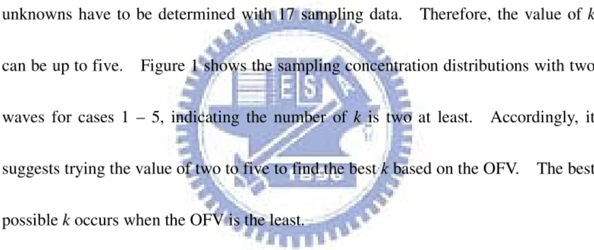
unknowns have to be determined with 17 sampling data. Therefore, the value of k

can be up to five. Figure 1 shows the sampling concentration distributions with two

waves for cases 1 – 5, indicating the number of k is two at least. Accordingly, it

suggests trying the value of two to five to find the best k based on the OFV. The best

possible k occurs when the OFV is the least.

Table 1(a) lists the OFV for different k in cases 1 – 5, indicating that the

objective function has a least value when k = 3. Table 2 shows the estimated

parameters determined by SA, also revealing that the estimated release history

function is exact when k = 3. Hence, we conclude that the release history is

recovered when the OFV is the least among different k. Figure 2 displays the

recovered release histories of the five cases when k = 3. For case 1, the

aquifer with infinite width, the release history represented by the dashed line shown

in Figs. 2(b) and 2(c) for cases 2 and 3 respectively is recovered acceptably, except

the first wave is somewhat underestimated. In contrast, the first pattern of the

reconstruction gives a little overestimation in cases 4 and 5 for aquifer with a finite

width of 100 m, as displayed in Figs. 2(b) and 2(c), respectively. Those results

confirm that the proposed approach gives good estimated results as compared with

the true one. In other words, the exponential function is suitable to use as the basis

of the release history and the SA can successfully estimate the parameters (the

release strength, release times, and release width) of the source release history as

well.

However, attention should be paid to the OFV when k = 4 in cases 2, 3, and 5,

since it is close to the OFV when k = 3. Figure 3 displays the recovered release

history when k = 4 for cases 2, 3, and 5, with one spike appeared in the reconstructed

history. In case 2, the spike occurs at 172 days while it appears at 88 and 163 days

in cases 3 and 5, respectively. In addition, the first wave in case 3 and the middle

wave in case 5 are overestimated. These results indicate that the source release

history recovered for the case with OFV, which is not the least one, can lead to a

4.2

Scenario 2: Area Source

For the real field problem, the use of point source is a simplified assumption

since the source geometry of contamination to some extent has dimension, e.g., source

discharging from irrigation practices or fertilizer applications. Therefore, scenario 2

aims to reconstruct the release history of an area source for contaminant in two- and

three-dimensional transports. Four cases are designed to analyze the application of

the proposed method while considering two aquifer configurations of finite width and

infinite width. The aquifer dimensions and the aquifer parameters are set the same

as scenario 1. The dimensions of the area source are 5m × 5m.

The sampling concentrations can be calculated based on Eqs. (6) and (21) with

appropriate kernel functions. In case 1, the two-dimensional transport in the x-y

plane with F = X2 Y4 in Eqs. (9) and (13). In case 2, the proposed method is used to

recover the release history of a three-dimensional plume with F = X2 Y4 Z1 in Eqs. (9),

(13), and (14). Consider the aquifer is infinite in the y-direction in cases 1 and 2

while it is finite with the width of 100 m in cases 3 and 4. Case 3 considers that the

plume is two-dimensional and distributed in the x-y plane with F = X2 Y2 in Eqs. (9)

and (11). Case 4 assumes to have a three-dimensional plume with F = X2 Y2 Z1 in

Eqs. (9), (11), and (14).

4, displaying 17 sampling concentrations are available to reconstruct the source

release history. Since 3k unknowns are to be determined with 17 sampling data and

the sampling concentration distributions shown in Fig. 4 imply that the number of

release waves of the source is at least two. Thus, the number of source release

waves, k, is chosen from two to five to find the suitable k which occurs when the OFV

has a least value. Table 1(b) lists the estimated OFV for different k in cases 1 – 4,

indicating that the least OFV occurs when k = 3, except case 1 in which the least OFV

occurs when k = 4.

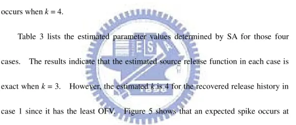
Table 3 lists the estimated parameter values determined by SA for those four

cases. The results indicate that the estimated source release function in each case is

exact when k = 3. However, the estimated k is 4 for the recovered release history in

case 1 since it has the least OFV. Figure 5 shows that an expected spike occurs at

184 days in the recovered history when k = 4 in case 1. Because a smooth curve for

the release history is a better choice in reality; thus, the recovered source release

history when k = 3 is adopted. Figure 6 displays the recovered release histories of

cases 1 – 4 when k = 3, reflecting the recovered release histories of these cases match

with the true one very well. Those results imply that the proposed approach can

reconstruct the release history from an area source. In addition, the results also

least value among different k.

4.3

Scenario 3: Volume Source

When contaminant is not originated from a point source but from a large less

well-defined space, it may be approximated by a volume source. Scenario 3 intends

to recover a volume source release history for contaminant in three-dimensional

transport. The volume source dimensions are as follows: L1 = 0 m and L2 = 5 m for

the length, B1 = 0 m and B2 = 20 m for the width, and H1 = 0 m and H2 = 2 m for the

depth. Four cases are designed to assess the performance of the proposed method.

For cases 1 and 2, two different aquifer configurations are considered, respectively.

In case 1, the aquifer is infinite in the y-direction while for case 2 it is assumed to

have a finite width of 100 m. Suppose the depth of the aquifer is 10 m and the

aquifer is infinite in x-direction. The sampling concentrations are generated with the

same aquifer parameters as used in scenario 1.

Because the kernel function is chosen based on the source geometry and aquifer

configuration, therefore, the kernel function equals X2 Y4 Z2 defined in Eqs. (9), (13),

and (15) for case 1, and X2 Y2 Z2 in Eqs. (9), (11), and (15) for case 2. With Eqs. (6)

and (21), the spatial concentration distributions for cases 1 and 2 are calculated and

shown in Fig. 7; therefore, a set of 17 sampling data is available for recovering the

for both cases is at least two.

The unknown release history of a groundwater contaminant is represented by Eq.

(22) with 3k unknowns. For 3k ≤ 17, the number of the terms, k, can be up to five.

Hence, the trial number of release waves, k, can be from two to five. Table 1(c) lists

the estimated OFV for different k in cases 1 and 2, indicating that the least OFV

occurs when k = 3. Table 4 lists the estimated parameters determined by SA and

verifies that the estimated release history function is exact when k = 3. Based on the

obtained parameters when k = 3, the curve of source release history can be shown

graphically. Figure 8 displays the recovered release histories of cases 1 and 2,

showing that the reconstructions of both cases are in good agreement with the true one,

even though the middle wave is not observed in the sampling concentration

distribution. These results demonstrate that the proposed method provides a robust

tool for recovering a volume source release history of a groundwater contaminant and

can be applied to the cases of multi-dimensional non-point source as well.

Cases 3 and 4 are designed to investigate the impact of contaminant

biodegradation on the reconstruction of case 1. Both cases consider the

biodegradation rate, λ, of 0.0055 day-1 if the contaminant is the Trichloethene and is

biodegradable under aerobic oxidation condition. We assume the λ is known in case

concentrations of those two cases which consider the contaminant biodegradation.

The recovered release histories for cases 3 and 4 are shown in Figure 8. In case 3

with the known λ, the source release history is reconstructed very well if compared

with the true one. As for case 4, the estimated λ is 0.0039374 day-1 by SA with the

upper and lower bounds of 0. and 0.0278 day-1 (Bedient et al., 1999) for λ. The

source release history is recovered acceptably since the release width of the first wave

is slightly underestimated and the release strength of the third wave is overestimated.

The result reveals that the proposed approach also can reconstruct the source release

history reasonably well if λ is unknown.

4.4

Scenario 4: Number of Monitoring Well

For spatial concentration data, a large number of monitoring wells are often

needed to accurately capture the information of the plume. It implies the relative

high cost involved in installing the monitoring wells. Therefore, for cost saving,

scenario 4 proposes to investigate whether the proposed approach can use the

temporal concentration data sampled at few wells to recover the source release history.

Four cases are designed to investigate the effect of the number of the monitoring wells

on the results of reconstruction of the source release history. A two-dimensional

plume in an infinite aquifer from a finite area source is considered. The dimensions

calculated based on the parameter set with v = 1 m/day, Dx = 0.5 m2/day, and Dy =

0.05 m2/day.

The number of monitoring wells considered in cases 1 – 4 is from 4 to 1,

respectively. In case 1, 4 wells are located at (40, 0), (60, 5), (80, 5), and (80, 10),

and there are totally 16 sampling concentrations measured from 160 to 250 days in 30

days time increments. For case 2, three monitoring wells are placed at (40, 0), (60,

5), and (80, 10), and there are 15 concentrations sampled from 150 to 270 days in 30

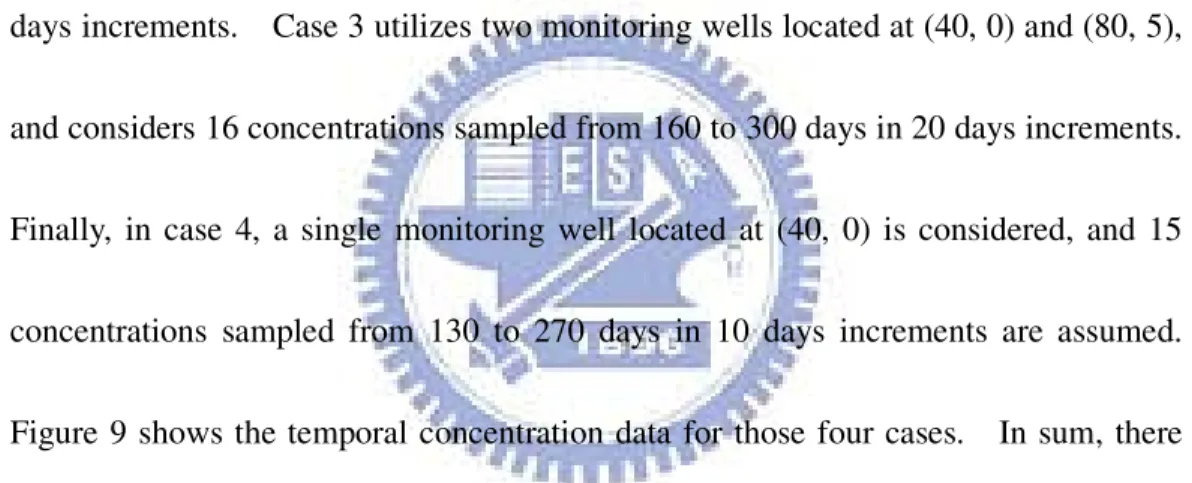
days increments. Case 3 utilizes two monitoring wells located at (40, 0) and (80, 5),

and considers 16 concentrations sampled from 160 to 300 days in 20 days increments.

Finally, in case 4, a single monitoring well located at (40, 0) is considered, and 15

concentrations sampled from 130 to 270 days in 10 days increments are assumed.

Figure 9 shows the temporal concentration data for those four cases. In sum, there

are 16 sampling data for cases 1 and 3 and 15 sampling data for cases 2 and 4 to

reconstruct the source release history.

Following the same recovery procedure as mentioned in Chapter 3, the value of k

can be up to five in those four cases. Table 5(a)lists the estimated OFV for different

k in cases 1 – 4, indicating that the objective function has a least value when k = 3,

except in case 1 which has the smallest OFV when k = 4.

indicating that the estimated parameters have good accuracy when k = 3. However,

in case 1 the OFV’s are small when k ranges 3 to 5 and have the least value when k =

4. In case 1, when k = 4 and 5 the estimated first three parameters in Eq.(22) are

close to the true ones as displayed in Table 6 and the remaining terms are near zero

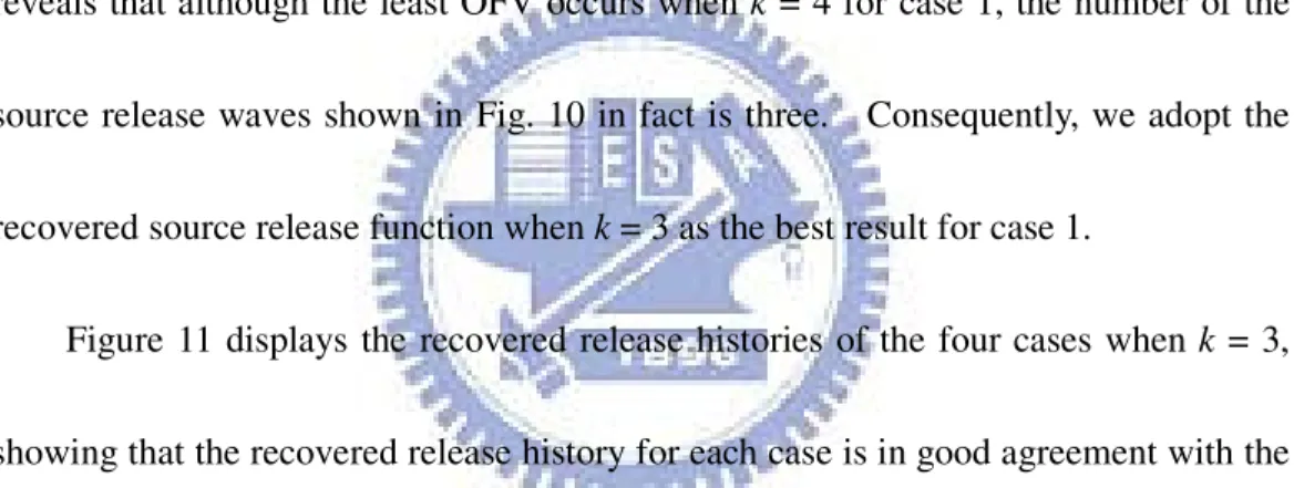
because the corresponding release width parameters are close to zero. Figure 10

shows the recovered release histories when k = 4 and 5 for case 1, displaying that the

reconstructions match with the true one, if neglecting the spike when k = 5. This

reveals that although the least OFV occurs when k = 4 for case 1, the number of the

source release waves shown in Fig. 10 in fact is three. Consequently, we adopt the

recovered source release function when k = 3 as the best result for case 1.

Figure 11 displays the recovered release histories of the four cases when k = 3,

showing that the recovered release history for each case is in good agreement with the

true one. The results demonstrate that proposed method can solve the source release

history recovery problem based on temporal concentration data for the well number

ranging from 1 – 4. In addition, the results indicate that the proposed method is

effective since only one monitoring well with 15 sampling concentration data is good

enough to solve the problem.

4.5

Scenario 5: Number of sampling data

concentration data for solving the source release history recovery problem. Seven

cases with sampling data points of 8 to 14 are designed. One monitoring well

located at (40, 0) is considered. Assume a two-dimensional plume from a finite area

source while the aquifer is infinite. The dimensions of the area source and the

aquifer parameters are set the same as scenario 4.

Figure 12 illustrates the data set of the seven cases that are analyzed. In case 1,

there are 14 sampling concentrations measured from 147 to 251 days in 8 days

increments. In case 2, totally 13 sampling concentrations are measured from 150 to

246 days in 8 days increments. Case 3 considers 12 concentrations sampled from

150 to 249 days in 9 days increments. Case 4 supposes 11 concentrations sampled

from 150 to 250 days in 10 days increments. In case 5, ten sampling concentrations

are measured from 150 to 249 days in 11 days increments. Case 6 considers nine

concentrations sampled from 150 to 246 days in 12 days increments. Finally, in case

7, totally eight sampling concentrations are measured from 150 to 248 days in 14 days

increments.

Figure 12 shows that the sampling concentration distribution with two waves for

cases 1 – 7, indicating the number of source release waves, k, is two at least. Thus,

the trial value of k can be from two to four in cases 1 – 3, from two to three in cases

case, indicating that the least OFV is obtained when k = 3 in cases 1 – 6. Notice that

the OFV for k = 3 is at least four orders less than those for k = 2 and 4 in cases 1 – 3;

and six orders less than those for k = 2 in cases 4 – 6. Hence, the best recovered

release history can be obtained when k = 3. As for case7, the source release history

could merely be reconstructed based on the estimated parameters when k = 2.

Table 7 shows the best possible parameters of the assumed release function for k

= 3 in cases 1 – 6 and for k = 2 in case 7. The result demonstrates that the estimated

parameters listed in Table 7 are in good accuracy, except in case 7. The

reconstruction in case 7 is a two-wave source release history; however, the true source

release history has a three-wave curve. Such a problem could attribute to the fact

that the number of the sampling data in case 7 is insufficient to identify the value of k.

So the required number of sampling data in this case study has to be more than or

equal to nine.

4.6

Scenario 6: A Guideline for Sampling

Based on previous studies, good reconstructions rely on the sampling

concentration data that capture adequate information of the spreading plume.

However, how do we assure that the sampled concentrations are good enough for

recovering the source release history? To answer this question, scenario 6 attempts

recovering a source release history. Eleven cases are designed to draw the guideline

on sampling region and sampling period for a two-dimensional plume in an infinite

aquifer from an area source. The aquifer parameters are set the same as scenario 4.

Seven cases are designed to investigate the effect of the monitoring well location

on the result of recovering the source release history since the monitoring well may

not locate right at the downgradient of the source. The area source dimensions are as

follows: L1 = 0 m and L2 = 5 m for the length, B1 = 0 m and B2 = 5 m for the width.

The monitoring wells in cases 1 – 7 are considered to be installed at (40, 5), (40, 6),

(40, 7), (40, 8), (40, 9), (40, 10), and (40, 11), respectively. The sampling period for

those cases ranges from 150 to 249 days with 9 days time increments. Table 8 shows

12 temporal concentrations in cases 1 – 7.

Table 5(c) lists the OFV for different k, presenting that the objective function has

a least value when k = 3 for all cases. Hence, we conclude that the best recovered

release history is obtained when k = 3. Notice that the OFV for k = 3 is at least four

orders less than those for k = 2 and 4 in case 1, revealing that a higher plume

concentration level at the monitoring well tends to give a more obvious difference in

OFV for different k. On the other hand, as the monitoring well deviates from the

center line of the plume (y = 2.5 m) more than 8 m (case 7), the difference in OFV for

Table 9 presents the parameters of the assumed release function for cases 1 – 7

when k = 3, indicating the source release histories of cases 1 – 6 are correctly

recovered; while the reconstruction of case 7, with the monitoring well located more

than 8 m from the center line of the plume in y-direction, is inaccurate. In case 7, the

three waves are out of shape since the estimated source release time has moderate

shift. The results indicate that sampling concentrations measured within 8 m from

the center line of the plume can be used to recover a source release history.

Due to plume concentrations can be described by Gaussian distribution in 1-D,

2-D, or 3-D geometries, and the spread of the plume can be determined based on the

dispersion coefficients, σ2 =2Dt_evol, where tevol is the plume evolution time (Bedient

et al., 2003). Hence, one standard deviation of the contaminant distribution in

y-direction in this case study, σ_y = 2D_yt_evol , ranges from 4.1 to 4.8 m.

Accordingly, the position of 8 m deviated from the center line of the plume in

y-direction is about 1.96σy. Therefore, the proper sampling region is suggested to be

within the area covered by ± 1.96σy from the center of the plume.

Cases 8 – 10 are designed to investigate the impact of sampling period on the

reconstruction of the source release history. The monitoring well is located at (40, 0).

There are 12 sampling data are used. In case 8, the sampling period is between 147